Analysis of horizontal zigzag manoeuvring trials from the MUN Explorer AUV

Publisher’s version / Version de l'éditeur:

Vous avez des questions? Nous pouvons vous aider. Pour communiquer directement avec un auteur, consultez la première page de la revue dans laquelle son article a été publié afin de trouver ses coordonnées. Si vous n’arrivez pas à les repérer, communiquez avec nous à PublicationsArchive-ArchivesPublications@nrc-cnrc.gc.ca.

Questions? Contact the NRC Publications Archive team at

PublicationsArchive-ArchivesPublications@nrc-cnrc.gc.ca. If you wish to email the authors directly, please see the first page of the publication for their contact information.

https://publications-cnrc.canada.ca/fra/droits

L’accès à ce site Web et l’utilisation de son contenu sont assujettis aux conditions présentées dans le site LISEZ CES CONDITIONS ATTENTIVEMENT AVANT D’UTILISER CE SITE WEB.

Oceans '08 [Proceedings], 2008

READ THESE TERMS AND CONDITIONS CAREFULLY BEFORE USING THIS WEBSITE. https://nrc-publications.canada.ca/eng/copyright

NRC Publications Archive Record / Notice des Archives des publications du CNRC :

https://nrc-publications.canada.ca/eng/view/object/?id=ca5ba12b-504a-4613-bb43-1ffb13ded587

https://publications-cnrc.canada.ca/fra/voir/objet/?id=ca5ba12b-504a-4613-bb43-1ffb13ded587

NRC Publications Archive

Archives des publications du CNRC

This publication could be one of several versions: author’s original, accepted manuscript or the publisher’s version. / La version de cette publication peut être l’une des suivantes : la version prépublication de l’auteur, la version acceptée du manuscrit ou la version de l’éditeur.

Access and use of this website and the material on it are subject to the Terms and Conditions set forth at

Analysis of horizontal zigzag manoeuvring trials from the MUN Explorer

AUV

Analysis of Horizontal Zigzag Manoeuvring Trials

from the MUN Explorer AUV

Manoj T. Issac

, Sara Adams

, Neil Bose

,

Christopher D. Williams

, Ralf Bachmayer

Tristan Crees

1

Ph.D. Student, Memorial University of Newfoundland (MUN) St. John's, NL, A1B 3X5, Canada.

Manoj.Issac@nrc-cnrc.gc.ca / M.Issac@gmail.com Ph: 001-709-7726127 (Off)/001-709-3513016 (Res)

2

Research Lab Coordinator, MERLIN, Memorial University of Newfoundland (MUN) St. John's, NL, A1B 3X5, Canada

3

Professor of Maritime Hydrodynamics and Manager, Australian Maritime Hydrodynamics Research Centre, University of Tasmania, Launceston, Tasmania 7250, Australia

(Formerly Professor, Canada Research Chair in Offshore and Underwater Vehicles Memorial University of Newfoundland)

4

Research Engineer, National Research Council Canada, Institute for Ocean Technology St. John’s, NL, A1B 3T5, Canada

5

Associate Professor, Chair for Ocean Technology, Faculty of Engineering and Applied Science, Memorial University of Newfoundland, St. John's, NL, A1B 3X5, Canada

6

Robotics Engineer, International Submarine Engineering Ltd, 1734 Broadway Street Port Coquitlam, BC, V3C 2M8, Canada

Abstract- A series of full-scale zigzag manoeuvring trials were

performed using a streamlined Autonomous Underwater Vehicle (AUV) – the MUN Explorer AUV during the summer of 2006. This paper presents the results and observations from the zigzag manoeuvres or the Z-tests performed in horizontal planes. Unlike the conventional method of performing a Z-test, these zigzags were performed by allowing the vehicle to follow a predefined path that was laid out in a zigzag pattern. The paper outlines briefly the method by which these tests were conducted and discusses the observations made.

I. INTRODUCTION

Manoeuvring trials are often performed to assess the path keeping and path changing ability of a marine vehicle. The path keeping and path changing ability of a marine vehicle are interdependent, as the practical problem of path keeping involves instances of path correction and hence the elements involved in one affects the other as well. Traditionally, naval architects have devised certain definitive manoeuvres to address these issues pertaining to path keeping and path changing. These manoeuvres such as turning circles, zigzags, spirals etc., establish the basic stability and control characteristics of a marine vehicle [1].

The purpose of performing these open water manoeuvring trials, reported in this paper, were to obtain a set of full-scale experimental data for the validation of an hydrodynamic motion simulation model developed for a streamlined

torpedo-shaped underwater vehicle. This model developed was based on the “body build-up” method of Nahon [2] which was subsequently modified by Perrault [3] and Evans [4] using MATLAB™ and SIMULINK™. The attraction of this model was its simplicity with which the hydrodynamic loads acting on vehicle were calculated by summing up the contributions from individual components. This model, while it was available for use at the Memorial University of Newfoundland, had never been validated against experimental data from real vehicle. Thus it was necessary to have some experimental data from a real vehicle. The availability of the MUN Explorer AUV at Memorial University facilitated this requirement.

MUN Explorer is a survey-class AUV built by International Submarine Engineering (ISE) Ltd., in Port Coquitlam, British Columbia. The AUV is 4.5 m in length with a maximum mid-body diameter of 0.69 m. The parallel mid-mid-body section has a semi-ellipsoidal nose at its front end and a faired tail section at its aft end which gives it a hydrodynamically efficient streamlined shape. The vehicle has a dry weight of 630 kg and is rated for 3000 m depth. It can achieve a maximum cruising speed of 2.5 m/s using a twin bladed propeller. Manoeuvring in 3-D space is facilitated by six control planes – two dive planes for precise depth control and four tail planes to control roll, pitch and yaw motions of the vehicle. The AUV essentially functions as a sensor platform for undersea survey and data collection purposes. Figure 1 shows the MUN

Explorer AUV being deployed for a mission. A detailed description of the vehicle and its various features, the equipment, the sensors and other instruments it uses can be found in reference [5]. Note the presence of large forward dive planes and the X-configuration of the four tail planes.

A series of manoeuvring trials were performed using the

A series of manoeuvring trials, which included straight-line tests, turning circles, horizontal and vertical zigzags, were performed using the MUN Explorer AUV. These tests were conducted at Holyrood Harbour, which is situated 45 km southwest of St. John’s, Newfoundland (Lat = 47.39 N and Long = 56.13 W), during the summer of 2006. This sheltered body of water had sufficient depth and spread so as to carry out all the intended tests. The water depth ranged from 10 m to 50 m and more. A detailed description of the different tests that were conducted as well as the methods and measures used to perform these were reported in detail in [5]. Further, the data analysis and observations from straight-line tests and a portion of the turning circles were reported in [6]. This paper deals with the analysis and observations from the horizontal zigzag manoeuvring trials. The next section gives a brief introduction of how the tests were performed followed by some results and observations in the subsequent section.

II. TEST PROCEDURE

A zigzag manoeuvre is indicative of the control characteristics of the vehicle. It also show the effectiveness of the rudder in controlling the vehicle. Traditionally, a zigzag manoeuvre is performed by deflecting the rudder to a pre-defined angle and holding it until the vehicle heading has changed to that same angle. Then the rudder is deflected to the same angle in the opposite direction and held in place until the vehicle heading changes to that value. This procedure is repeated for three or four cycles. In the case of underwater vehicles, these zigzag manoeuvres or Z-test can be performed both in horizontal and vertical planes. However, with the

MUN Explorer AUV, it was not possible to directly set the rudder angle during a mission but only a given turning radius or define a route by series of waypoints. Hence conventional method was not possible but alternative methods had to be devised.

The AUV missions were planned using software called “FleetManager”. “FleetManager” is developed by the company Advanced Concept and System Architecture (ACSA), France [7] for intelligent mission planning and waypoint generation and is dedicated to supervision of several types of vehicles. The system is based on C-Map software. The AUV missions are defined as ASCII text files. “FleetManager” contains drawing tools and text editors that allow the user to create mission routes. By using a series of geographical task verbs, the routes can be defined as a series of waypoints. Since it was not possible to have direct control over the rudder actions, the zigzags were planned as follows. The horizontal and vertical zigzags were planned by picking points at regular intervals on either side of a straight course in the horizontal plane as well as in the vertical plane respectively. These missions were executed in such a way that the vehicle on its way North performed a horizontal zigzag and on its way back (South), it performed a vertical zigzag, as

Figure 1 The MUN Explorer AUV _{Figure 2 Mission plan for a horizontal and vertical zigzag manoeuvre}

shown in Figure 2. In this way the available energy storage in the batteries was used as efficiently as possible. The remaining part of the paper presents results and observations from the horizontal zigzag manoeuvres.

III. HORIZONTAL ZIGZAG MANOEUVRES The horizontal zigzags designed as shown in Figure 2 were performed by allowing the AUV to follow the predefined path at two different speeds, 1.5 m/s and 2.0 m/s. A total of six horizontal zigzags were performed during the available test time. Table 1 below lists the total number of horizontal Z-tests conducted.

These numbers in Table 1 were arrived at after having seen the performance of the vehicle in surface trials. The surface trials had an amplitude (A) of 10 m and a cycle length (L) of 40 m. It was then found that the path was extremely tight for the vehicle and had to be stretched out in the actual test. Figure 3 shows the path defined for the horizontal Z-test represented by tests 2 and 4, which had amplitude of 20 m and a cycle length of 160 m.

Points P1, P2, P3 etc., are the waypoints picked on the

electronic chart of “Fleet Manager” using the task verb target. When the mission is executed, the AUV follows a route defined by these waypoints. There is yet another task verb

called line_follow that could be used as well. However, in that case, the AUV will be moving between two points in a straight line defined by them. Hence it was decided to use the target command so as not to put any constraints on the free motion of the vehicle while it navigates through and between waypoints. As a result the defined path in Figure 3 is depicted as a smooth curve in Figure 4.

The results of the zigzag manoeuvre are speed dependent. In general, the time to reach the successive waypoints decreases with increasing speed while the overshoot width of path and overshoot yaw angle increases with increasing speed [1], [8]. In the following descriptions, the performance of the AUV is considered for two different speeds while traversing the same defined path as in Figure 3.

The trajectory of the zigzag manoeuvres at 1.5 m/s and 2.0 m/s speeds are shown in Figure 4. It can be seen that the vehicle passes exactly through the defined waypoints but overshoots the point before turning. The turning occurs only after the vehicle passes through the waypoint. Thus there is an overshoot in both the y and x directions from the coordinates of the waypoint. The overshoot width of path in the y-direction was estimated to be 3.0 m (0.7 LOA) and 3.9 m (0.9 LOA) while in the x-direction this offset was estimated to be 8.5 m (1.9 LOA) and 10 m (2.2 LOA) for speeds 1.5 m/s and 2.0 m/s respectively. Figure 5 shows the vehicle’s trajectory and heading corresponding to both the speeds. It appears from the figure that there are periods of constant heading. This is not the case in a conventional zigzag manoeuvre where the heading changes continuously forming a sinusoidal pattern. These periods of constant heading correspond to the portion of the trajectory between two waypoints where the vehicle travels for a considerable distance (16 LOA) in a straight line. The constant heading values thus estimated are presented in Table 2. As the vehicle seems to travel a long distance (16 LOA) in a straight line, for a particular speed and heading, the overshoot measures would remain the same regardless of the number of vehicle-lengths-of-travel. In this situation, it may

Figure 3 Path defined for a horizontal zigzag with amplitude, A - 20 m and cycle length, L - 160 m

Figure 4 Zigzags performed at two different speeds for the same defined path Test # V [m/s] A [m] L [m] 1 1.5 10 160 2 1.5 20 160 3 2.0 10 160 4 2.0 20 160 5 1.5 10 80 6 1.5 20 80

Horizontal Z-test plan TABLE 1

be more appropriate to look at the time taken by the vehicle to change its course from a positive heading direction to a negative heading direction or vice versa. The table below shows a comparison of the values of overshoot width of path (in both x and y directions), heading angle and the turning time at each way point for the first four tests performed at two different amplitudes (A is 10 & 20 m) and at two different speeds.

As mentioned earlier, the higher the speed the larger the overshoot width of path, both in the x and y directions. Also, time required for a sharp turn (tests 2 & 4) is larger than that for a mild turn (tests 1 & 3). This may possibly be due to a loss of speed in regions of tight turns.

In the discussions that follow, the control planes play a crucial role in understanding the behaviour of the vehicle during a manoeuvre. As noticed in Figure 1, six control planes help the vehicle manoeuvre in 3-D space. The forward dive planes are effective in pitch and roll motions. The tail control planes are arranged in X-tail configuration and hence all the four planes will be active during a manoeuvre in any given plane. However, it is difficult to represent the vehicle behaviour with respect to all the different plane deflections. Hence it may be useful to represent the combined effect of the dive planes as well as the tail planes in roll, pitch and yaw motions by a single value, called the effective value henceforth. The detailed descriptions about these and the sign conventions can be found in reference [6]. For brevity, only

the equations that are used to estimate these values are given here.

The dive planes, as mentioned before, are instrumental in bringing about pitch and roll motions. The combined effect of both planes in pitch and roll motions are represented by δPD

and δRD respectively, where:

2 2 1 δ δ δPD =− + and 2 2 1 δ δ δRD= − −

Here, δ1, δ2 are deflections of port and starboard dive planes

respectively. The combined effect of the tail plane deflections in roll, pitch and yaw motions are represented by δR, δP and

δY respectively, where: 4 4 4 6 5 4 3 6 5 4 3 6 5 4 3 δ δ δ δ δ δ δ δ δ δ δ δ δ δ δ − + − = − − + = − − − − = Y P R

Here, δ3, δ4, δ5 and δ6 are respectively the deflections of the

tail planes – port upper, port lower, starboard upper and starboard lower. From the above examples it is seen that the actual turning process happens near the waypoint in a short period of time. This is best illustrated through Figure 6 in which the effective deflection of the tail control planes δY remains almost zero throughout the time-series except at points of turn.

The effective control plane angle δY (or δP or δR) is thus a single control plane deflection angle estimate which is representative of the combined effects of all the four tail planes in yaw. Such a simplification was necessary as all the four tail planes are instrumental in turning the vehicle in any given plane. A positive value for δY (δP or δR) indicates that the tendency of the tail plane combination is to bring about a positive change in attitude of the vehicle.

Test V A L Const. Turn time

No. [m/s] [m] [m] x [m] y [m] Head [deg] [s]

1 1.5 10 160 5.5 1.2 16 8.5 2 1.5 20 160 8.6 3.0 32 11.8 3 2.0 10 160 6.1 1.4 17 7.2 4 2.0 20 160 10.1 3.9 34 9.9 TABLE 2 Overhoot width

Overshoot width of path and turning time

Figure 5 Horizontal zigzag paths and the corresponding headings at speeds of 1.5 and 2.0 m/s (A 20 m, L160 m)

Figure 6 Vehicle heading and effective tail plane deflection δY at speeds of 1.5 and 2.0 m/s (A-20 m, L-160 m)

Thus a positive value of δY indicates that the combination of tail plane deflections have a tendency to produce turn to starboard side of the vehicle and a negative value of δY, on the other hand, has a tendency to produce a turn to the port side. In essence, these planes seem to be active only for a short period of time near the region of turn.

3-D plots of the above two zigzag manoeuvres, at the two different speeds, are shown in Figure 7. Note that the scales on the three axes are distorted for convenience. A close observation of the figure indicates that the vehicle experiences a wobble motion at the regions of turn. This is categorized by a sudden rise from level flight followed by a dip from the steady path upon changing the course. The effect is found to be larger when the vehicle makes a turn to starboard than for a turn to port. Perhaps shifting the focus from Figure 7 to Figure 8 may help understand this issue.

The first subplot of Figure 8 depicts the depth and pitch attitude of the vehicle while performing the zigzag at a speed of 1.5 m/s and the second subplot denotes the same while performing the zigzag at a speed of 2.0 m/s. The time-series of effective control plane deflections (δPD, δP, δY)

corresponding to both speeds are also shown in the respective plots. Although δY do not apply much to motions in the vertical plane, it is also shown in the plot to identify the points at which the vehicle is negotiating a turn. Further, it is apparent from the plot for depth and δY that at instances when the vehicle undergoes a turn (δY is executed) there is also a sudden change in depth associated with it. However, the change in depth is larger at points of starboard turn than for a port turn. This was exactly the case noticed in Figure 7.

While observing the plots for vehicle pitch angle (θ) and effective control plane pitch angles δP and δPD it is seen that

the vehicle maintains a steady pitch attitude of approximately

Figure 7 3-D plots of the zigzag manoeuvres at speeds 1.5 and 2.0 m/s (A-20 m, L-160 m) U = 1.5 m/s

U = 2.0 m/s

Figure 8 Depth, Pitch (θ) and corresponding control plane deflections (δPD, δP, δY) for zigzag manoeuvres at

speeds of 1.5 and 2.0 m/s (A20, L160)

-1.5o at forward speed 1.5 m/s (nose-down) and is in a level flight (θ = 0o) at a speed of 2.0 m/s. In the former case the effective dive plane deflections δPD are zero except at certain

points where there seems to be a jerk to about –6o. The effective tail plane deflection δP has a value of approximately +4o indicating that the combined effect of the tail planes is to bring about a nose-up attitude. Thus the combined action of tail planes and dive planes hold the vehicle at a steady attitude except at certain locations. In the latter case, the tail planes show a slightly positive value indicating a tendency to produce a nose-up or positive pitch attitude. The dive planes, on the other hand, have a slightly negative value indicating a tendency to produce a nose-down or negative pitch attitude. The combined effect of both the tail planes and the dive planes helps the vehicle maintain a level flight as seen in Figure 8 except at certain locations where there is a sudden change in the pitch attitude of the vehicle to about +2o then to –2o over a period of 10s, at 2 m/s. These locations were identified as the regions near the waypoints where the vehicle undergoes a turn or change in course. This happens because when the tail planes are deflected for a starboard or port turn, their very combination also produce an effective pitch angle δP different from that over a straight course. This brings about a change in the pitch attitude of the vehicle which in turn results in the change of depth of the vehicle from a lower to a higher depth level. However, the dive planes swing into action immediately thus bringing the vehicle back to a steady path after an initial dip. However, the intensity of the sudden changes seems to be higher for a starboard turn than for a port turn.

It may be possible that the presence of a current in a direction similar to that shown in Figure 9 may have influenced the starboard turn at point P1 while at the same

time pushing the vehicle beyond the line P2P3 such that the

vehicle struggles to get back on path by adjusting its heading. This adjustment in heading may have been the cause for a slight inclination in the heading seen in figures 5 and 6, rather than a constant heading. However, it should also be noted that an asymmetric operation of the control planes could also produce a similar effect.

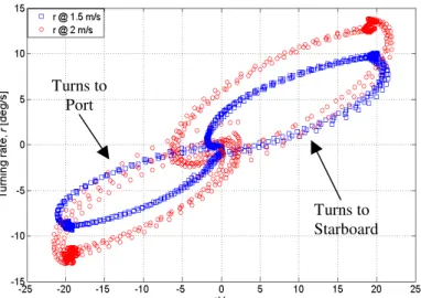
The zigzag manoeuvre is also an indicator of the efficiency of the control planes to control the vehicle’s heading [8]. The ease with which a vehicle can change its course is measured by its turning rate r, which in turn depends on the efficiency of control planes. The following figure shows the phase plane plot of yaw rate r with respect to the effective control plane yaw angle, δY. The phase plane plot was created considering only the turning regions of the trajectory where an apparent rudder deflection and a corresponding turning rate were observed.

The width of the loop indicates the stability of the vehicle. The loops for positive rudder deflections or starboard turns are wider and larger than for the port turns. This may also be as a result of the disturbance noticed in Figure 7 and Figure 8. The magnitude of the overshoot drops when stability increases but it increases when rudder efficiency increases. Thus there should be a balance between stability and rudder efficiency of a vehicle.

IV. CONCLUSIONS

In this paper, the results and observations from the horizontal zigzag manoeuvres performed using the MUN

Explorer AUV were presented. Although the results of the measured zigzag trajectory does not resemble exactly a conventional zigzag manoeuvre, it does demonstrate the ability of the AUV to precisely follow a predefined path. It was seen that the vehicle travels a considerable distance in a straight line while following the defined path. In future, experiments of this nature can be refined by adjusting the amplitude and cycle length such that the straight-line portion of the run between successive waypoints is reduced giving a more realistic zigzag manoeuvre. Although, not reported in this paper, tests 5 & 6 were an attempt to make this change by reducing the cycle length to half while maintaining the same path width.

P1

P2

P3

0o heading

Figure 9 Sketch showing the possible scenario of a cross current

cross-current

Figure 10 Phase plane plot of turning rate, r vs. δY for zigzag manoeuvres at speeds of 1.5 and 2.0 m/s (A20, L160)

Turns to Port

Turns to Starboard

ACKNOWLEDGMENT

The authors would like to thank the Natural Sciences and Engineering Research Council (NSERC) for the funding to support this research. Thanks are also due to the Atlantic Canada Opportunities Agency (ACOA) through an Atlantic Innovation Fund award to the Pan Atlantic Petroleum Systems Consortium for funding the AUV instrumentation and student funding. The team also thanks the International Submarine Engineering (ISE) for their continuing technical support.

REFERENCES

[1] E.V. Lewis, Principles of Naval Architecture, Vol. III, 1989.

[2] M. Nahon, 1996, “A Simplified Dynamics Model for Autonomous Underwater Vehicles”, Autonomous Underwater Vehicle Technology, AUV ’96, pp. 373 – 379.

[3] D. E. Perrault, 2002, “Autonomous Underwater Vehicles (AUVs) Sensitivity of Motion Response to Geometric and Hydrodynamic

Parameters and AUV Behaviors with Control Plane Faults”, Ph.D. Thesis, Memorial University of Newfoundland, February 2002. [4] J. Evans and M. Nahon, 2004, “Dynamic Modeling and Performance

Evaluation of Autonomous Underwater Vehicle, Ocean Engineering, 31, pp. 1835 – 1858.

[5] M.T. Issac, S. Adams, M. He, N. Bose, C. D. Williams, R. Bachmayer, T. Crees, “Manoeuvring Experiments Using the MUN Explorer AUV”, International Symposium on Underwater Technology, Tokyo, Japan, April 17 – 20, 2007.

[6] M.T. Issac, S. Adams, M. He, N. Bose, C. D. Williams, R. Bachmayer, T. Crees, “Manoeuvring Trials with the MUN Explorer AUV: Data Analysis and Observations”, OCEANS ‘08, Vancouver, BC, September 29 – October 4, 2007.

[7] A.C.S.AUnderwater GPS

http://www.underwater-gps.com

[8] E. Lopez, F. J. Velasco, E. Moyano, T. M. Rueda, “Full-Scale Manoeuvring Trials Simulation”, Journal of Maritime Research, Vol. 1, No. 3, pp. 37 – 50, 2004.