HAL Id: hal-01205580
https://hal.sorbonne-universite.fr/hal-01205580v2
Submitted on 18 Mar 2016
HAL is a multi-disciplinary open access
archive for the deposit and dissemination of sci-entific research documents, whether they are pub-lished or not. The documents may come from teaching and research institutions in France or
L’archive ouverte pluridisciplinaire HAL, est destinée au dépôt et à la diffusion de documents scientifiques de niveau recherche, publiés ou non, émanant des établissements d’enseignement et de recherche français ou étrangers, des laboratoires
Mathematical Analysis and Calculation of Molecular
Surfaces
Chaoyu Quan, Benjamin Stamm
To cite this version:
Chaoyu Quan, Benjamin Stamm. Mathematical Analysis and Calculation of Molecular Surfaces. Journal of Computational Physics, Elsevier, 2016, �10.1016/j.jcp.2016.07.007�. �hal-01205580v2�
Mathematical Analysis and Calculation of Molecular Surfaces
Chaoyu Quana,b, Benjamin Stammc,d
aSorbonne Universit´es, UPMC Univ Paris 06, UMR 7598, Laboratoire Jacques-Louis Lions, F-75005, Paris, France
bCNRS, UMR 7598, Laboratoire Jacques-Louis Lions, F-75005, Paris, France
cCenter for Computational Engineering Science, RWTH Aachen University, Aachen, Germany dComputational Biomedicine, Institute for Advanced Simulation IAS-5 and Institute of
Neuroscience and Medicine INM-9, Forschungszentrum J¨ulich, Germany
Abstract
In this article we derive a complete characterization of the Solvent Excluded Surface (SES) for molecular systems including a complete characterization of singularities of the surface. The theory is based on an implicit representation of the SES, which, in turn, is based on the signed distance function to the Solvent Accessible Surface (SAS). All proofs are constructive so that the theory allows for efficient algorithms in order to compute the area of the SES and the volume of the SES-cavity, or to visualize the surface. Further, we propose to refine the notion of SAS and SES in order to take inner holes in a solute molecule into account or not.
Keywords: Molecular surface, solvent excluded surface, solvation models,
mathematical description, constructive algorithm
1. Introduction
The majority of chemically relevant reactions take place in the liquid phase and the effect of the environment (solvent) is important and should be considered in various chemical computations. In consequence, a continuum solvation model is a model in which the effect of the solvent molecules on the solute are described by a continuous model [21]. In continuum solvation continuum models, the notion of molecular cavity and molecular surface is a fundamental part of the model. The molecular cavity occupies the space of the solute molecule where a solvent molecule cannot be present and the molecular surface, the boundary of the corresponding cavity, builds the interface between the solute and the solvent respectively between the continuum and the atomistic description of the physical model. A precise under-standing of the nature of the surface is therefore essential for the coupled model and
in consequence for running numerical computations. The Van der Waals (VdW) sur-face, the Solvent Accessible Surface (SAS) and the Solvent Excluded Surface (SES) are well-established concepts. The VdW surface is more generally used in chemical calculations, such as in the recent developments [4, 14] for example, of numerical approximations to the COnductor-like Screening MOdel (COSMO) due to the sim-plicity of the cavity. Since the VdW surface is the topological boundary of the union of spheres, the geometric features are therefore easier to understand. However, the SES, which is considered to be a more precise description of the cavity, is more complicated and its analytical characterization remains unsatisfying despite a large number of contributions in literature.
1.1. Previous Work
In quantum chemistry, atoms of a molecule can be represented by VdW-balls with VdW-radii obtained from experiments [17]. The VdW surface of a solute molecule is consequently defined as the topological boundary of the union of all VdW-balls. For a given solute molecule, its SAS and the corresponding SES were first introduced by Lee & Richards in the 1970s [13, 18], where the solvent molecules surrounding a solute molecule are reduced to spherical probes [21]. The SES is also called “the smooth molecular surface” or “the Connolly surface”, due to Connolly’s fundamen-tal work [7]. He has divided the SES into three types of patches: convex spherical patches, saddle-shaped toroidal patches and concave spherical triangles. But the self-intersection among different patches in this division often causes singularities despite that the whole SES is smooth almost everywhere. This singularity problem has led to difficulty in many associated works with the SES, for example, failure of SES meshing algorithms and imprecise calculation of molecular areas or volumes, or has been circumvented by approximate techniques [6]. In 1996, Michel Sanner treated some special singularity cases in his MSMS (Michel Sanner’s Molecular Sur-face) software for meshing molecular surfaces [20]. However, to our knowledge, the complete characterization of the singularities of the SES remains unsolved.
1.2. Contribution
In this paper, we will characterize the above molecular surfaces with implicit functions, as well as provide explicit formulas to compute analytically the area of molecular surfaces and the volume of molecular cavities. We first propose a method to compute the signed distance function to the SAS, based on three equivalence
statements which also induce a new partition of R3. In consequence, a computable
implicit function of the corresponding SES is given from the relatively simple re-lationship between the SES and the SAS. Furthermore, we will redefine different
types of SES patches mathematically so that the singularities will be characterized explicitly. Besides, by applying the Gauss-Bonnet theorem [8] and the Gauss-Green theorem [10], we succeed to calculate analytically all the molecular areas and vol-umes, in particular for the SES. These quantities are thought to be useful in protein modeling, such as describing the hydration effects [19, 3].
In addition, we will refine the notion of SAS and SES by considering the possible inner holes in the solute molecule yielding the notions of the complete SAS (cSAS) and the corresponding complete SES (cSES). To distinguish them, we call respec-tively the previous SAS and the previous SES as the exterior SAS (eSAS) and the exterior SES (eSES). A method with binary tree to construct all these new molecular surfaces will also be proposed in this paper in order to provide a computationally efficient method.
1.3. Outline
We first introduce the concepts of implicit surfaces in the second section and the implicit functions of molecular surfaces are given in the third section. In the fourth section, we present two more precise definitions about the SAS, either by taking the inner holes of the solute molecule considered into account or not. Then, based on three equivalence statements that are developed, we propose a computable method to calculate the signed distance function from any point to the SAS analytically. In this process, a new Voronoi-type diagram for the SAS-cavity is given which allows us to calculate analytically the area of the SAS and the volume inside the SAS. In the fifth section, a computable implicit function of the SES is deduced directly from the signed distance function to the SAS and according to the new Voronoi-type diagram, all SES-singularities are characterized. Still within this section, the formulas of calculating the area of the SES and the volume inside the SES will be provided. In the sixth section, we explain how to construct the SAS (cSAS and eSAS) and the SES (cSES and eSES) for a given solute molecule considering the possible inner holes. Numerical results are illustrated in the seventh section and finally, we provide some conclusions of this article in the last section.
2. Introduction to Implicit Surfaces
We start with presenting the definition of implicit surfaces [22]. In a very general
context, a subset O ⊂ Rn is called an implicit object if there exists a real-valued
function f : U → Rkwith O ⊂ U ⊂ Rn, and a subset V ⊂ Rk, such that O = f−1(V ).
That is,
The above definition of an implicit object is broad enough to include a large family of
subsets of the space. In this paper, we consider the simple case where U = R3, V =
{0} and f : R3 → R is a real-valued function. In consequence, an implicit object is
represented as a zero-level set O = f−1(0), which is also called an implicit surf ace in
R3, and the function f is called an implicit f unction of the implicit surface. Notice
that there are various implicit functions to represent one surface in the form of a zero-level set.
The signed distance function fS of a closed bounded oriented surface S in R3,
determines the distance from a given point p ∈ Rn to the surface S, with the sign
determined by whether p lies inside S or not. That is to say,
fS(p) = − inf x∈Skp − xk if p lies inside S, inf x∈Skp − xk if p lies outside S. (2.1)
This is naturally an implicit function of S. 3. Implicit Molecular Surfaces
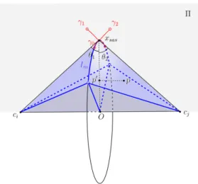
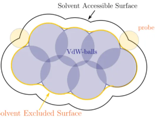
In quantum chemistry, atoms of a molecule are represented by VdW-balls with VdW radii which are experimentally fitted, given the underlying chemical element [17]. In consequence and mathematically speaking, the VdW surface is defined as the topological boundary of the union of all VdW-balls. Besides, the SAS of a solute molecule is defined by the center of an idealized spherical probe rolling over the solute molecule, that is, the surface enclosing the region in which the center of a spherical probe can not enter. Finally, the SES is defined by the same spherical probe rolling over the solute VdW-cavity, that is, the surface enclosing the region in which a spherical probe can access. In other words, the SES is the boundary of the union of all spherical probes that do not intersect the VdW-balls of the solute molecule, see Figure 1 for a graphical illustration.
We denote by M the number of atoms in a solute molecule, by ci ∈ R3and ri ∈ R+
the center and the radius of the i-th VdW atom. The open ball with center ci and
radius ri is called the i-th VdW-ball. The Van der Waals surface can consequently
be represented as an implicit surface fvdw−1(0) with the following implicit function:
fvdw(p) = min
i=1,...,M{kp − cik2 − ri}, ∀p ∈ R
3. (3.2)
Similarly, the open ball with center ci and radius ri+ rp is called the i-th SAS-ball
Figure 1: This is a 2-dimension (2D) schematics of the Solvent Accessible Surface and the Solvent Excluded Surface, both defined by a spherical probe in orange rolling over the molecule atoms in dark blue.
we denote by Si the i-th SAS-sphere corresponding to Bi, that is, Si = ∂Bi. Similar
to the VdW surface, the SAS can be represented as an implicit surface fe−1
sas(0) with
the following implicit function:
e
fsas(p) = fvdw(p) − rp = min
i=1,...,M{kp − cik2 − ri− rp}, ∀p ∈ R
3. (3.3)
We notice that the above implicit function of the SAS is simple to compute. It seems nevertheless hopeless to us to further obtain an implicit function of the SES
if constructing upon this simple implicit function fesas(p) which is not a distance
function. On the other hand, having the signed distance function, see (2.1), at hand would allow the construction of an implicit function for the SES due to the geometrical relationship between the SAS and the SES.
Indeed, according to the fact that any point on the SES has signed distance −rp
to the SAS, an implicit function of the SES is obtained directly as:
fses(p) = fsas(p) + rp, (3.4)
which motivates the choice of using the signed distance function to represent the
SAS. From the above formula, the SES can be represented by a level set fsas−1(−rp),
associated with the signed distance function fsas to the SAS. Therefore, the key point
becomes how to compute the signed distance fsas(p) from a point p ∈ R3 to the SAS.
Generally speaking, given a general surface S ⊂ R3 and any arbitrary point p ∈ R3,
it is difficult to compute the signed distance from p to S. However, considering that the SAS is a special surface formed by the union of SAS-spheres, this computation can be done analytically.
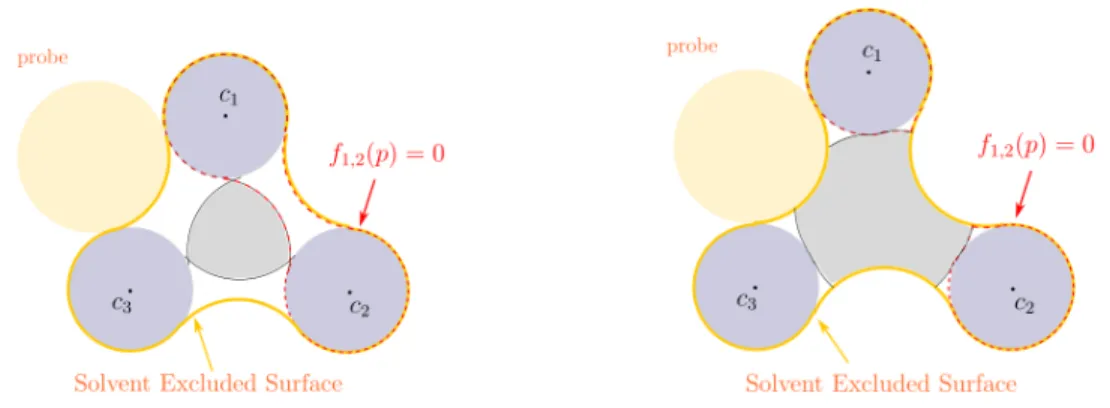
Figure 2: The above figures illustrate two SESs of two artificial molecules respectively containing three atoms. In each of them, f1,2 denotes the signed distance function to the SES of the 1-th and the 2-th atoms which is depicted with dashed red curves (f2,3 and f1,3 are similar).
We state a remark about another implicit function to characterize the SES, pro-posed by Pomelli and Tomasi [16]. In [15], this function can be written as:
e
fses(p) = min
1≤i<j<k≤Mfijk(p), ∀p ∈ R 3
, (3.5)
where fijk represents the signed distance function to the SES of the i-th, j-th and
k-th VdW atom. However, this representation might fail sometimes, see two repre-sentative 2D examples in Figure 2. Indeed, the formula (3.5) for each molecule in Figure 2 can be rewritten as:
e
fses(p) = min
1≤i<j≤3fi,j(p), ∀p ∈ R 2,
(3.6)
where fi,j represents the signed distance function to the SES of the i-th and the j-th
VdW atom. However, each molecular cavity defined by {p ∈ R2 : fe
ses(p) ≤ 0} has
excluded the region in grey inside the real SES.
Further, the region enclosed by the Van der Waals surface is called the
VdW-cavity, that is, any point p in the VdW-cavity satisfies fvdw(p) ≤ 0. More generally,
we call the region enclosed by a molecular surface as the corresponding molecular cavity. In consequence, the region enclosed by the SAS is called the SAS-cavity, and the region enclosed by the SES is called the SES-cavity. Similarly, any point p
in the SAS-cavity satisfies fsas(p) ≤ 0, and any point p in the SES-cavity satisfies
fses(p) ≤ 0.
4. The Solvent Accessible Surface
In the framework of continuum solvation models, using the VdW-cavity as the solvent molecular cavity has the characteristic that its definition does not depend
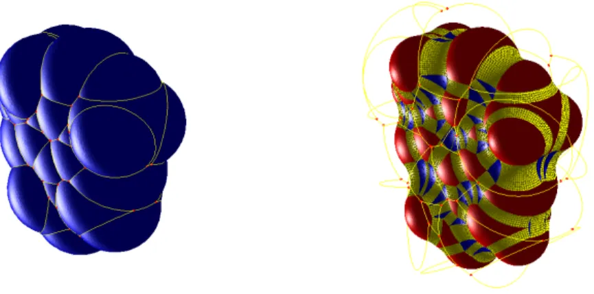
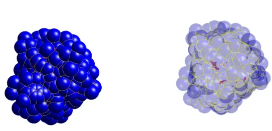
Figure 3: The left figure shows the components of the eSAS of the protein 1B17 (the probe radius rp = 1.2˚A): open spherical patches in blue, open circular arcs in yellow and intersection points in red. The right figure shows the exterior surface (transparent) and the interior surfaces of the eSES of the protein 1B17. The boundary of an exterior spherical patch of the eSAS is composed of circular arcs depicted in yellow, and the boundary of an interior spherical patch of the cSAS is composed of circular arcs depicted in purple.
in any way on characteristics of the solvent. In other words, the above-mentioned VdW surface has ignored the size and shape of the solvent molecules, while the definition of the Solvent Accessible Surface includes some of these characteristics. In the following, we first provide two more precise mathematical definitions of the SAS considering possible inner holes of a solute molecule. After that, we will provide a formula for the signed distance function to the SAS, which is indeed based on three equivalence statements, providing explicitly a closest point on the SAS to any point
in R3. In this process, a new Voronoi-type diagram will be proposed to make a
partition of the space R3, which, in turn, will also be used to calculate the exact
volume of the SAS-cavity. 4.1. Mathematical Definitions
In [13], the Solvent Accessible Surface is defined by the set of the centers of the spherical probe when rolling over the VdW surface of the molecule. At first glance, one could think that it can equivalently be seen as the topological boundary of the union of all SAS-balls of the molecule. However, we notice that there might exist some inner holes inside the molecules where a solvent molecule can not be present. In consequence, the SAS may or may not be composed of several separate surfaces,
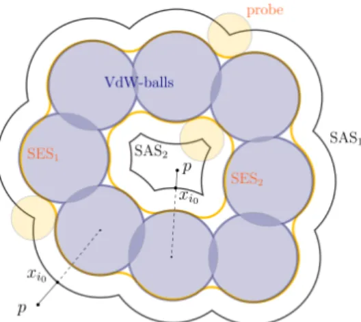
Figure 4: This is a 2D schematic of different molecular surfaces, including the VdW surface, the cSAS, the eSAS, the cSES and the eSES. The yellow discs denote the probes, representing solvent molecules, while the blue discs denote the VdW-balls. SAS1 is the trace of the probe center when a probe rolls over the exterior of the VdW-balls, while SAS2 is the trace of the probe center when a probe rolls over the inner holes of the VdW-balls. SES1 and SES2 respectively denote the corresponding solvent excluded surfaces to SAS1 and SAS2. The cSAS is the union of SAS1 and SAS2, while the eSAS is just SAS1. Similarly, the cSES is the union of SES1 and SES2, while the eSES is just SES1. Finally, xi0 is a closest point on the SAS to a given point p.
see Figure 3 for a graphical illustration. This inspires us to propose two more precise surfaces: the complete Solvent Accessible Surface (cSAS) defined simply as the boundary of the union of the SAS-balls, and the exterior Solvent Accessible Surface (eSAS) defined as the outmost surface obtained when a probe rolls over the exterior of the molecule, see Figure 4. In the case where there are no interior holes inside the molecule, the cSAS and the eSAS will coincide. We make a convention that the SAS refers to both the cSAS and the eSAS in a general context.
Since both the cSAS and the eSAS are two closed sets, there exists a closest point
on the SAS to any given point p ∈ R3, which is denoted by xp
sas. Thus, the signed
distance function fsas can be written as:
fsas(p) =
(
−kp − xp
sask if p lies inside the SAS,
kp − xp
sask if p lies outside the SAS.
(4.7)
In the above formula, xpsas depends on p. When p lies on the SAS, p coincides with
xp
sas and fsas(p) = 0. It remains therefore to find a closest point xpsas on the SAS
to the given point p ∈ R3. Note that there might exist more than one closest point
on the SAS to the point p and xpsas is chosen as one of them. In the context, this is
way to calculate analytically a closest point on the SAS to a given point p, based on three equivalence statements.
4.2. Equivalence Statements
According to the definitions of the cSAS and the eSAS, these two molecular surfaces are both composed of three types of parts: open spherical patches, open circular arcs and intersection points (formed by the intersection of at least three SAS-spheres), see Figure 3. Note that an SAS intersection point can in theory be formed by the intersection of more than three SAS-spheres. However, these cases can be divided into multiple triplets of SAS-spheres for simplicity as mentioned in [12]. In this spirit, we make an assumption that all SAS intersection points are formed by the intersection of three SAS-spheres. Furthermore, we assume that any SAS-ball is not included by any other (otherwise, the inner SAS-ball can be ignored) In the following analysis.
For an SAS, denote by m1 the number of the SAS spherical patches, by m2 the
number of the SAS circular arcs, and by m3 the number of the SAS intersection
points. Then, denote by Pm the m-th SAS spherical patch on the SAS where m =
1, . . . , m1. Denote by lmthe m-th SAS circular arc on the SAS where m = 1, . . . , m2.
Denote by xm the m-th SAS intersection point on the SAS where m = 1, . . . , m3.
Furthermore, denote by I the set of all SAS intersection points written as:
I = {xm : m = 1, . . . , m3} = {x ∈ SAS : ∃ 1 ≤ i < j < k ≤ M, s.t. x ∈ Si∩Sj∩Sk}.
With the above notations, we consider to calculate a closest point on the SAS to a given point p in the case when p lies outside the SAS (the cSAS or the eSAS). Lemma 4.1. Let the point p lie outside the SAS (the cSAS or the eSAS), i.e. kp − cik ≥ ri+ rp, ∀1 ≤ i ≤ M . Further, let i0 ∈ {1, . . . , M } be such that
kp − ci0k − (ri0 + rp) = min1≤i≤M{kp − cik − (ri+ rp)}. (4.8)
Then, the point
xi0 = ci0 + (ri0 + rp)
p − ci0 kp − ci0k
, (4.9)
is the closest point to p on the SAS and fsas(p) = kp − xi0k = min
1≤i≤M{kp − cik − (ri+ rp)}. (4.10)
So far, we have discussed the case when p lies outside the SAS (both the cSAS and the eSAS), which is not too difficult to deal with. Next, we need to consider the case where p lies inside the (complete or exterior) SAS-cavity, to obtain the signed
distance function fsas(p) from any point p ∈ R3 to the SAS. The following analysis
can be applied to both the cSAS and the eSAS. This problem is handled inversely, in the sense that we will determine the region in the molecular cavity for an arbitrary
given point xsas ∈ SAS, such that xsas is a closest point to any point in this region.
To do this, we first define a mapping R : X 7→ Y , where X is a subset of the SAS, and Y = R(X) is the region in the SAS-cavity, such that there exists a closest point in X on the SAS to any point in Y . That is,
Y = {y : y lies in the SAS-cavity and ∃ xysas ∈ X s.t. xy
sas is a closest point to y}.
In the following, we propose three equivalence statements between a point xsas
on the SAS and the corresponding region R(xsas) for three cases where xsas lies
respectively on the three different types of the SAS. We recall first, however, a useful inequality between two signed distance functions to two surfaces.
Proposition 4.1. Consider two bounded, closed and oriented surfaces S ⊂ R3 and
S0 ⊂ R3 with two corresponding signed distance functions f
S(p) and fS0(p). If the
cavity inside S is contained in the cavity inside S0, then we have fS0(p) ≤ fS(p),
∀p ∈ R3.
With the above proposition, we propose first a result which connects a point on an SAS spherical patch with a closed line segment in the SAS-cavity.
Theorem 4.1. Assume that p ∈ R3 is a point in the SAS-cavity and x
sas is a point
on the SAS. If xsas is on an SAS spherical patch Pm on the i-th SAS-ball Si, then
xsas is a closest point on the SAS to p if and only if p lies on the closed line segment
[ci, xsas]. That is, R(xsas) = [ci, xsas]. Further, the closest point xsas on the SAS is
unique if and only if p 6= ci. If p = ci, then any point on Pm is a closest point to p.
Proof. First suppose that xsas is a closest point to p with xsas ∈ Pm ⊂ Si. Since Pm
is an open set, take a small enough neighborhood V of xsas such that V ⊂ Pm, see
Figure 5, and since xsas is a closest point on the SAS to p, we have
kp − xsask ≤ kp − xk, ∀x ∈ V, (4.11)
which yields that the vector from xsas to p is perpendicular to any vector in the
tangent plane of Si at xsas, thus the vector from p to xsas is the normal vector at xsas
Figure 5: Illustration when the point xsas lies on an SAS spherical patch Pm which is part of an SAS-sphere Si, and p lies on the segment [ci, xsas]. V represents a neighborhood of xsas on the spherical patch. αs is the angle variation at the vertex vs between two neighboring circular arcs es−1and es on the boundary of this spherical patch.
of Si. Furthermore, from the convexity of Pm, p has to lie on the closed line segment
[ci, xsas].
On the other hand, suppose that xsas ∈ Pm ⊂ Si, and p ∈ [ci, xsas]. In
conse-quence, xsas is obviously a closest point on the sphere Si to p, see Figure 5. The
signed distance function fSi(p) is equal to −kp − xsask. Notice that the cavity inside
Si, i.e. Bi, is contained in the SAS-cavity. We can then use Proposition 4.1 by taking
S as Si and S0 as the SAS, to obtain fsas(p) ≤ fSi(p) = −kp − xsask. Therefore, we
have
−kp − xk ≤ fsas(p) ≤ −kp − xsask, ∀x ∈ SAS. (4.12)
That is, kp − xk ≥ kp − xsask, ∀x ∈ SAS, which means that xsas is a closest point
on the SAS to p.
Finally, assume that p ∈ [ci, xsas]. If p = ci, then any point on Pmis a closest point
to p because the distance is uniformly kci− xsask = ri+ rp. If p 6= ci, then the open
ball Br(p) with r = kp − xsask < ri+ rp is included in Bi and ∂Br(p) ∩ Si = {xsas},
which implies that xsas is the unique closest point to p.
Next, we propose another equivalence statement, which connects a point on an SAS circular arc with a closed triangle in the SAS-cavity.
Theorem 4.2. Assume that p ∈ R3 is a point in the SAS-cavity and x
sas is a point
on the SAS. If xsas is on an SAS circular arc lm associated with Si and Sj, then xsas
is a closest point on the SAS to p if and only if p lies in the closed triangle 4xsascicj
defined by three vertices xsas, ci and cj. That is, R(xsas) = 4xsascicj. Further, the
closest point xsas on the SAS is unique if and only if p does not belong to the edge
Proof. First suppose that xsas is a closest point to p with xsas ∈ lm ⊂ Si∩ Sj. Since
lm is an open circle arc on the circle Si∩ Sj, take a small enough neighboring curve
γ0 of xsas with γ0 ⊂ lm, see Figure 6. Since xsas is a closest point to p, we have
kp − xsask ≤ kp − xk, ∀x ∈ γ0. (4.13)
Denote by p0 the projection of p onto the plane where lm lies. By substituting
kp − xsask2 = kp − p0k2+ kp0− xsask2 and kp − xk2 = kp − p0k2+ kp0 − xk2 into the
inequality (4.13), we obtain that
kp0− xsask ≤ kp0− xk, ∀x ∈ γ0, (4.14)
which yields that the vector from xsas to p0 is perpendicular to the tangent vector
of γ0 at xsas. In consequence, p0 has to lie on the ray Oxsas starting from O and
passing through xsas, where O is the center of the circular arc lm. Thus, p must
lie on the closed half plane Π defined by the three points xsas, ci and cj and whose
boarder is the line passing through ci and cj. The closed half plane Π contains the
ray Oxsas and is perpendicular to the plane where lm lies. We then take another two
neighboring curves γ1 and γ2 of xsas, with γ1 ⊂ Π ∩ Si∩ SAS and γ2 ⊂ Π ∩ Sj∩ SAS,
see Figure 6. In this case, γ1 has one closest endpoint xsas and is open at the other
end, which is the same for γ2. From the assumption that xsas is a closest point on
the SAS to p, we have the following inequality
kp − xsask ≤ kp − xk, ∀x ∈ γ1∪ γ2. (4.15)
This yields that p ∈ 4xsascicj, where 4xsascicj is the closed triangle on Π with three
vertices xsas, ci and cj. Otherwise, we can find a point x ∈ (γ1 ∪ γ2)\xsas strictly
closer to p than xsas, which contradicts the assumption.
On the other hand, suppose that p ∈ 4xsascicj. In consequence, it is not difficult
to obtain that xsas is the closest point to p on ∂(Bi∪ Bj), where Bi and Bj are the
corresponding SAS-balls corresponding to Si and Sj as mentioned above. Similarly,
we know that the signed distance function f∂(Bi∪Bj)(p) is equal to −kp − xsask, and
notice that Bi ∪ Bj is contained in the SAS-cavity. We can use again Proposition
4.1, by taking S as ∂(Bi∪ Bj) and S0 as the SAS, to obtain fsas(p) ≤ f∂(Bi∪Bj)(p) =
−kp − xsask. Therefore, we have
−kp − xk ≤ fsas(p) ≤ −kp − xsask, ∀x ∈ SAS. (4.16)
That is, kp − xk ≥ kp − xsask, ∀x ∈ SAS, which means that xsas is a closest point
Figure 6: Illustration when lm is an SAS circular arc associated with two SAS-spheres Si and Sj. The point xsason lm is a closest point on the SAS to p. γ0 is a small neighborhood of xsas on the circular arc lm, whereas γ1and γ2 represent two small neighboring curves of xsason the SAS, with xsas as the endpoints, γ1⊂ Π ∩ Si∩ SAS, and γ2⊂ Π ∩ Sj∩ SAS.
If p ∈ [ci, cj], then any point on lm is a closest point to p since the distance from
any point on lm to p is constant. If p ∈ 4xsascicj\[ci, cj], then the open ball Br(p)
with r = kp − xsask < ri+ rp is included in Bi∪ Bj and ∂Br(p) ∩ ∂(Bi∪ Bj) = {xsas},
which implies that xsas is the unique closest point to p.
By mapping with R a whole SAS spherical patch Pm to the SAS-cavity, we obtain
a spherical sector R(Pm) in the SAS-cavity with cap Pm, center ci and radius ri+ rp,
see Figure 5. Similarly, by mapping with R a whole SAS circular arc lm to the
SAS-cavity, we obtain a double-cone region R(lm) in the SAS-cavity with the circular
sector corresponding to lm as base, ci and cj as vertices, see Figure 6.
Removing now the above-mentioned spherical sectors and double-cone regions from the SAS-cavity, the closed hull of the remaining region, denoted by T , is conse-quently a collection of closed separate polyhedrons, see an example of three atoms in
Figure 7. Each polyhedron is denoted by Tn with index n and thus T =STn.
Con-sidering now the last case where xsas is an SAS intersection point xm, we have a third
equivalence statement as a corollary of the previous two equivalence statements.
Corollary 4.1. If xsas is an SAS intersection point xm ∈ I associated with Si, Sj
and Sk, then xsas is a closest point on the SAS to p if and only if p lies in the closed
region T and xsas is a closest point in I to p.
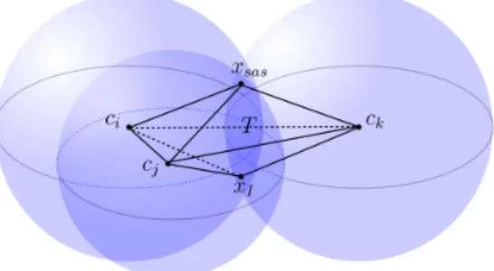
Figure 7: This figure illustrates the closed region T of three SAS-spheres with the centers (ci, cj, ck), where the tetrahedron T has five vertices (xsas, ci, cj, ck, xI). Here, xsas is one SAS intersection point in I, and xI is the other SAS intersection point.
of its corresponding region in the SAS-cavity as following:
R(xm) = T ∩ {p : kp − xmk ≤ kp − xk, ∀x 6= xm, x ∈ I}. (4.17)
It is not difficult to find that R(xm) is a closed polyhedron. At the same time,
mapping I into the SAS-cavity with R, we obtain R(I) = T .
With the three equivalence statements as well as the above-defined map R, we obtain in fact a non-overlapping decomposition of the SAS-cavity, including spherical sectors, double-cone regions and polyhedrons. It should be emphasized that given a
point p ∈ R3 contained in the SAS-cavity and known the region where p lies, we can
then calculate a closest point xpsas on the SAS to p according to this decomposition.
The signed distance function fsas(p) can therefore be calculated analytically by the
formula 4.7, which, in turn, will ultimately provide an implicit function of the SES. In the next subsection, we will investigate further in the partition of the SAS-cavity based on the above equivalence statements, in order to compute efficiently the area of the SAS and the volume of the SAS-cavity.
4.3. New Voronoi-type Diagram
The above non-overlapping decomposition of the SAS-cavity can also be seen as a new Voronoi-type diagram, which will be presented comparing with the well-known Voronoi Diagram and the Power Diagram recalled in the following.
a.. Voronoi Diagram
The Voronoi diagram [9] was initially a partition of a 2D plane into regions based on the distance to points in a specific subset of the plane. In the general case, for
an Euclidean subspace X ⊂ Rn endowed with a distance function d and a tuple of
of all points in X whose distance to Ai is not greater than their distance to any other
set Aj for j 6= i. In other words, with the distance function between a point x and
a set Ai defined as
dV(x, Ai) = inf
y∈X {d(x, y) | y ∈ Ai},
the formula of the Voronoi region Ri is then given by:
Ri = {x ∈ X | dV(x, Ai) ≤ dV(x, Aj) , ∀ j 6= i}. (4.18)
Most commonly, each subset Ai is taken as a point and its corresponding Voronoi
region Ri is consequently a polyhedron, see an example of three points in R2 in
Figure 8.
b.. Power Diagram
In computational geometry, the power diagram [1], also called the Laguerre-Voronoi diagram, is another partition of a 2D plane into polygonal cells defined from a set of circles in R2. In the general case, for a set of circles (Ci)i∈K (or spheres) in
Rn with n ≥ 2, the power region Ri associated with Ci consists of all points whose
power distance to Ci is not greater than their power distance to any other circle Cj,
for j 6= i. The the power distance from a point x to a circle Ci with center ci and
radius ri is defined as
dP(x, Ck) = kx − ckk2− rk2,
the formula of the Power region Ri is then given by:
Ri = {x ∈ Rn| dP(x, Ci) ≤ dP(x, Cj) , ∀ j 6= i}.
The power diagram is a form of generalized Voronoi diagram, in the sense that you
can take the circles Ci instead of the centers ci and simply replace the distance
function dV in the Voronoi diagram with the power distance function dP, to obtain
the power diagram, see an example of three circles in R2 in Figure 8. Notice that
the power distance is not a real distance function. By summing up the volume of each power region inside the SAS-cavity, one can calculate the exact volume of the cSAS-cavity, which is equivalent to calculate the volume of the union of balls, see [2, 5].
c.. New Voronoi-Type Diagram
In this paper, we propose a new Voronoi-type diagram for a set of spheres in R3
(or circles in R2), which is inspired by the non-overlapping decomposition of the
volume of the (complete or exterior) SAS-cavity, but also the (complete or exterior) SES-cavity which will be defined in the next section.
We first look at the new Voronoi-type diagram for a set of discs in the case of 2D. Notice that the boundary γ of the union of these discs can be classified into two types: open circular arcs {l1, l2, . . . , ln} and intersection points {x1, x2, . . . , xn}, with
the number of circular arcs equal to the number of intersection points. Take A1 =
l1, . . . , An = ln, An+1 = {x1, x2, . . . , xn} in the Voronoi diagram. In consequence,
we obtain n + 1 corresponding new Voronoi-type regions {R1, . . . , Rn, Rn+1}, where
Ri is given by (4.18).
From a similar mapping R and similar equivalence theorems, we know that the
part of Ri inside γ is a circular sector when 1 ≤ i ≤ n, and Rn+1 is the remaining
region composed of polygons, see an example of three circles in Figure 8. For any
point x ∈ R2, we have x ∈ R
i if and only if there exists a point in Ai such that it is
a closet point to x on γ.
In the 3D case, the SAS consists of three types of geometrical quantities: open spherical patches, open circular arcs and intersection points. Similarly to the case in 2D, we take A1 = P1, . . . , Am1 = Pm1, Am1+1 = l1, . . . , Am1+m2 = lm2 and Am1+m2+1 = {x1, . . . , xm3} with the above-mentioned notations. In consequence, we
obtain m1 + m2 + 1 corresponding new Voronoi-type regions
{R1, . . . , Rm1, Rm1+1, . . . , Rm1+m2, Rm1+m2+1}.
With the mapping R defined in the last section, we know that the spherical
sector R(Pm) corresponds to Rm in the SAS-cavity, the double-cone region R(lm)
corresponds to Rm1+m in the SAS-cavity, and the closed region R(I) coincides with
Rm1+m2+1. For any point x ∈ R
3, we have x ∈ R
i if and only if there exists a point
in Ai such that it is a closet point on the SAS to x. The new Voronoi-type diagram
is a powerful tool for calculating analytically the molecular area and volume, which is a direct consequence of the three equivalence statements. Given the components of the SAS, the new Voronoi-type diagram can be obtained directly according to the three equivalence statements, while the power diagram needs more complicated computations.
4.4. SAS-Area and SAS-Volume
In this paper, the area of the SAS is called the SAS-area and the volume of the SAS-cavity is called the SAS-volume. Similarly, the area of the SES is called the SES-area and the volume of the SES-cavity is called the SES-volume. Next, we will use the Gauss-Bonnet theorem of differential geometry to calculate the SAS-area, and then will use the new Voronoi-type diagram to calculate the SAS-volume.
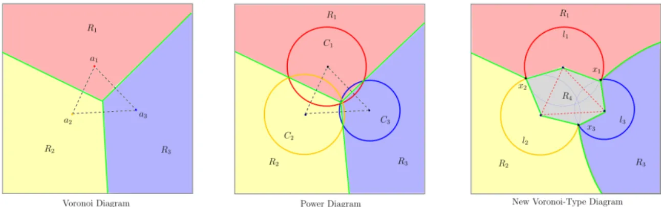
Figure 8: The left figure gives the Voronoi diagram of three points {a1, a2, a3} in R2. R1 is the Voronoi region associated with a1, while R2 associated with a2 and R3 associated with a3. The middle figure gives the power diagram of three circles {C1, C2, C3} in R2, with three corresponding power regions R1, R2and R3. The right figure gives the new Voronoi-type diagram of three circles in R2, with four regions R1, R2, R3and R4respectively corresponding to l1, l2, l3and {x1, x2, x3}.
a.. SAS-Area
To calculate analytically the solvent accessible area, the Gauss-Bonnet theorem has already been applied in the 1980s [7], which allows one to calculate the area of each SAS spherical patch with the information along its boundary, and then sum them up. We introduce briefly the key formula used in this calculation to keep the article complete. The area of a spherical patch P can be obtained from the Gauss-Bonnet theorem as following (see Figure 5):
X i αi+ X i kei|ei| + 1 r2AP = 2πχ, (4.19)
where αi is the angle at the vertex vi on the boundary between two neighboring
circular arcs ei−1 and ei, kei is the geodesic curvature of the edge ei, |ei| is the length of this edge ei and AP is the area of the patch P . Finally, χ is the Euler characteristic
of P , which is equal to 2 minus the number of loops forming the boundary of P .
Through the above formula, we calculate the area of each SAS spherical patch APm
and sum them up to get the SAS-area Asas:
Asas = m1 X m=1 APm. (4.20) b.. SAS-Volume
In the new Voronoi-type diagram, the SAS-cavity is decomposed into three types of region: spherical sectors, double-cone regions and polyhedrons. For a spherical
patch Pm on Si with center ci and radius ri + rp, the volume of the corresponding
spherical sector R(Pm), denoted by VPm, can be calculated as following:
VPm = 1
3APm(ri+ rp).
For a circular arc lm associated with Si and Sj (see Figure 6), the volume of the
cor-responding double-cone region R(lm), denoted by Vlm, can be calculated as following:
Vlm = 1
6rlm|lm| kci− cjk.
where rlm is the radius of this circular arc and |lm| is the length of lm. Finally, the volume of the closed region T = R(I) can be calculated according the Gauss-Green theorem [10]:
VT =
X
t
At(nt· n0),
where t denotes a triangle on the boundary of T , At is the area of the triangle t, nt
is the outward pointing normal vector of t and n0 is an arbitrary given unit direction
vector in R3, for example, n0 = (1, 0, 0).
From the above three formulas, we sum up the volume of each spherical sector, each double-cone region and the polyhedron T , to get the solvent accessible volume Vsas as below: Vsas = 1 3 m1 X m=1 APm(ri + rp) + 1 6 m2 X m=1 rlm|lm| kci− cjk + X t At(nt· n0). (4.21)
5. The Solvent Excluded Surface
The Solvent Excluded Surface was first proposed by Lee & Richards in the 1970s [18]. Although the SES is believed to give a more accurate description of the molecu-lar cavity, it is more complicated than the other two molecumolecu-lar surfaces. We first give two more precise definitions of the SES considering inner holes of a molecule. After that, we define mathematically different types of patches on the SES, which helps us to characterize and calculate analytically singularities on the SES. Finally, com-bining the above-proposed new Voronoi-type diagram and the upcoming singularity analysis, we calculate the exact SES-area and the SES-volume.
5.1. Mathematical Definitions
In previous works [13, 18], the SES is defined as the topological boundary of the union of all possible spherical probes that do not intersect any VdW atom of the molecule. In other words, the SES is the boundary of the cavity where a spherical probe can never be present. However, there might exist inner holes inside the so-lute molecule. Similar to the definitions of the cSAS and the eSAS, the complete Solvent Excluded Surface (cSES) is defined as the set of all points with signed
distance −rp to the cSAS, while the exterior Solvent Excluded Surface (eSES)
is defined as the set of all points with signed distance −rp to the eSAS. We make
a similar convention as before that the SES refers to both the cSES and the eSES.
From the geometrical relationship between the SAS and the SES, i.e. SES = fsas−1(rp),
we propose an implicit function of the SES: fses(p) = ( −kp − xp sask + rp if fsas(p) ≤ 0, kp − xp sask + rp if fsas(p) ≥ 0, (5.22) where xp
sas is a closest point on the SAS to p, which depends on p and can be obtained
directly from the equivalence statements.
In Connolly’s work [7], the SES is divided into three types of patches: convex spherical patches, saddle-shaped toroidal patches and concave spherical triangles, see Figure 9. The convex spherical patches are the remainders of VdW-spheres, which occur when the probe is rolling over the surface of an atom and touches no other atom. The toroidal patches are formed when the probe is in contact with two atoms at the same time and rotates around the axis connecting the centers of these two atoms. While rolling, the probe traces out small circular arcs on each of the two VdW-spheres, which build the boundaries between the convex spherical patches and the toroidal patches. The concave spherical triangles occur if the probe is simultaneously in contact with more than or equal to three VdW-spheres. Here, the probe is in a fixed position, meaning that it is centered at an SAS intersection point and cannot roll without losing contact to at least one of the atoms.
The intersection between different SES patches might occur which leads to singu-larities on the SES, referred to as SES-singusingu-larities, see Figure 10. Despite some par-ticular cases which have been studied by Sanner [20], a characterization of these sin-gularities is not known. We will provide a complete characterization, using the above equivalence statements as well as the following analysis of the SES-singularities. To start with, we give three new definitions of different SES patches from the mathe-matical point of view:
1) Convex Spherical Patch: A convex spherical patch on the SES, denoted
Figure 9: The above figures show both the SAS and the SES of the caffeine molecule (the probe radius rp = 1.2˚A). On the left, the SAS is composed of spherical patches in blue, circular arcs in yellow and intersection points in red. On the right, the patches in red (resp. in yellow or in blue) are the corresponding convex spherical patches (resp. toroidal patches or concave spherical patches) on the SES.
a closest point on the SAS belonging to a common SAS spherical patch Pm,
where 1 ≤ m ≤ m1.
2) Toroidal Patch: A toroidal patch on the SES, denoted by Pt, is defined as
the set of the points on the SES such that there exists a closest point on the
SAS belonging to a common SAS circular arc lm, where 1 ≤ m ≤ m2.
3) Concave Spherical Patch: A concave spherical patch on the SES, denoted
by P−, is defined as the set of the points on the SES such that there exists a
common SAS intersection point xm which is a closest point on the SAS to each
point on P−, where 1 ≤ m ≤ m3.
According to these new definitions, the three types of patches can be rewritten mathematically as follows: P+ = {p : fses(p) = 0, p ∈ R(Pm)}, 1 ≤ m ≤ m1 Pt = {p : fses(p) = 0, p ∈ R(lm)}, 1 ≤ m ≤ m2 P− = {p : fses(p) = 0, p ∈ R(xm)}, 1 ≤ m ≤ m3 (5.23)
where fses is the implicit function of the SES and R is the mapping defined in
the previous section. Actually, a convex spherical patch and a toroidal patch are defined in the same way as Connolly, while a new-defined concave patch might not be triangle-shaped because its new definition takes into account the intersection among different SES patches. The above new definitions of the SES patches ensure
Figure 10: The above figures show two kinds of singularities respectively on a toroidal patch Pt and on a concave spherical patch P−. On the left, each of the two point-singularities (cusps) on the toroidal patch Pthas an infinite number of closest points on the corresponding SAS circle in orange. On the right, the SES-singularities on the concave spherical patch P− form a singular circle. The two spherical spheres in green center at two SAS intersection points in red.
that different SES patches will not intersect with each other, for the reason that different patches belong to different new type regions in the new Voronoi-type diagram.
5.2. SES-Singularities
Before characterizing the singularities on the SES, it is necessary to recall the
properties of the signed distance function fS to a surface S in Rn (n ≥ 1) as below:
1) fS is differentiable almost everywhere, and it satisfies the Eikonal Equation:
|∇fS| = 1.
2) If fS is differentiable at a point p ∈ Rn, then there exists a small neighborhood
V of p such that fS is differentiable in V .
3) For any point p ∈ Rn, f
S is non-differentiable at p if and only if the number of
the closest points on S to p is greater than or equal to 2.
We call a point xses ∈ SES a singularity if the SES is not smooth at xses, which
means that its implicit function fses(p) = fsas(p) + rp is non-differentiable at xses
in R3. If x
ses ∈ SES is a singularity, we obtain consequently that fsas is
non-differentiable at xses. From the last property above, we therefore can characterize
the SES-singularities by the following equivalence.
Corollary 5.1. A point xses∈ SES is a singularity if and only if the number of the
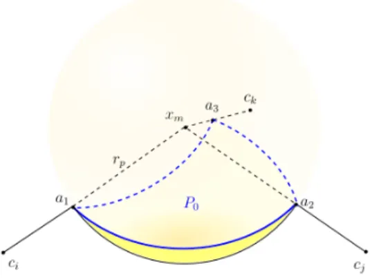
Figure 11: This is the schematic of the concave spherical triangle P0corresponding to an intersection point xm, with the boundary composed of three circular arcs in blue (a¯1a2, a¯2a3anda¯3a1) on the spherical probe. This spherical triangle touches at the same time three VdW-balls at vertices (a1, a2, a3).
We now investigate the different types of singularities that can appear on each of the three patch types. From the definitions of different SES patches, it is relatively easy to calculate the convex spherical patches and the toroidal patches given the
components of the SAS. In the following, we illustrate how to calculate P− exactly,
which provides therefore a complete characterization of the SES-singularities later.
Denote by P0 the concave spherical triangle (P− ⊂ P0) corresponding to an SAS
intersection point xm showed in Figure 11 and by K the set of all intersection points
in I with distances less than 2rp to xm, that is,
K = {x ∈ I : kx − xmk < 2rp, x 6= xm},
so that K collects all SAS intersection points ”near” xm. According to the definition
of P− corresponding to xm and the equation (4.17), we have the following formula:
P− = P0∩ R(xm) = P0∩ T ∩ {p : kp − xmk ≤ kp − xk, ∀x 6= xm, x ∈ I}. (5.24)
The above formula can be used to calculate P− directly, in which R(xm) is a
polyhe-dron. However, this formula is not convenient to calculate, since one has to calculate
T as well as the union of P0 and R(xm). This motivates us to look deep into the
relationship between P− and P0. In the following theorem, we will present a simpler
formula of P−, which allows us to calculate it analytically and more efficiently.
Theorem 5.1. P−=P0\Sx∈KBrp(x) where Brp(x) denotes the open ball (or disc in
The proof of Theorem 5.1 is given in the Appendix. From the definition of
P−, it is not surprising to have the inclusion P− ⊂ P0\Sx∈KBrp(x). However, the
above theorem gives a stronger result that P− and P0\Sx∈KBrp(x) are identical.
This means that the concave spherical patch can be obtained from P0 by removing
the parts intersecting other ”nearby” spherical probes centered at SAS intersection points. This theorem also allows us to characterize the singular circular arcs on
the concave spherical patch P−. We propose a theorem of the SES-singularities as
following.
Theorem 5.2. The following statements hold
[1] There can not exist any singularity on a convex spherical SES patch P+.
[2] On a toroidal patch Pt, two point-singularities occur when the corresponding
SAS circular arc has a radius smaller than rp and they can be computed
fol-lowing the sketch in Figure 13.
[3] On a concave spherical SES patch P−, singular arcs occur when P− does not
coincide with the corresponding concave spherical triangle P0. Further, these
singular arcs form the boundary of P− that does not belong to the boundary of
P0.
Proof. First, if xses is a point on a convex spherical SES patch, then it has a closest
point xsas on an spherical SAS patch. Moreover, xsas is the unique closest point to
xsesfrom Theorem 4.1. This, in turn, implies by Corollary 5.1 that xsescan not be a
singularity. In consequence, there can not exist any singularity on a convex spherical
SES patch P+.
Second, if xses is a point on a toroidal SES patch, then it has a closest point xsas
on an SAS circular arc lm associated with two SAS-spheres Si and Sj. Moreover, xsas
is not unique if and only if xses belongs to [ci, cj] by Theorem 4.2, which happens
only when the radius of lm is smaller than rp and xses is one of two cusps on the
toroidal SES patch as showed in Figure 13. By Corollary 5.1, two point-singularities
on the toroidal patch Ptcan only occur when the corresponding SAS circular arc has
a radius smaller than rp.
Third, if xsesis a point on a concave spherical SES patch P− corresponding to an
SAS intersection point xm, then xsas = xm is a closest point to xses. If xsesbelongs to
the boundary of P−but not to the boundary of P0, then by the formula characterizing
P− in Theorem 5.1 we know that xses lies on another nearby probe ∂Brp(x) where
x ∈ K (and thus x 6= xm). In consequence, x is another closest point to xsesimplying
that xses is singularity by Corollary 4.1. On the other hand, if xses ∈ P− but does
not belong to S
the unique closest point among all SAS intersection points. Assume by contradiction
that there exist another closest point x to xseson some SAS spherical patch Pm. Since
now by Theorem 4.1 the closest point to any point on (ci, x] on the SAS is unique,
this implies that xses = ci (because xm is another closest point). This is however a
contradiction since xsescan not coincide with the center of any SAS-sphere as all the
VdW-radii are assumed to be positive. Further, assume by contradiction that there
exist a closest point x to xses on some SAS circular arc lm. Consequently, xseslies on
the corresponding toroidal patch. According to Theorem 4.2, xses belongs to [ci, cj].
If rp < rlm, then xsescan not belong to the SES which is a contradiction. If rp ≥ rlm,
then xses has to be one of the two cusps. In this case, the two ending points of lm
are both closest points to xses which are also SAS intersection points. This conflicts
with the fact that xsas = xm is the unique closest point among all SAS intersection
points.
Remark 5.1. In the third case of Theorem 5.2, P− can be calculated according
to Theorem 5.1. It is obvious that P− does not coincide with P0 if and only if
P0T
ÄS
x∈KBrp(x)
ä
is nonempty.
Finally, we state a corollary about classifying all points on the SES into four classes according to the number of its closest points on the SAS.
Corollary 5.2. For any point xses ∈ SES, assume that the number of its closest
points on the SAS is N (denoting N = ∞ for an infinite number of closest points). Then, there exists four cases:
[1] N = 1: xses is not a singularity on the SES, and xses has an unique closest
point {x1
sas} on the SAS.
[2] 2 ≤ N < ∞: xses is a singularity on a concave spherical SES patch, and its
closest points {x1
sas, . . . , xNsas} are among the SAS intersection points.
[3] N = ∞: xses is a singularity on a toroidal patch corresponding to an SAS
circular arc (or a complete circle) on which any point is a closest point on the SAS.
5.3. SES-Area and SES-Volume
With the new Voronoi-type diagram as well as the above singularity analysis we can calculate the SES-area and the SES-volume analytically, which shall be explained in the following.
a.. SES-Area
In Connolly’s paper [7], the presence of singularities on the SES concave spherical patches made it infeasible to calculate the SES-area exactly. The characterization of the singularities carried out earlier in this paper allows us to calculate the area of each SES patch and sum them up to obtain the exact area of the whole SES. To
calculate the area of a convex spherical patch P+, we use a similar Gauss-Bonnet
formula as (4.19): X v αv+ X e ke|e| + 1 r2iAP+ = 2πχ, (5.25)
where αv denotes the angle at a vertex v between neighboring circular arcs on the
boundary of P+, ke the geodesic curvature of an edge e on the boundary of P+, AP+
is the area of P+ and χ is the Euler characteristic of P+.
To calculate the area of a toroidal patch Pt analytically, we consider two cases,
and suppose that Pt corresponds to an SAS circular arc lm with radius rlm. In the
case where rlm > rp, there will be no singularity on Pt. With the notations introduced
in Figure 12, we therefore have the following formula for calculating the area of Pt:
APt = rpβm[rlm(θ1+ θ2) − rp(sin θ1+ sin θ2)] . (5.26)
In the case where rlm ≤ rp, there are two singular points on Pt. With the notations
introduced in Figure 13, we have the following formula for calculating the area of Pt:
APt = rpβm[rlm(θ1+ θ2− 2θ0) − rp(sin θ1+ sin θ2− 2 sin θ0)] . (5.27)
To calculate analytically the area of a concave spherical patch P−, we use the
Gauss-Bonnet theorem on the spherical probe again, see Figure 14. In the previous
section, we have obtained that P−=P0\Sx∈KBrp(x), which implies that all
informa-tion about the boundary of P− is known. It allows us to apply the Gauss-Bonnet
theorem on the spherical probe, to obtain:
X v αv+ X e ke|e| + 1 r2 p AP− = 2πχ, (5.28)
where αv denotes the angle at a vertex v on the boundary of P−, ke the geodesic
curvature of an edge e on the boundary of P−, AP+ is the area of P− and χ is the
Euler characteristic of P−.
In summary, the area of each SES patch can be calculated independently and
Figure 12: The yellow patch is a toroidal patch Pton the SES corresponding to an SAS circular arc lm with the radius rlm > rp and the radian βm. θ1 denotes the angle between the line connecting
ci with a point on lmand the disc where lm lies. Similarly, θ2 denotes the angle between the line connecting cj with the same point on lmand the disc where lm lies.
Figure 13: The two yellow parts form a toroidal patch Pt on the SES corresponding to an SAS circular arc lm with the radius rlm < rp and the radian βm. θ0denotes the angle between the line
connecting a singularity on Ptwith a point on lmand the disc where lmlies and θ1, θ2 are defined as in Fig. 12.
b.. SES-Volume
According to the new Voronoi-type diagram, we can calculate the exact SES-volume. We propose to subtract the volume of the region between the SAS and the SES from the SAS-volume to obtain the SES-volume. This region that needs to be
subtracted and which is denoted by Rs can be characterized as below
Rs = {p : −rp ≤ fsas(p) ≤ 0}.
From the new Voronoi-type diagram, we decompose Rs into small regions, each of
which corresponds to a spherical patch Pm, a circular arc lm or an intersection point
xm: Rs∩ R(Pm), Rs∩ R(lm) and Rs∩ R(xm). The volume of the region Rs∩ R(Pm)
is given by VRs∩R(Pm) = 1 3APm(ri+ rp) Ç 1 − r 3 i (ri+ rp)3 å , (5.29)
where APm is the area of the SAS spherical patch Pm, ri+ rp is the radius of the
corresponding SAS-sphere Si on which Pm lies. For Rs∩ R(lm), denote by rlm the
radius of lm and by βm the radian of lm. In the case where rlm > rp, using the
notations of Figure 12, the volume of the region RsTR(lm) is given by
VRs∩R(lm) = βmr 2 p ïr lm 2 (θ1+ θ2) − rp 3(sin θ1+ sin θ2) ò . (5.30)
In the case where rlm ≤ rp, using the notations of Figure 13, it is given by
VRs∩R(lm) = βmr 2 p ïr lm 2 (θ1+ θ2− 2θ0) − rp
3(sin θ1+ sin θ2− 2 sin θ0)
ò +1 3βmr 2 lm q r2 p− rl2m. (5.31)
Consider now Rs∩ R(xm) corresponding to a concave spherical patch P−. Notice
that there might be some flat regions on the boundary of Rs ∩ R(xm), caused by
the intersection of the probe Brp(xm) and its nearby probes, see Figure 14 (right).
Denote by Di the i-th flat region with the boundary composed of line segments and
circular arcs. Furthermore, denote by di the distance from xm to the plane where Di
lies, and by ADi the area of Di. Then, the volume of the region Rs∩ R(xm) can be
formulated as: VRs∩R(xm) = 1 3AP−rp+ X i 1 3ADidi, (5.32)
where, AP−is the area of the concave spherical SES patch P−. Finally, by summing up
the volume of each subtracted region, we obtain the subtracted volume as following: VRs =
X
ξ=Pm, lm, xm
VRs∩R(ξ). (5.33)
Figure 14: On the left, the concave spherical triangle P0 with vertices (a1, a2, a3) corresponds to an intersection point xm. In the case where P− coincide with P0, there will be no singularity on the concave spherical patch. On the right, the concave spherical patch P− does not coincide with P0 and there are singular circular arcs as parts of its boundary. The vertices of P− are (a1, a2, a3, a4, b1, b2, a5). The two flat grey regions D1and D2are formed by the intersection of P0 with two other nearby spherical probes. These two regions have the boundaries composed of line segments and circular arcs.
6. Construction of Molecular Surfaces
In the above sections, we have defined and analyzed the cSAS and the eSAS, as well as the cSES and the eSES. However, all work is based on the explicit knowledge of the components of these molecular surfaces. In this section, we will present a method of constructing the cSAS and the eSAS using a binary tree to construct its spherical patches. After that, we will give a brief construction strategy of the cSES and eSES based on the construction of the cSAS and the eSAS. The construction of molecular surfaces ensures that our previous analysis is feasible.
6.1. Construction of the cSAS and the eSAS
To start the construction, we need some quantities for representing different com-ponents of the SAS. First, an intersection point will be represented by its coordinate
in R3 and an identifier. Second, to represent a circular arc, we use its starting and
ending intersection points (resp. the identifiers), its radius, center and radian as well as an identifier. Finally, to represent a spherical patch, we use the SAS-sphere on which it lies on and the identifiers of all circular arcs forming its boundary. Then, we propose to construct the SAS in five basic steps as below:
2) Calculate each SAS circular arc or circle lmassociated with some Siand Sj. For
each SAS circular arc or circle, we record the information, including the center, the radius, the radian, the corresponding two SAS spheres, the identifiers of the starting and ending intersection points. Notice that each circular arc connects two intersection points.
3) Construct all loops on each SAS sphere Si, which also form the boundaries of
SAS spherical patches on Si. Notice that each loop is composed of circular
arcs, or a complete circle. We start from a circular arc on Si, find another arc
connecting this arc, add it into the loop, and repeat this until we finally obtain
a complete loop. The k-th loop on the i-th SAS sphere is denoted by Li
k.
4) Construct all spherical patches on each SAS sphere Si. Since the boundary
of a spherical patch on Si is composed by one or several loops on Si, we can
use the identifiers of these loops to represent a spherical patch. Denote by Pi
k
the k-th spherical patch on Si. The difficulty lies on determining whether two
loops on Si belong to the boundary of a common spherical patch or not. This
final question will be discussed in the next section.
5) Finally, we should distinguish the cSAS and the eSAS. The cSAS is just the set of all above-constructed SAS spherical patches. To construct the eSAS, we
say that two spherical patches Pki and Plj are neighbors if they have a common
circular arc or circle on their boundaries. Then, we start our construction of the
eSAS, by mapping a faraway point p∞ onto an SAS spherical patch, which is
the initial patch on the eSAS. Then, we add the neighboring spherical patches into the eSAS one by one, to finally obtain the whole eSAS.
6.2. Binary Tree to Construct Spherical Patches
In the above construction process, there remains a problem of classifying the loops on an SAS-sphere into several parts, such that each part forms the boundary of a spherical patch. To do this, we need to determine whether two loops on the SAS-sphere belong to the boundary of a same spherical patch or not. Note that two different loops won’t cross each other but can have common vertices. We propose to construct a binary tree whose leaves are the different spherical patches.
Given a loop L on a fixed SAS-sphere Si, L divides the sphere into two open
parts and it is composed of circular arcs formed by the intersection of Si and other
SAS-spheres. We call the open part of Si which is not hidden by those other
SAS-spheres as the interior of L, denoted by L◦, while the other open part as the exterior
of L, denoted by Lc. We say that another loop L0 on Si is inside L if L0 ∈ L◦, where
L◦ = L ∪ L◦ is the closed hull of L◦ on S
i. Notice that each loop L being part of
Figure 15: On the left is is a brief schematic of an SAS-sphere and the loops on it. There are six loops on the SAS-sphere {L1, L2, L3, L5, L6, L6}, and three spherical patches with the boundaries formed by two loops in green {L4, L5}, three loops in red {L1, L3, L6} and one loop (circle) in blue {L2} respectively. The tree on the right illustrates the corresponding binary tree whose leaves identify the boundaries of three different spherical patches.
boundary of the same patch. By testing if a loop L0 on Si is inside the loop L, we
can classify all loops on Si into two parts: the loops inside L (including L itself)
and the remaining loops outside L. We do this division repeatedly until each loop is tested which results in a binary tree.
To better understand this process, let’s see the example of Figure 15. On an SAS-sphere Si, there are six loops {L1, L2, L3, L5, L6, L6} forming three spherical patches
{P1, P2, P3} with green, red and blue boundaries. The leaves of the binary tree in
Figure 15 represent the boundary of the three spherical patches. To construct the tree, consider all loops {L1, L2, L3, L5, L6, L6} and test with L1, to divide into the
set of loops inside L1 ({L1, L2, L3, L6}) and the set of the remaining loops outside L
({L4, L5}). Then, we test with L2, to find that L2 is inside itself, while {L1, L3, L6}
are outside, which implies that L2 itself forms the boundary of a spherical patch.
Afterwards, we find that {L1, L6} are both inside L3 by testing with L3 and that
{L1, L3} are inside L6 by testing with L6. This implies that {L1, L3, L6} form the
boundary of the second spherical patch, as these three loops are inside each other.
Finally, we test respectively with L4 and L5 to find that they are inside each other
and they form the boundary of the last spherical patch. 6.3. Interior of a Loop
Let L0 and L be two loops on Si. It is left to explain how to test whether L0 is
inside L or not. We assume that L is composed by n circular arcs which are formed by the intersection of Si and other SAS-spheres S10, . . . , Sn0. Denote all intersection
circles by C1, . . . , Cn, where Cj = Si∩ Sj0. The corresponding SAS-balls to S 0
1, . . . , S 0 n
are denoted by B10, . . . , B0n. Since L0 and L do not cross each other, we can determine
if the loop L0 is inside L or not by testing whether a particular point x ∈ L0 is inside
L or not. We denote by xk (1 ≤ k ≤ n) the closest point on Ck to x, which can be
analytically given. Notice that xk has the smallest Euclidean distance in R3 from x
to any point on Ck, which is equivalent to that the shortest path on Si from x to
Ck which ends at xk. For all circles Ck, k = 1, . . . , n, we can then find the circle Ck0
with the minimum path length on Si from x to Ck. The closest point on Ck0 to x is
thus denoted by xk0. With these notations, the following lemma is proposed to test
whether x is inside L or not, note that L0∩Sn
j=1B 0 j = ∅.
Lemma 6.1. Given an arbitrary point x ∈ Si\Snj=1Bj, x is inside L if and only if
xk0 ∈ L.
Proof. We first prove the sufficiency. Assume that x is inside L, i.e. x ∈ L◦ =
L◦∪ L. Assume by contradiction that x
k0 ∈ Ck0 does not belong to L. Then, since
Ck0 ⊂ L ∪ L
c it follows that x
k0 ∈ L
c. Then, the shortest path on S
i from x ∈ L◦
to xk0 ∈ L
c must cross L. In consequence, the intersection point between L and
the shortest path on Si has a smaller path length to x than xk0 does, which is a
contradiction. Therefore there holds that xk0 ∈ L.
Second, we prove the necessity. Assume that xk0 ∈ L. By contradiction again,
we assume that x is not inside L, i.e. x ∈ Lc, which yields that x ∈ Ω := Lc\Sn
j=1Bj
from the lemma’s condition. Then, the shortest path on Si between x ∈ Ω and
xk0 ∈ Ω must cross Γ = ∂Ω. In consequence, the intersection point between Γ and/
the shortest path on Si has a smaller path length to x than xk0 does, which is a
contradiction. Therefore, x lies inside L. 6.4. Construction of the cSES and the eSES
After the construction of the cSAS and the eSAS, patches of the cSES and the eSES can consequently be distinguished since each patch corresponds to one compo-nent of the SAS. An SES patch belongs to the cSES if and only if its corresponding SAS patch belongs to the cSAS. In analogy, an SES patch belongs to the eSES if and only if its corresponding SAS patch belongs to the eSAS.
To construct the whole SES, one can construct each SES patch one by one. A
convex spherical patch P+ on the SES can be obtained directly by shrinking its
corresponding SAS-patch Pm from the SAS-sphere to the VdW-sphere. A toroidal
patch Pt corresponding to an SAS circular arc lmcan also be computed without
Asas(˚A 2 ) Vsas(˚A 3 ) Ases(˚A 2 ) Vses(˚A 3 ) Closed form 1.025416e+02 9.200259e+01 3.223514e+01 1.475567e+01 Proposed method 1.025416e+02 9.200259e+01 3.223514e+01 1.475567e+01 Difference 0 -2.842171e-14 7.105427e-15 -3.552714e-15
Table 1: Surface areas and cavity volumes for a two intersecting atomic system obtained respectively from the closed form expression and the proposed method in the paper. The last row records the difference between these two results.
respectively in Figure 12 and Figure 13 (see also [7]). To calculate a concave
spher-ical patch corresponding to an SAS intersection point xm, we can use the formula
presented in Theorem 5.1:
P−= P0\
[
x∈K
Brp(x),
which is one of the main results of this paper. Notice that P− lies on the spherical
probe centered at xm and its boundary is constituted by circular arcs, which can
be computed analytically. To construct P−, we can consequently use the same
tree-structure (see also Figure 15 on the right) as was used in the previous subsection for constructing SAS spherical patches to classify loops into different sets on the spherical probe (instead of on an SAS-sphere). Some illustrations of the construction of the SESs are provided in the next section (see for instance Figure 20 – 21).
7. Numerical results
In this section, we illustrate some numerical results with the proposed method based on the previous theoretical results.
7.1. A two atomic system
The proposed method gives the analytic expression of surface areas and cavity volumes for both the SAS and the SES if round-off errors are neglected. Here, we test the simplest case of a two atomic system for the comparison of molecular areas and volumes between the closed form expressions based on the properties of a spherical cap (see website [23]) and the proposed method that relies on the Gauss-Bonnet theorem.
With Matlab, we compare the closed form expressions of the surface areas and cavity volumes with the proposed method. We considered two hydrogen atoms
(hav-ing radius 1.2˚A) with distance 2˚A and the probe radius is also set to 1.2˚A. Table 1
reports the molecular areas and molecular volumes obtained. We confirm that the result coincides up to a small error due to round-off errors.
Name Acses Aeses ∆AAesesses Acsas Aesas ∆AAesassas 1ETN 956.636 956.636 0 1397.664 1397.664 0 1B17 3372.577 3372.577 0 4297.098 4297.098 0 101M 7335.438 7096.387 -0.034 8424.749 8413.275 -0.001 3WPE 28575.829 27390.001 -0.043 29747.737 29644.146 -0.003 1A0C 61006.132 54231.268 -0.125 53107.185 51933.798 -0.023 Name Vcses Veses ∆VV ses
eses Vcsas Vesas
∆Vsas Vesas 1ETN 1567.728 1567.728 0 3333.077 3333.077 0 1B17 8630.389 8630.389 0 14435.224 14435.224 0 101M 25029.270 25195.072 0.007 36942.276 36943.700 0.000 3WPE 98651.803 99642.385 0.001 143181.258 143201.169 0.000 1A0C 238282.734 244765.065 0.026 326348.079 326601.929 0.001
Table 2: Different molecular areas (in ˚A2, top) and volumes (in ˚A3, bottom) for five molecules (1ETN, 1B17, 101M, 3WPE, 1A0C from the protein data bank http://www.rcsb.org/pdb/home/ home.do) where we use the notations ∆Ases = Aeses− Acses and ∆Asas = Aesas− Acsas resp. ∆Vses= Veses− Vcses and ∆Vsas= Vesas− Vcsas. The probe radius rp is fixed to be 1.5˚A.
7.2. Molecular areas and volumes
The complete and exterior surface of a molecule can have different areas and volumes. Table 2 reports the surface areas and cavity volumes of different molecules and also the relative errors between the complete results and the exterior results. We observe that the relative difference between the complete and exterior SES-area and SES-volume is up to 12.5% resp. 2.7% in this test cases.
7.3. Comparison with the MSMS-algorithm
We have run the MSMS-algorithm to compare it with the proposed method. It has been observed that if there is no SES-singularity, the exterior molecular areas and volumes from the MSMS coincides with the results of the exterior molecular surface from the proposed method in general. However, in the case where SES-singularities occur on concave spherical patches (which is often the case for complex molecules), the MSMS might fail to give the right SES-area (or SES-volume) due to an incomplete characterization of all SES-singularities.
This can be illustrated on a simple three atomic system where we calculate the molecular areas respectively obtained from the MSMS and the proposed method.
Consider that there are three atoms with the same radius 1.2˚A. In the case of a
probe radius of rp = 2˚A (see Figure 16), there is no SES-singularity and the molecular
areas obtained from the two methods coincide (see Table 3). In the case of a probe
radius of rp = 1˚A (see the left of Figure 17), there is a singular circle on the concave
![Figure 5: Illustration when the point x sas lies on an SAS spherical patch P m which is part of an SAS-sphere S i , and p lies on the segment [c i , x sas ]](https://thumb-eu.123doks.com/thumbv2/123doknet/15016065.681187/12.918.355.564.147.291/figure-illustration-point-lies-spherical-patch-sphere-segment.webp)