HAL Id: hal-03208038
https://hal.archives-ouvertes.fr/hal-03208038
Submitted on 28 Apr 2021HAL is a multi-disciplinary open access
archive for the deposit and dissemination of sci-entific research documents, whether they are pub-lished or not. The documents may come from teaching and research institutions in France or abroad, or from public or private research centers.
L’archive ouverte pluridisciplinaire HAL, est destinée au dépôt et à la diffusion de documents scientifiques de niveau recherche, publiés ou non, émanant des établissements d’enseignement et de recherche français ou étrangers, des laboratoires publics ou privés.
Comparing physical mechanisms for membrane
curvature-driven sorting of BAR-domain proteins
Feng-Ching Tsai, Mijo Simunovic, Benoit Sorre, Aurélie Bertin, John Manzi,
Andrew Callan-Jones, Patricia Bassereau
To cite this version:
Feng-Ching Tsai, Mijo Simunovic, Benoit Sorre, Aurélie Bertin, John Manzi, et al.. Comparing physical mechanisms for membrane curvature-driven sorting of BAR-domain proteins. Soft Matter, Royal Society of Chemistry, 2021, 17 (16), pp.4254-4265. �10.1039/d0sm01573c�. �hal-03208038�
C
omparing
P
hysical
M
echanisms
for
M
embrane
C
urvature-
D
riven
S
orting
of
B
AR-
D
omain
P
roteins
Feng-Ching Tsai1*, Mijo Simunovic2,3,#, Benoit Sorre1,4#, Aurélie Bertin1, John Manzi1, Andrew
Callan-Jones4*, Patricia Bassereau1*
1- Institut Curie, Université PSL, CNRS UMR168, Sorbonne Université, Laboratoire Physico Chimie Curie, 75005 Paris, France
2- Department of Chemical Engineering, Columbia University, New York, NY 10027, USA 3- Department of Genetics and Development, Columbia Stem Cell Initiative, Columbia
University Irving Medical Center, NY 10032, USA
4- Laboratoire Matière et Systèmes Complexes, UMR 7057 CNRS, Université de Paris, Paris, France.
# these authors contribute equally * corresponding authors
Abstract
Protein enrichment at specific membrane locations in cells is crucial for many cellular functions. It is well-recognized that the ability of the proteins to sense membrane curvature contributes partly to their enrichment in highly curved cellular membranes. In the past, different theoretical models have been developed to reveal the physical mechanisms underlying curvature-driven protein sorting. This review aims to provide a detailed discussion of the two continuous models that are based on the Helfrich elasticity energy, (1) the spontaneous curvature model and (2) the curvature mismatch model. These two models are commonly applied to describe experimental observations of protein sorting. We discuss how they can be used to explain the curvature-induced sorting data of two BAR proteins, amphiphysin and centaurin. We further discuss how membrane rigidity, consequently the membrane curvature generated by BAR proteins, could influence protein organization on the curved membranes. Finally, we address future directions in extending these models to describe some cellular phenomena involving protein sorting.
1. Introduction
The basic structure of cellular membranes is a sheet-like, 3-5 nm thick lipid bilayer formed by self-assembled amphipathic phospholipids 1. In cells, a large amount of proteins are bound on
or embedded in the membranes. Many cellular functions depend on the ability of cells to robustly and dynamically reshape cellular membranes 2. A prominent example is the generation of transport
vesicles in endocytosis and intracellular trafficking that allow cells to intake and transport cargos among different organelles. During these processes, cellular membranes undergo significant shape change, resulting in the generation of high membrane curvature. For instance, in clathrin-mediated endocytosis, the plasma membrane is deformed into vesicular buds with a diameter of 50-200 nm; and the buds are connected to the donor membrane via a thin neck, with a width of 25-150 nm and variable length, either very short and catenoid-like, or longer, on the order of 100 nm 3. Emerging
evidence has shown that lipids and membrane proteins both contribute substantially to the generation of cellular membrane curvature. Conversely, membrane curvature can influence how lipids are distributed, and how proteins bind and assemble on membranes. Over the past decades, several mechanisms of membrane curvature generation have been revealed (please refer to other reviews 4-11. In this review, we focus our discussion on curvature-dependent protein
distribution/sorting. For curvature-dependent lipid distribution/sorting, readers are referred to other reviews 6, 12, 13.
Lipid bilayers are complex soft matter systems with fluid in-plane and elastic out-of-plane behaviors. Within the bilayer, lipids and proteins can diffuse freely; thus, the bilayer is fluidic-like
14-16. Considering the bilayer as a whole, it behaves as a continuous elastic sheet that can be bent
and resists to stretching limited to a few percent of its area. Based on the fluid mosaic model described by Singer and Nicolson, and the framework established by Helfrich and many others, continuous physical descriptions of lipid bilayers based on curvature elasticity have quantitatively explained large-scale behaviors of membrane at equilibrium 17-22. Their work has provided the
basic foundation for interpreting experimental observations 6, 10, 23-28. The so-called Helfrich
curvature-elasticity energy relates the free energy of a lipid bilayer to its curvature and tension 18,
𝐹 = 1
2𝜅(𝑐 + 𝑐 − 𝑐 ) + 𝜅 𝑐 𝑐 + 𝜎 𝑑𝐴
(1) where 𝐴 is the total membrane area. It is constructed based on the two principal curvatures of the bilayer, 𝑐 and 𝑐 , the spontaneous curvature of the bilayer 𝑐 , together with two elastic coefficients: the bending modulus and the elastic modulus of the Gaussian curvature, 𝜅 and 𝜅 , respectively, and the membrane tension 𝜎. The bending modulus and the modulus of the Gaussian curvature of a typical bilayer is around 20 k T and 50 k T, respectively 29, 30. Membrane curvature
is characterized by its absolute value as well as its sign, which requires to distinguish the two sides of the membrane surface 5. Different conventions can be chosen for the curvature sign. In keeping
with BAR domain literature, we define the sign of membrane curvature to be positive when the membrane curves toward the bound protein and negative when it bends away (Fig. 1). Importantly, if an asymmetry of the two leaflets exists, which could result from different lipid numbers or compositions, from different bulk compositions on each side of the bilayer, and from protein binding or inserting into the leaflets in an asymmetric fashion, the bilayer spontaneously bends towards one direction. To account for this phenomenon, a phenomenological term called "spontaneous curvature" 𝑐 was introduced to describe that, in the absence of external stresses, i.e.
in the relaxed state, the membrane is “spontaneously” curved. When first introduced by Helfrich, it was assumed that the asymmetry of the membranes is due to different lipid compositions in the two constituent monolayers or due to different aqueous environments of the two monolayers 22. It
has to be noted that the Equation (1) is valid only when 1/𝑐 is much larger than the thickness of the bilayer 𝑑. In the case where |𝑐 |𝑑 ≥ 1, the Helfrich curvature-elastic energy expression has to include higher order terms 31. The spontaneous curvature is related to the residual torque in a flat
membrane, and the cross term -𝜅 𝐶𝑐 , where 𝐶 = 𝑐 + 𝑐 , is the work done against this torque in going from the flat reference state to a state with curvature C. Note that this term reflects broken up-down symmetry in the bilayer 32. It is important to note that the spontaneous curvature 𝑐 is
different from the intrinsic curvature 𝑐 , which is a geometrical parameter describing the shape of a relaxed membrane32. Also, for a pure lipid membrane, i.e. in the absence of proteins, any
inhomogeneity in the spontaneous curvature, for instance due to local in-plane density differences of the lipids, should relax quickly because the two constituent monolayers are free to slide over each other. Thus, for a pure lipid membrane, 𝑐 is constant over the entire membrane 22. To account
for the presence of membrane proteins, several models based on the Helfrich curvature-elastic theory have been developed 5, 11, 33. These models aim to explain how the local concentrations of
proteins are coupled to and can influence the curvature and the stiffness of the membrane, and conversely how membrane curvature can influence protein localization, meaning proteins have a preferred affinity to be on membranes with a specific curvature. This phenomenon when proteins bind to curved membranes at a higher affinity than to flat membranes is called “curvature-induced protein sorting”.
Figure 1. Schematics of positive and negative membrane curvature.
In cells, a plethora of membrane proteins have been identified as being capable of reshaping cellular membranes 4-6, 9, 13, 34, 35. Here, we focus our discussion on the proteins from the
Bin-Amphiphysin-Rvs167 (BAR) domain superfamily 36, 37. BAR domains form antiparallel
homodimers that are intrinsically curved and have anisotropic crescent shapes. Based on their crystal structures, BAR domains can be classified into three major subfamilies: the classical BAR, the longer and less curved Fes/CIP4 homology-BAR (F-BAR) and the inverse-BAR (I-BAR) domains. Some classical BAR domains contain an N-terminal amphipathic helix, named N-BAR domains. The most prominent function of BAR domain is its ability to sense and generate membrane curvature, which have significant impact on their biological functions 37-41. The
I-BAR domain interacts with membranes via its convex surface. Indeed, it has been shown that the classical BAR domains prefer to associate with membranes with a positive curvature 42-45, while
I-BAR domain prefers to bind to membranes with a negative curvature 46. Emerging cell biology
studies have shown that the curvature sensing ability of BAR proteins contributes to their cellular localization and consequently their cellular functions 47-50. To reveal physical mechanisms by
which BAR proteins sense membrane curvature, computer simulations, theoretical modeling and in vitro reconstitution systems have been developed 6, 10, 50. These studies have revealed parameters
that determine how BAR proteins bind on membranes, and concomitantly their curvature sensing activities. For instance, BAR-membrane interactions depend not only on the structures of the proteins, but also on membrane shape and tension, as well as protein densities on the membranes
10, 51.
In this review article, we begin by describing two continuous models based on the Helfrich free-energy for describing curvature-dependent protein sorting, (1) the spontaneous curvature model and (2) the curvature mismatch model. We then focus our discussion on one of the in vitro experimental approaches, membrane nanotube pulling, designed to assess curvature-dependent protein sorting. We further revisit experimental data of BAR protein amphiphysin and centaurin, and we discuss how the current models deepen our knowledge on their curvature sensing. Finally, using cryo-EM, we observed two different organizations of BAR domains on tubes of different radii. We close this review with suggestions for future work.
2. Modified curvature-elastic models of protein-bound membranes
It had been predicted by Helfrich, Leibler, Markin and many others that membrane impurities or proteins can modify the spontaneous curvature of the protein-bound membrane due to the asymmetrical distribution of the peripheral membrane proteins on the two leaflets or the asymmetrical shapes of transmembrane proteins 18, 22, 52, 53. This notion has been demonstrated
experimentally, for instance by membrane nanotube pulling assay as discussed below. To take this effect into account, theoretical models have been proposed based on the Helfrich curvature-elastic theory 43, 44, 46, 54-57.
In the following, we discuss two models that have been widely used to explain experimental results on how proteins modulate membrane elastic energy, and how the membrane association of proteins is affected by membrane curvature. Note that both models below assume a lipid bilayer with a symmetric lipid composition and aqueous environment, and with a single type of proteins binding on the membrane. Also, direct protein-protein interactions are neglected in order to highlight the specific effects of membrane curvature coupling to local protein concentration, which in our theoretical analysis is quantified as the protein areal density (in proteins/𝜇𝑚 ), or alternatively as the areal fraction (in %).
2.1. Spontaneous curvature model
The spontaneous curvature model was originally introduced to describe the coupling between curvature and asymmetry of the membrane due to constituents’ shapes or unequal
distribution of constituents across the bilayer 6, 52, 53, 58. It was next implemented to describe the
membrane curvature-dependent sorting of BAR protein amphiphysin 43 and membrane reshaping
by lipopolysaccharide 59. In the simplest form of this model, it is assumed that the protein-induced
spontaneous curvature is coupled to the local protein concentration. Notably, it is assumed that the proteins do not necessarily influence the bending rigidity of the membrane. The general expression of the elastic energy of the system can be written as
𝐹 = 1 2𝜅(𝐶 − 𝐶 (𝜙)) 𝑑𝐴 = 1 2𝜅𝐶 − 𝜅𝐶𝐶 𝜙 + 1 2𝜅𝐶 𝜙 𝑑𝐴 (2) where 𝜅 is the bending modulus of the protein-bound membrane, 𝜙 is the protein areal fraction on the membrane (in %), and 𝐶 (𝜙) is the spontaneous curvature of a protein-bound membrane patch that depends on protein areal fraction. The expression in Equation (2) is the leading term in curvature deviations away from the reference state with 𝐶 = 𝐶 (𝜙). One might object to considering a reference state that depends on 𝜙 in cases where it is not uniform on the membrane. We note that one can always write the free energy on a region of uniform curvature and uniform protein density (such as a large membrane reservoir), and then perform a Taylor expansion to obtain the energy on nearby regions with different values of 𝐶 and 𝜙. Spatial non-uniformities could be treated by including gradient-squared contributions in 𝜙, and should only be important when membrane curvature changes abruptly, such as at the GUV-tube neck region in the membrane nanotube pulling assay (see Section 3.1). Because the nanotube pulling experiments usually involve spatial averages over membranes, these regions are not specifically considered. At low protein areal fractions and assuming that the proteins bind to the membrane independently of each other, the spontaneous curvature term is assumed to depend linearly on 𝜙 60. It can be written
as
𝐶 (𝜙) = 𝐶 𝜙 (3)
where 𝐶 is a parameter that reflects the intrinsic curvature of the part of the protein that interacts with the membrane. Thus, 𝐶 does not correspond directly to the shape of the protein; it is determined by the interplay between the protein and the membrane. In this model, the first term 𝜅𝐶 describes the elastic energy of the membrane in the absence of the proteins. Through the second term 𝜅𝐶𝐶 𝜙, the membrane curvature is coupled to the protein area fraction. The third term 𝜅𝐶 𝜙 could be considered as an effective repulsion between the proteins, which is related to the spontaneous tension introduced by R. Lipowsky 27, 54. More general two-body protein-protein
interactions could be included by adding a generic energy term varying like 𝜙 . These terms have been considered by 44, 46, 51, 52.
2.2. Curvature mismatch model
The curvature mismatch model was first developed by Kralj-Iglic et al. to describe the protein distribution coupled to cell shape 61, and later to account for other experimental
observations of curvature-dependent protein sorting in reconstituted systems and in living cells 46, 50, 62. At the molecular scale, protein-membrane binding involves either the deformation of the
of the bound-protein due to the membrane curvature, or a combination of both. According to this model, at low enough protein density (i.e. low areal fraction), such that proteins bind independently of one another, the elastic energy of protein-membrane binding should be proportional to the local protein areal fraction and to the protein-membrane binding energy, which is expected to depend on the local membrane curvature. This binding energy should be maximal for a certain curvature, and the simplest model is to assume that it is proportional to the square of the difference between the mean membrane curvature C and this optimal curvature, which we refer to as 𝐶 . The corresponding elastic energy of the system can be written as 46, 63
𝐹 = 1
2𝜅𝐶 + 1
2𝜅̅𝜙 𝐶 − 𝐶 𝑑𝐴
(4)
where 𝐶 is a phenomenological coefficient related to the protein’s intrinsic curvature, and 𝜅̅ is an elastic constant reflecting the energy penalty for the mismatch of 𝐶 and 𝐶 , thus describing the strength of the curvature mismatch.
We note that for the curvature mismatch model, it is possible to define a reference curvature for a given value. From Equation (4), we can show readily that
𝜅 2𝐶 + 𝜅 2𝜙 (𝐶 − 𝐶̅ ) = 𝜅 + 𝜅̅𝜙 2 𝐶 − 𝜅̅ 𝐶̅ 𝜙 𝜅 + 𝜅̅𝜙 + 𝑔(𝜙) (5)
In the above, g is a function of and the spontaneous curvature is the second term in the squared bracketed term. Of course, this is not in the same form as in the spontaneous curvature model. Implicit in this model is that the curvatures C and 𝐶 are small and that the squared-bracketed term above is also small. The above equation also shows that proteins modify the membrane bending stiffness, in a linear fashion with 𝜙. Compared to the spontaneous curvature model, there is no effective repulsion between the proteins, i.e., a 𝜙 term, which is reasonable for the low protein density regime considered here. Similar to the spontaneous curvature model, the 𝜅̅𝜙𝐶𝐶 term relates the local protein area fraction to membrane curvature. For detailed analysis on the effect of protein anisotropy, readers are referred to the study of S. Svetina 63.
2.3. Other contributions to the free energy of the system: mixing entropy term
Given that the system has two components, the membrane-bound proteins and the lipids, an inhomogeneous distribution of either components is entropically unfavourable. The entropic energy of mixing in the two components system, here the membrane-bound proteins and the lipids, is given by the Flory-Huggins form,
𝐹 = 𝑘 𝑇𝜌[𝜙 ln 𝜙 + (1 − 𝜙) ln(1 − 𝜙)]𝑑𝐴 (6) where 𝑘 is Boltzmann’s constant and 𝜌 is the inverse of the membrane area occupied by the bound protein. This term has been included in the models (see below), but becomes less important when the protein size increases (i.e. 𝜌 decreases).
The above-mentioned models have nevertheless neglected some aspects such as membrane area differences between the leaflets, potentially multiple protein-membrane binding modes, and direct protein-protein interactions, such as protein oligomerization. For instance, Cryo-EM studies have shown that protein-protein interactions among N-BAR domains or F-BAR domains induce highly ordered helical coats of the domains on tubular membranes, resulting from directional protein-protein interactions 64-66. Also, both models assume that membrane-bound proteins are in
an isotropic fluid state, i.e., the proteins can freely diffuse and rotate on the membrane. However, since some proteins have anisotropic shape, at a relatively high protein density on the membrane and facilitated by the enrichment related to curvature coupling, these proteins could undergo an isotropic-nematic phase transition, resulting in ordered organization on the membrane 54.
2.5. Similarities and differences between the two models
The spontaneous curvature model and the curvature mismatch model both couple the membrane curvature 𝐶 and the local protein areal fraction 𝜙 in order to describe how proteins sense and thus consequently preferentially bind to membrane locations with given membrane curvatures. In the spontaneous curvature model, it corresponds to the term (𝜅𝑐 )𝜙𝐶, while in the curvature mismatch model to 𝜅 𝑐 𝜙𝐶. Notably, a similar term, Λ𝜙𝐶, was introduced by Leibler with a coupling parameter Λ 53. Also, in both models, information considering the organization of
proteins on curved membranes is not required.
In the spontaneous curvature model as written, we have not considered an explicit dependence of the membrane bending rigidity 𝜅 on protein density. In the simplest model, including this dependence would add a term varying as 𝜙𝐶 in the free energy. We note that more sophisticated versions of this model have indeed included such a dependence 52, 58. It should be
noted that this 𝜅 is completely different from the renormalized one predicted by Leibler 53, in
which an effective rigidity arises from the 𝜙𝐶 term in the free energy upon integrating over protein concentration degrees of freedom, and thereby writing an effective free energy that depends only on curvature 53, 67. In the curvature mismatch model, bound proteins modify the energy term in 𝐶 ;
this may be interpreted as a protein modification to 𝜅 that is linear in 𝜙. The inclusion, or not, of protein modification to 𝜅 gives rise to different predictions on how proteins enrich on membranes as a function of membrane curvature (namely, protein sorting). The spontaneous curvature model, without a protein effect on 𝜅, predicts a monotonic increase of protein sorting, while the curvature mismatch model yields a non-monotonic protein sorting. Another difference between the two models is that in the spontaneous curvature model, there is an extra term 𝜅(𝐶 𝜙) , which depends on 𝜙 and suggests protein repulsion. A hybrid model can be constructed in which the bending stiffness and spontaneous curvature both depend linearly on 𝜙, as well as having the effective protein repulsive term. This approach has been used to describe the membrane curvature sorting of an integral membrane protein potassium channel KvAP 63, 68.
Interestingly, the curvature mismatch model predicts protein phase separation on curved membranes 46. It originates from the coupling between protein density and membrane curvature,
which is non-linear in 𝜙 in the curvature mismatch model. The curvature mismatch model has been used to predict phase separation of dynamin and of FtsZ on membrane tubes 69, 70.
of Zhu et al., explicit protein-protein interactions were included using van der Waals type model, and these are required to account for phase separation 44. These predictions were confirmed by
experimental data in which phase separation of the IRSp53 I-BAR domain on membrane tubes pulled from giant unilamellar vesicles (GUVs) was observed 46. Such phase separation might play
roles in cellular processes such as endocytosis and filopodial initiation. The strong coupling of protein local density and membrane curvature could give rise to protein-driven membrane deformation as well as clustering of signaling lipids such as PI(4,5)P2 at the membrane deformation
sites that are both essential for the cellular processes 71, 72. Indeed, live cell imaging has revealed
that filopodia formation is often preceded by the formation of a cluster of I-BAR domain protein IRSp53 on the membrane 46, 73.
To the best of our knowledge, there is no definite guideline when determining which model to use for fitting experimental data. The main difference between the spontaneous curvature and curvature mismatch models is that the latter includes a term that varies as 𝜙 𝐶 whereas the former does not. Both models contain a “spontaneous curvature” term ~𝜙 𝐶. The ratio of the two terms is a parameter that sets a curvature scale. If this curvature scale is large compared with the membrane curvature C, then one can argue that the 𝜙 𝐶 term can be ignored, otherwise it cannot. Thus, in the case of (shallow) I-BAR proteins, where the curvature scale is expected to be small, the 𝜙 𝐶 must be included46. In the case of amphiphysin, which contains a BAR backbone and
amphipathic insertions, the curvature scale could be expected to be higher. Therefore, in principle, the spontaneous curvature model can be justified to fit the sorting data of amphiphysin43.
A recent study suggested that if proteins have negligible contributions on membrane stiffness, such as the insertion of amphipathic helices (AH), the spontaneous curvature model may be more appropriate to describe protein-membrane binding, and if proteins form scaffolds on membranes, such as BAR proteins, the curvature mismatch model may be more suitable 57.
However, this assumption may not be valid for all AH insertions. For example, while it was shown that binding and helix insertion of the epsin N-terminal homology (ENTH) domain can soften membranes 74, amphipathic peptides were shown to stiffen the membrane 75. Moreover, in
physiological conditions, AH insertion and scaffolding are usually entangled, such as in the case of N-BAR protein amphiphysin. Obviously, if protein sorting plotted as a function of membrane curvature has a clear peak value (see for instance 46), one should use the curvature mismatch model.
A priori, we expect that proteins of the same family should be described by the same model. Moreover, due to their simplicity, both models neglect some aspects as discussed above. Especially, at high protein density, neither of the models would fully describe the observed phenomena since direct protein-protein interactions are neglected.
In Section 4, we used the spontaneous curvature and curvature mismatch models to fit the sorting data of the full-length amphiphysin, i.e. BAR domain followed by a disordered domain and a SH3 domain. We further performed statistical tests to compare the fitting results of the two models, and we discussed these results in details.
3. Testing these models experimentally 3.1. Membrane nanotube pulling assay
Emerging results obtained by the membrane nanotube pulling approach have demonstrated curvature-controlled protein polymerization, such as for dynamin 76, and protein sorting, such as
for amphipathic lipid packing sensor (ALPS) 77, BAR proteins 42-44, 46, 51, 78-81, and α-synuclein
motifs 6. The nanotube pulling assay has been extensively used for quantitatively assessing
curvature sensing and generation abilities of proteins. In this assay, a small amount of biotinylated lipids (around 0.2 mol%) is incorporated in the GUV membrane to establish its binding to micrometer-size streptavidin-coated beads. A membrane nanotube is generated by first establishing binding between the GUV held by a micropipette on a micromanipulator and the bead trapped with optical tweezers, followed by moving the GUV away from the bead 82. By tuning the
aspiration pressure in the micropipette, one can control the GUV membrane tension, consequently the tube radius (in the absence of proteins, the tube radius 𝑅 = ). The nanotubes have a typical radius ranging from 7 nm to a few hundreds of nanometers, comparable to biologically-relevant membrane curvatures 2. Depending on the proteins of interest and the corresponding signs of
membrane curvature to be assessed, one can either micro-perfuse the proteins adjacent to the membrane nanotube to test protein positive curvature-sensing, or one can encapsulate the proteins inside GUVs prior to pulling tubes to probe negative curvature-sensing. Eventually, the protein enrichment on tubes is quantified by the sorting ratio 𝑆 using fluorescent lipids and proteins, and confocal microscopy: 𝑆 = /
/ is given by the relative fluorescence intensity of the
proteins on the tube (𝐼 ) and on the GUV membrane (𝐼 ), normalized by the relative fluorescence intensity of lipid probes on the tube (𝐼 ) and on the GUV membrane (𝐼 ). One can quite generally measure protein enrichment on the tube as compared with the nearly flat GUV
6. As we discuss below, the sorting ratio depends on the protein density Φ on the GUV and, of
course, on the type of protein. Furthermore, at low values of Φ proteins generally sense tube curvature, but do not significantly alter the tube radius – often referred to as “curvature sensing”. In contrast, at higher densities the protein are both enriched and feedback on the tube curvature – referred to as curvature generation 10.
3.2 Sorting ratios corresponding to the 2 models 3.2.1. Spontaneous curvature model
To describe the sorting data of amphiphysin obtained by the nanotube pulling assay by Sorre et al., the spontaneous curvature model was modified to incorporate the protein mixing entropy and protein–protein interactions 43. For small differences between protein areal fractions
on the tube 𝜙 and on the GUV 𝜙 , after second-order Taylor expansion the free energy can be approximated as 𝐹 = 2𝜋𝑅𝐿 𝜅 2 1 𝑅 − 2𝐶̅ 𝜙 𝑅 + 1 2𝜒Δ𝜙 + 𝜎 − 𝑓𝐿 (7)
where Δ𝜙 = 𝜙 − 𝜙 , 𝜒 =
( )+ 𝜅𝐶 is the effective osmotic susceptibility, f is the pulling
force and L the tube length. In the limit of vanishing protein density on the GUV, 𝜙 ≈ 0, we have 𝜒 ≈ + 𝜅𝐶 . The sorting ratio is given by
𝑆 = 1 +Δ𝜙
𝜙 = 1 + 𝜅𝐶 𝑅𝜒𝜙
(8) In a very dilute situation, for instance where the protein density Φ < 50 μm , or conversely the areal fraction 𝜙 = Φ × < 0.25% (for 𝜌 = 1 50 𝑛𝑚 ), the sorting ratio can be written as
𝑆 = 1 + 𝜅𝐶 𝑘 𝑇𝜌
1 𝑅
(9) In this regime, the sorting ratio increases linearly with 1/𝑅 and is independent of 𝜙 . By fitting experimental sorting data with Equation (9), one can obtain 𝐶 . We note that Equations (8) and (9) can only be applied to low protein density regime. With increasing protein density, the Taylor-expansion of the mixing free energy up to quadratic order becomes less valid. In this case, the entropic part of the effective susceptibility can be neglected. The sorting ratio still depends linearly on the curvature 1/𝑅 but also on 𝜙 :
𝑆 = 1 + 1 𝐶 𝜙
1 𝑅
(10) 3.2.2. Curvature mismatch model
The curvature mismatch model was also modified to include energies related to protein-membrane interaction, protein-protein interaction and protein/lipid mixing entropy 46. The free
energy of the system can be written as
𝐹 = 2𝜋𝑅𝐿 + 𝜙 − 𝐶 + 𝑓 + 𝑓 (11)
where 𝑓 and 𝑓 are the energy densities of membrane stretching and protein mixing entropy on membranes. 𝑓 = 𝑘 𝑛 𝑎 + 𝑛 𝑎 − 1 , where 𝑘 is compression/dilation modulus, 𝑛 is the number of the lipids per unit area, 𝑛 is the number of the membrane bound proteins per unit area, and 𝑎 and 𝑎 are the membrane areas occupied by a membrane bound protein and a lipid, respectively. We note that the membrane tension is related to the stretching energy, that is 𝜎 = 𝑘 1 − 𝑛 𝑎 − 𝑛 𝑎 and the tube pulling force is given by 𝑓 = 2𝜋𝑅 + 𝜎 46.
At equilibrium the chemical potentials of the lipids and proteins on the GUV and on the tube are equal, thus an implicit dependence of 𝜙 on the tube curvature can be written as
𝜙 𝜙 1 − 𝜙 1 − 𝜙 / = exp 𝜅̅𝑎 𝑘 𝑇 𝐶 𝑅 − 1 2𝑅 (12) At low protein density regime, both 𝜙 and 𝜙 ≪ 1, thus the relation between the sorting ratio 𝑆 and the tube curvature 𝐶 = 1/𝑅 is a Gaussian distribution, with a maximum at 𝐶 = 𝐶 as observed e.g. for the I-BAR domain of IRSp53 46.We note that Equation (12) can be applied to different
protein density regimes and predicts that the sorting ratio (𝑆) decreases with increasing protein areal fraction on GUVs (𝜙 ), consistent with the experimental data of Prevost et al. 46. This is
because when the protein density on a GUV increases, the protein density on the corresponding tube ultimately saturates, resulting in a decrease in the (relative) sorting ratio. By fitting experimental sorting data with Equation (12), one can obtain 𝜅̅ and 𝐶 .
4. Comparing the two models on experimental sorting data on two BAR domain proteins 4.1 N-BAR Amphiphysin 1
Here, we have revisited our previous analysis of curvature-induced sorting measurements for human amphiphysin 1 43. Amphiphysin 1 has an N-terminal N-BAR domain, followed by a
central clathrin and AP-2 interacting domain, and finally a C-terminal SH3 domain. The measurements were performed using the nanotube pulling approach where the full length human amphiphysin 1 (labelled with Alexa 488, referred to as amphiphysin hereafter) was injected adjacent to membrane tubes pulled from GUVs 43. The GUVs were composed of DOPC, DOPE,
and DOPS (in 1:1:1 molar ratio). At protein surface densities Φ > 1000 μm it was shown that amphiphysin has a mechanical effect on the membrane, where the tube radius is no longer dependent on the membrane tension but instead is controlled by the amphiphysin scaffold formed on the tube, leading to a 7±2 nm tube radius. At lower densities, Φ < 1000 μm , amphiphysin can sense positive membrane curvature without significantly altering the tube, resulting in the enrichment of amphiphysin on the tubes. To explain the observed curvature sorting of amphiphysin, the spontaneous curvature model (Equation (9)) was used to fit the sorting results at very low protein density ( Φ < 50 𝜇m ), obtaining 1/𝐶 = 0.8 ± 0.4 nm 43. At moderate
density (280 ± 100 μm−2), by using Equation (10), one obtained 1/𝐶 = 1.9 ± 0.4 nm 43. Note
that the values of 1/𝐶 are quite low, far from the scaffold radius, although it is comparable with the predicted value for amphipathic helix insertion in the membranes 60. The large discrepancy
between 1/𝐶 deduced from the sorting experiments and the structural data on amphiphysin BAR domain (see below) or our measurements of the scaffold size was puzzling.
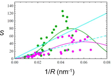
Since the curvature mismatch model should be valid for a large range of protein densities as shown previously in 46, we used it to fit the sorting data of amphiphysin obtained at both low
(𝛷 < 50 𝜇m ) and higher protein densities (𝛷 > 50 𝜇m ). As shown in Fig. 2A, we note that the sorting ratio decreases when the protein density on vesicles increases, as expected 46. For
protein densities 𝛷 < 50 𝜇m and 50 𝜇m < Φ < 120 𝜇m , we obtained 1/𝐶 = 9 nm and 13.5 nm, respectively (green and magenta lines in Fig. 2B, and Table 1). We also fitted these two datasets with the spontaneous curvature model using Equation (9), and we found 1/𝐶 that does not agree with the crystal structure and scaffolding tube radius (cyan lines in Fig. 2B, and Table 1). To compare the fitting results of the two models for these two data sets, we performed an F test and the AIC (Akaike Information Criterion) test. Based on the results of the two tests, the curvature mismatch model gives a better fit to our data than the spontaneous curvature model does (see Table 4 in the Appendix).
We also measured amphiphysin sorting at higher values of Φ , which is shown in Fig. 2C. There are two interesting points to note about these data. First, one readily notes that sorting data correspond to only a narrow range of tube curvatures, centered at around 0.1 nm-1. This shows that
in this protein density regime the proteins modify the tube curvature. Thus, at higher protein densities, both curvature sensing and generation are observed (see also Fig. 4C of 43). Second,
although a significant sorting ratio is measured, the data are noisier and do not reach the same levels as at lower protein densities. Based on these observations, the high protein density data are not amenable to the model fit as presented at lower densities.
Figure 2. Sorting ratio S of amphiphysin as a function of tube curvature 1/R. Green circles 𝛷𝑣 < 50 𝜇𝑚 , Magenta circles, 50 𝜇𝑚 < 𝛷 < 120 𝜇𝑚 , Orange circles 120 𝜇𝑚 < 𝛷 < 500 𝜇𝑚 , and Cyan circles 𝛷 > 500 𝜇𝑚 . In (B), solid green and solid magenta lines are the fits to the corresponding data set using Equation (12) (Curvature mismatch model). Solid cyan and dashed cyan curves are the fits using Equation (9) (Spontaneous curvature model) to data sets of 𝛷 < 50 𝜇𝑚 and 50 𝜇𝑚 < 𝛷 < 120 𝜇𝑚 , respectively. (C) is an enlargement of (A) showing sorting data at 120 𝜇𝑚 < 𝛷 < 500 𝜇𝑚 (orange circles), and 𝛷 > 500 𝜇𝑚 (cyan circles). Note that part of the data is from 43.
Protein density Φ Protein areal fraction 𝜙 𝜅̅ 𝐶 1/𝐶 1/𝐶 Φ < 50 𝜇m 𝜙 < 0.25 % 14.7 ± 1.7 k T 0.111 ± 0.008 nm-1 9.0 nm 1.0 nm
50 𝜇m < Φ < 120 𝜇m 0.25 % < 𝜙 < 0.6 % 26.8 ± 2.2 𝑘 𝑇 0.074 ± 0.003 nm-1 13.5 nm 1.8 nm
Table 1. Fitting parameters for amphiphysin sorting data shown in Fig. 2B using Equation (12) of the curvature mismatch model, 𝜅̅ and 𝐶 , and using Equation (9) of the spontaneous curvature model, 𝐶 . The membrane area occupied by the protein is 50 nm2.
Although one cannot directly compare the 1/𝐶 values obtained from tube pulling experiments either to the crystal structures of N-BAR domain nor to the diameters of the N-BAR domain decorated tubes (which also depends on membrane composition through and 𝜅̅ 46), the
value of 1/𝐶 reflects to a certain extent, how curved the N-BAR domain is. Notably, the obtained 1/𝐶 ≈ 11 nm (averaged by the two 𝐶 values obtained here, as shown in Table 1) is very close to the curvature of the concave surface of the crystal structure of Drosophila amphiphysin N-BAR domain, ~ 1/11 nm 83. Also, it is close to the radius of N-BAR domain deformed membrane tubes
observed by Cryo-EM, ~12.4 nm for Drosophila amphiphysin N-BAR domain 66, and ~11 nm for
human amphiphysin 2 N-BAR domain 84. Another study of Drosophila amphiphysin N-BAR
domain using the tube pulling approach from GUVs reported an effective spontaneous curvature 𝐶 , i.e. 𝐶 (𝜙) in Equation (2), to be around 0.1 nm-1, which is comparable with 1/𝐶 ≈ 11 nm obtained here 42. Eventually, the value is also close to that deduced from our scaffolded tubes. Note
that the scaffold radius measured either by fluorescence or from the tube force corresponds to the mid-plane of the membrane of the tube. To compare with the curvature of the BAR domain obtained by crystallography or electron microscopy, a half-bilayer thickness should be added, resulting in a tube radius of the order of 10-11 nm, and a little bit higher if we consider the protein thickness on the tubes. Notably, the disordered domains of amphiphysin can also influence the tube radius due to steric interactions between the disordered domains 85.
In conclusion, we find that the curvature mismatch model is better suited to model amphiphysin curvature sorting than the spontaneous curvature model.
4.2. 𝛽2 centaurin
Although 𝛽2 centaurin and amphiphysin both contain BAR domains, their structures differ in three main ways. First, the BAR domain of 𝛽2 centaurin has an intrinsic radius of curvature of ~ 40 nm, which is flatter than the BAR domain of amphiphysin (~ 11 nm) 83, 86. Second, the BAR domain
of 𝛽2 centaurin does not contain amphipathic helices unlike amphiphysin. Third, 𝛽2 centaurin contains a pleckstrin homology domain (PH domain) that contributes to the binding of centaurin to membranes 71. Here, we assessed the curvature sensing ability of 𝛽2 centaurin by performing
the tube pulling assay. In the experiments, we used a truncated version of human 𝛽2 centaurin, the BAR domain followed by the PH domain, and GUVs composed of a total lipid brain extract supplemented with 5 mol% PI(4,5)P2 79. As shown in Fig. 3, we noticed that the sorting data of
centaurin is noisier as compared to those of amphiphysin. This could be due to the presence of the PH domain of centaurin, which could contribute to membrane curvature generation as centaurin’s BAR domain 86. Also, the PH domain may influence centaurin’s organization on membrane tubes,
sorting of centaurin (Fig. 3). Table 2 summarizes the fitting parameters. Based on the statistical tests (see Table 4 in Appendix) and by comparing the values of 1/𝐶 and 1/𝐶 (see Table 2), the fit of the curvature mismatch model appears to be better than that of the spontaneous curvature model. However, the 1/𝐶 value is ~ 2 times smaller than the reported radius of the tube scaffolded by this truncated centaurin (~ 40 nm) 76 and the intrinsic radius of curvature (~ 40 nm) based on
the crystal structure of the BAR-PH domain of centaurin79, 86. Thus, further work is absolutely
required to modify the curvature mismatch model for explaining centaurin curvature sorting, such as to include protein-protein interaction and the contribution of the PH domain in membrane binding.
Figure 3. Sorting ratio S of centaurin as a function of tube curvature 1/R. Green circles 𝛷𝑣 < 100 𝜇𝑚 , Magenta circles, 150 𝜇𝑚 < 𝛷 < 400 𝜇𝑚 . Solid green and magenta curves are the fits to the corresponding data set using Equation (12) (Curvature mismatch model). Solid cyan and dashed cyan curves are the fits using Equation (9) (Spontaneous curvature model) to 𝛷 < 100 𝜇𝑚 and 150 𝜇𝑚 < 𝛷 < 400 𝜇𝑚 , respectively.
Protein density Φ Protein areal
fraction 𝜙 𝜅̅ 𝐶 1/𝐶 1/𝐶 Φ < 100 𝜇m 𝜙 < 0.5 % 79.8 ± 17.0 k T 0.049 ± 0.006 nm-1 20.2 nm 0.4 nm 150 𝜇m < Φ < 400 𝜇m 0.75 % < 𝜙 < 2 % 53.8 ± 13.9 k T 0.059 ± 0.009 nm-1 16.8 nm 0.8 nm
Table 2. Fitting parameters for centaurin sorting data shown in Fig. 3 using Equation (12) of the curvature mismatch model, 𝜅̅ and 𝐶 , and using Equation (9) of the spontaneous curvature model, 𝐶 . The membrane area occupied by the protein is 50 nm2.
5. Effect of membrane composition on the membrane spontaneous curvature and on the organization of BAR proteins
With the above experiments, we could modulate the tube radius by changing the micropipette aspiration pressure, and measure the protein density on the tube from the analysis of the protein and lipid fluorescence. But we could not have access to the protein organization on the tubes since this would require high-resolution methods such as Cryo-EM, which is not compatible with the tube pulling assay. To circumvent this issue, we took advantage of the membrane curvature generation ability of BAR-domain proteins, in which at high protein areal fraction, the BAR-domain proteins spontaneously induce membrane tubulation of GUVs by forming a scaffold when the membrane tension is below some threshold 51, 81. BAR-domain proteins organization on
these tubules could then be investigated by Cryo-EM 84. Since the radius of this tubular scaffold is
expected to depend on membrane bending rigidity and thus on its lipid composition 46, we formed
large unilamellar vesicles with 2 different compositions, corresponding to membranes of different stiffnesses to study the organization of the IRSp53 I-BAR domain on tubes: (1) stiffer membranes composed of total brain extract supplemented with 5 mol% PI(4,5)P2, named TBX vesicles with a
bending rigidity ~50 k T 79 and (2) softer membranes made of eggPC supplemented with 8 mol%
PI(4,5)P2, 10 mol% DOPS, 10 mol% DOPE and 15 mol% cholesterol, named eggPC vesicles,
with a rigidity ~12.5 k T 46. These vesicles were incubated with the I-BAR domain proteins,
followed by Cryo-EM imaging (for experimental details, see the Appendix). For both vesicle groups, we found membrane tubes generated by the I-BAR domain, in which the I-BAR domains decorate the inner surface of the tubes (Figs. 4A and 4D), in agreement with previous studies 38, 46.
Besides, we observed that TBX-based tubes have diameters ranging from 80 nm to 100 nm, wider than eggPC tubes, with diameters between 25 nm and 55 nm similarly to those previously observed with PC and PI(4,5)P2 38 and consistently with the respective membrane stiffness. On the wide
TBX tubes, I-BAR domains assemble on the inner surface of the tubes and align perpendicularly to the longitudinal axis of the tubes (Fig. 4B and 4C). By performing Fourier transform on these tubes, we obtained a Bragg peak corresponding to a regular spacing between I-BAR domains of 3.15 nm, likely reflecting the width of the I-BAR domains. The observed perpendicular alignment of the I-BAR domains is similar to what has been reported for F-BAR and N-BAR domains on tubular membranes, although with an opposite membrane curvature 64-66, 84. Strikingly different
from the TBX tubes, in the thinner eggPC membrane tubes, the I-BAR domains align along the longitudinal axis of the tubes (Fig. 4E). A similar alignment has been recently observed in molecular dynamics simulations 87-89. It should be noted that in the computer simulation, the tubes
are preformed while allowing I-BAR domains to self-organize inside the tubes; in our Cryo-EM experiments, the tubes were generated by the I-BAR domains. Taken together, the observed difference of I-BAR domain’s organizations on membrane tubes composed of different lipid composition clearly indicates that lipids, as well as membrane curvature, can influence protein organization, which likely have an important role in proteins’ cellular functions.
Figure 4. Representative Cryo-EM images of IRSp53 I-BAR domain driven membrane tubes. (A) - (C) TBX based vesicles. (D) and (E) eggPC based vesicles. In (B), the inset is the Fourier transform result, Bragg peak 3.15 nm. (C) Zoom corresponding to the white rectangular box in (B). In (E), cyan arrows indicate the presence of the I-BAR domain aligned along the longitudinal axis of the tube. Scale bars: (A) and (B) 100 nm, (D) 50 nm, and (E) 20 nm.
6. Concluding remarks
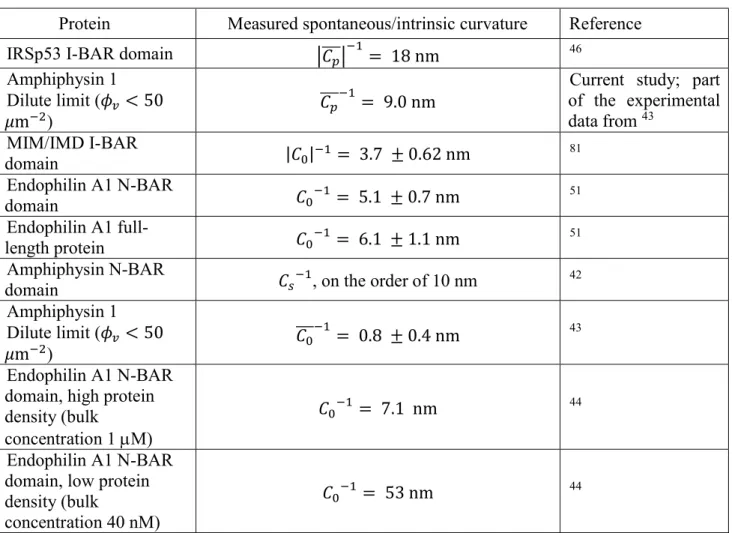
Recent theoretical and experimental works have provided insights in the mechanisms of protein sorting and organization on curved membranes, and how protein binding affects the mechanical properties of the membranes 6, 7, 10, 37, 90. Table 3 summarizes some measurements of
the spontaneous curvature 𝐶 of protein-bound membranes and the intrinsic curvature 𝐶 of membrane-bound proteins, for some BAR-domain proteins. Yet, many issues remained to be addressed. For instance, although recent EM studies provided rich information on how BAR domains organized on cylindrical membranes, most of the studies were performed at high protein density. It would be informative to visualize how BAR proteins are organized on cylindrical membranes at low protein density, in which the proteins diffuse and rotate freely. This would deepen our knowledge on how these proteins organize in cellular membranes where the protein density may be lower than those in test tubes. Also, given that there are usually multiple BAR proteins involved in the generation of curved cellular membranes such as in endocytosis, how different BAR proteins organize on curved membranes remains to be solved. Finally, BAR proteins work synergistically with the actin machinery in many cellular processes such as endocytosis, and the formation of filopodia and lamellipodia 41, 91, 92. To advance our understanding
of these cellular processes, it would be essential to decipher the underlying mechanisms of how the BAR protein-actin machinery operates in these processes 92-94.
Protein Measured spontaneous/intrinsic curvature Reference IRSp53 I-BAR domain 𝐶 = 18 nm 46
Amphiphysin 1 Dilute limit (𝜙 < 50 𝜇m )
𝐶 = 9.0 nm
Current study; part of the experimental data from 43 MIM/IMD I-BAR domain |𝐶 | = 3.7 ± 0.62 nm 81 Endophilin A1 N-BAR domain 𝐶 = 5.1 ± 0.7 nm 51 Endophilin A1 full-length protein 𝐶 = 6.1 ± 1.1 nm 51 Amphiphysin N-BAR
domain 𝐶 , on the order of 10 nm 42 Amphiphysin 1
Dilute limit (𝜙 < 50 𝜇m )
𝐶 = 0.8 ± 0.4 nm 43 Endophilin A1 N-BAR
domain, high protein density (bulk
concentration 1 M)
𝐶 = 7.1 nm 44
Endophilin A1 N-BAR domain, low protein density (bulk
concentration 40 nM)
𝐶 = 53 nm 44
Table 3. Spontaneous curvature of protein-bound membranes and the intrinsic curvature of the membrane-bound proteins. 𝐶 : intrinsic protein curvature; 𝐶 : spontaneous membrane curvature; 𝐶 : effective spontaneous membrane curvature; 𝐶 : effective protein spontaneous curvature.
Appendix
Comparing the fits of the spontaneous curvature and the curvature mismatch model To compare the fits of the two models, we performed two statistical tests.
(1) F test. The null hypothesis is that the curvature mismatch (CM) model does not provide a significantly better fit than the spontaneous curvature (SC) model. Given the 5% level of significant, if the p value associated with the F test is less than 0.05, we can reject the null hypothesis, and conclude that the fit of the CM model is significantly better than that of the SC model.
(2) AIC (Akaike Information Criterion), a likelihood‐based goodness-of-fit measure. AIC = 2𝑘 − 2 ln (𝐿), where k is the number of estimated parameters and 𝐿 is the maximum value
of the likelihood function of the model. A lower AIC value indicates less information lost by a given model, i.e. superior goodness-of-fit. To compare models, one has to compute the relative AIC using exp((AICmin− AICi)/2), in which AICmin is the minimum of AIC among the models and
AICi is the AIC value of the ith model. The relative AIC provides a relative (comparing to AICmin)
probability that the ith model minimizes the information lost. Table 4 presents the results of the two statistical test.
Protein areal
fraction (%) AIC p value of F test
Fig. 2B 𝜙 < 0.25 % SC model: 276.768 CM model: 263.489 Relative AIC: 0.00130809 0.000173691 Fig. 2B 0.25 % < 𝜙 < 0.6 % SC model: 132.492 CM model: 115.132 Relative AIC: 0.000169969 0.0000467467 Fig. 3 𝜙 < 0.5 % SC model: 338.46 CM model: 332.032 Relative AIC: 0.0401913 0.0050931 Fig. 3 0.75 % < 𝜙 < 2 % SC model: 270.671 CM model: 268.006 Relative AIC: 0.263788 0.0378176
Table 4. Relative AIC measurements and p values of the F test. CM: curvature mismatch model; SC: spontaneous curvature model.
Experiments Reagents
All lipids, including total brain lipid extract (TBX, 131101P) and brain L-α-phosphatidylinositol-4,5-bisphosphate (PI(4,5)P2, 840046P), were purchased from Avanti Polar Lipids. Alexa Fluor 488 C5-Maleimide (Alexa 488) were purchased from Invitrogen. All the other reagents were purchased from Sigma-Aldrich.
Cryo-EM experiments Vesicle preparation
The salt buffer outside vesicles was 60 mM NaCl and 20 mM Tris pH 7.5. The salt buffer inside vesicles was 50 mM NaCl, 20 mM sucrose and 20 mM Tris pH 7.5.
Briefly, a lipid mixture of TBX supplemented with 5 mole% PI(4,5)P2 was dried with argon gas and placed under vacuum for at least 3hrs. The dried lipid film was resuspended in a salt buffer (50 mM NaCl, 20 mM sucrose and 20 mM Tris pH 7.5) at a concentration of 1 g.L-1.
Protein purification and labeling
Recombinant mouse IRSp53 I-BAR domain was purified and labeled with AX488 dyes as previously described.95
Cryo-EM sample preparation and observation
After incubating the liposomes at 0.1 mg.mL-1 with the BAR domain at 80 nM for 30
minutes, 4 µL of the sample was plunge frozen on a lacey carbon copper electron microscopy grid in liquid ethane. The Cryo-EM grid was thereafter imaged using a 200kV Lab6 TecnaiG2 microscope equipped with a F-416 TVIPS camera.
𝛽2 centaurin experiments GUV preparation
GUVs were prepared by the electroformation method on platinum (Pt) wires. Briefly, 4 l of a lipid mixture dissolved in chloroform was deposited on Pt-wires, followed by drying under vacuum for 30 – 60 min and then by hydrating in a solution of 70 mM NaCl, 100 mM sucrose, and 10 mM Tris, at pH 7.4. A sine AC current was then applied on the Pt-wires at 500 Hz and 280 mV. The GUVs were grown overnight at 4 °C.
For the tube pulling experiments, GUVs were diluted in a salt buffer composed of 100 mM NaCl and 40 mM glucose (buffered with Tris to pH 7.4).
Protein purification and labeling
The purification and fluorescent labelling of centaurin were performed followed by the procedures described in 79.
Conflicts of interest
There are no conflicts to declare. Acknowledgements
The authors thank Coline Prévost for insightful discussions and her former contribution to the work, P. de Camilli (Yale University, USA) for the amphiphysin plasmid, Emma Evergren (Queen’s University Belfast, UK) and Harvey McMahon (MRC Laboratory of Molecular Biology, UK) for the purified centaurin, Pekka Lappalainen (University of Helsinki, Finland) for the I-BAR domain plasmid, and Joanna Podkalicka (Laboratoire Physico-Chimie Curie, Institut Curie) for assisting with the drawing of the graphic abstract. This work was supported by Human Frontier Science Program Organization (RGP0005/2016 to P.B.), and by Institut Curie and Centre National de la Recherche Scientifique (CNRS). The authors greatly acknowledge the Cell and Tissue Imaging (PICT-IBiSA), Institut Curie, member of the French National Research Infractucture France-BioImaging (ANR10-INBS-04). The P.B. group belongs to CNRS consortium CellTiss, to the Labex CelTisPhyBio (ANR-11-LABX0038, ANR-10-IDEX-0001-02) and to Paris Sciences et Lettres (ANR-10-IDEX-0001-02).
References
1. G. Van Meer, D. R. Voelker and G. W. Feigenson, Nat. Rev. Mol. Cell Biol., 2008, 9, 112-124.
2. B. Alberts, Mol Biol Cell, 6th edn., 2017.
3. A. Picco and M. Kaksonen, Curr. Opin. Cell Biol., 2018, 53, 105-110. 4. H. T. McMahon and J. L. Gallop, Nature, 2005, 438, 590-596.
5. J. Zimmerberg and M. M. Kozlov, Nat. Rev. Mol. Cell Biol., 2006, 7, 9-19.
6. T. Baumgart, B. R. Capraro, C. Zhu and S. L. Das, Annu. Rev. Phys. Chem., 2011, 62, 483-506.
7. B. Antonny, Annu Rev Biochem, 2011, 80, 101-123.
8. L. Lversen, S. Mathiasen, J. B. Larsen and D. Stamou, Nat. Chem. Biol., 2015, 11, 822-825.
9. I. K. Jarsch, F. Daste and J. L. Gallop, J. Cell Biol., 2016, 214, 375-387.
10. M. Simunovic, C. Prevost, A. Callan-Jones and P. Bassereau, Philos. Trans. Royal Soc. A, 2016, 374, 20160034.
11. H. Alimohamadi and P. Rangamani, Biomolecules, 2018, 8, 120.
12. V. A. Frolov, A. V. Shnyrova and J. Zimmerberg, Cold Spring Harb. Perspect. Biol., 2011, 3, a004747.
13. W. F. Zeno, K. J. Day, V. D. Gordon and J. C. Stachowiak, Annu. Rev. Biophys, 2020, 49. 14. S. J. Singer and G. L. Nicolson, Science, 1972, 175, 720-731.
15. G. L. Nicolson, Biochim. Biophys. Acta. Biomembr., 2014, 1838, 1451-1466.
16. J. Bernardino de la Serna, G. J. Schutz, C. Eggeling and M. Cebecauer, Front. Cell Dev. Biol., 2016, 4, 106.
17. P. B. Canham, J. Theor. Biol., 1970, 26, 61-81. 18. W. Helfrich, Z. Naturforsch. C, 1973, 28, 693-703. 19. E. Evans, Biophys. J., 1973, 13, 926-940.
20. E. A. Evans, Biophys. J., 1974, 14, 923-931.
21. F. Brochard and J. Lennon, J. de Phys., 1975, 36, 1035-1047. 22. H. Deuling and W. Helfrich, J. de Phys., 1976, 37, 1335-1345. 23. E. Evans and W. Rawicz, Phys. Rev. Lett., 1990, 64, 2094.
24. M. Bloom, E. Evans and O. G. Mouritsen, Q. Rev. Biophys., 1991, 24, 293-397.
25. R. Lipowsky and E. Sackmann, Structure and dynamics of membranes: I. from cells to vesicles/II. generic and specific interactions, Elsevier, 1995.
26. U. Seifert, Adv. Phys., 1997, 46, 13-137.
27. R. Lipowsky, Adv. Colloid Interface Sci., 2014, 208, 14-24. 28. D. Vollhardt, Adv. Colloid Interface Sci., 2014, 208, 1-292.
29. W. Rawicz, K. C. Olbrich, T. McIntosh, D. Needham and E. Evans, Biophys. J., 2000, 79, 328-339.
30. S. Lorenzen, R.-M. Servuss and W. Helfrich, Biophys. J., 1986, 50, 565-572. 31. M. Mitov, 1978.
32. M. M. Kozlov, Spontaneous and Intrinsic Curvature of Lipid Membranes: Back to the Origins, Springer, 2018.
33. P. Bassereau and P. Sens, Physics of Biological Membranes, Springer, 2018.
34. L. Iversen, S. Mathiasen, J. B. Larsen and D. Stamou, Nat. Chem. Biol., 2015, 11, 822. 35. P. Bassereau, R. Jin, T. Baumgart, M. Deserno, R. Dimova, V. A. Frolov, P. V. Bashkirov,
Pucadyil, W. F. Zeno, J. C. Stachowiak, D. Stamou, A. Breuer, L. Lauritsen, C. Simon, C. Sykes, G. A. Voth and T. R. Weikl, J. Phys. D Appl. Phys., 2018, 51, 343001.
36. P. J. Carman and R. Dominguez, Biophys. Rev., 2018, 10, 1587-1604.
37. M. Simunovic, E. Evergren, A. Callan-Jones and P. Bassereau, Annu Rev Cell Dev Biol., 2019, 35, 111-129.
38. J. Saarikangas, H. Zhao, A. Pykäläinen, P. Laurinmäki, P. K. Mattila, P. K. Kinnunen, S. J. Butcher and P. Lappalainen, Curr. Biol., 2009, 19, 95-107.
39. B. Qualmann, D. Koch and M. M. Kessels, EMBO J., 2011, 30, 3501-3515. 40. S. Suetsugu, J. Electron Microsc., 2016, 65, 201-210.
41. T. Nishimura, N. Morone and S. Suetsugu, Biochem. Soc. Trans., 2018, 46, 379-389. 42. M. C. Heinrich, B. R. Capraro, A. Tian, J. M. Isas, R. Langen and T. Baumgart, J. Phys.
Chem. Lett., 2010, 1, 3401-3406.
43. B. Sorre, A. Callan-Jones, J. Manzi, B. Goud, J. Prost, P. Bassereau and A. Roux, PNAS, 2012, 109, 173-178.
44. C. Zhu, S. L. Das and T. Baumgart, Biophys J, 2012, 102, 1837-1845.
45. W.-T. Hsieh, C.-J. Hsu, B. R. Capraro, T. Wu, C.-M. Chen, S. Yang and T. Baumgart, Langmuir, 2012, 28, 12838-12843.
46. C. Prevost, H. Zhao, J. Manzi, E. Lemichez, P. Lappalainen, A. Callan-Jones and P. Bassereau, Nat. Commun., 2015, 6, 8529.
47. M. Galic, S. Jeong, F.-C. Tsai, L.-M. Joubert, Y. I. Wu, K. M. Hahn, Y. Cui and T. Meyer, Nat. Cell Biol., 2012, 14, 874-881.
48. M. Kaksonen and A. Roux, Nat. Rev. Mol. Cell Biol., 2018, 19, 313-326.
49. J. J. Thottacherry, M. Sathe, C. Prabhakara and S. Mayor, Annu. Rev. Cell Dev. Biol., 2019, 35.
50. A. Breuer, L. Lauritsen, E. Bertseva, I. Vonkova and D. Stamou, Soft Matter, 2019, 15, 9829-9839.
51. Z. Shi and T. Baumgart, Nat. Commun., 2015, 6, 5974. 52. V. Markin, Biophys. J., 1981, 36, 1-19.
53. S. Leibler, J. Phys., 1986, 47, 507-516.
54. R. Lipowsky, Faraday Discuss., 2013, 161, 305-331.
55. F. Campelo and M. M. Kozlov, PLoS Comput. Biol., 2014, 10, e1003556. 56. S. Svetina, Eur. Biophys. J., 2015, 44, 513-519.
57. T. S. Krishnan, S. L. Das and P. S. Kumar, Pramana – J. Phys., 2020, 94, 1-7. 58. M. Kozlov and W. Helfrich, 1992, 8, 2792-2797.
59. M. Mally, B. Božič, S. V. Hartman, U. KlanÄ nik, M. Mur, S. Svetina and J. Derganc, 2017, 7, 36506-36515.
60. F. Campelo, H. T. McMahon and M. M. Kozlov, Biophys. J., 2008, 95, 2325-2339. 61. V. Kralj-Iglic, S. Svetina and B. Zeks, Eur. Biophys. J, 1996, 24, 311-321.
62. K. R. Rosholm, N. Leijnse, A. Mantsiou, V. Tkach, S. r. L. Pedersen, V. F. Wirth, L. B. Oddershede, K. J. Jensen, K. L. Martinez, N. S. Hatzakis, P. M. Bendix, A. Callan-Jones and D. Stamou, Nat. Chem. Biol., 2017, 13, 724.
63. B. Božič, S. L. Das and S. Svetina, Soft Matter, 2015, 11, 2479-2487.
64. A. Frost, R. Perera, A. Roux, K. Spasov, O. Destaing, E. H. Egelman, P. De Camilli and V. M. Unger, Cell, 2008, 132, 807-817.
65. C. Mim, H. Cui, J. A. Gawronski-Salerno, A. Frost, E. Lyman, G. A. Voth and V. M. Unger, Cell, 2012, 149, 137-145.
66. J. Adam, N. Basnet and N. Mizuno, Sci. Rep., 2015, 5, 1-15. 67. P. Girard, J. Prost and P. Bassereau, 2005, 94, 088102.
68. S. Aimon, A. Callan-Jones, A. Berthaud, M. Pinot, G. E. Toombes and P. Bassereau, Dev. Cell, 2014, 28, 212-218.
69. R. Shlomovitz and N. Gov, Phys. Biol., 2009, 6, 046017.
70. R. Shlomovitz, N. Gov and A. Roux, New J. Phys., 2011, 13, 065008.
71. S. Suetsugu, S. Kurisu and T. Takenawa, Physiol. Rev., 2014, 94, 1219-1248. 72. Y. Senju and P. Lappalainen, Curr. Opin. Cell Biol., 2019, 56, 7-13.
73. A. Disanza, S. Bisi, M. Winterhoff, F. Milanesi, D. S. Ushakov, D. Kast, P. Marighetti, G. Romet-Lemonne, H.-M. Müller, W. Nickel, J. Linkner, D. Waterschoot, C. Ampè, S. Cortellino, A. Palamidessi, R. Dominguez, M.-F. Carlier, J. Faix and G. Scita, EMBO J., 2013, 32, 2735-2750.
74. M. Gleisner, B. Kroppen, C. Fricke, N. Teske, T.-T. Kliesch, A. Janshoff, M. Meinecke and C. Steinem, J. Biol. Chem., 2016, 291, 19953-19961.
75. A. Zemel, A. Ben-Shaul and S. May, J. Phys. Chem. B, 2008, 112, 6988-6996.
76. A. Roux, G. Koster, M. Lenz, B. Sorre, J.-B. Manneville, P. Nassoy and P. Bassereau, PNAS, 2010, 107, 4141-4146.
77. E. Ambroggio, B. Sorre, P. Bassereau, B. Goud, J. B. Manneville and B. Antonny, EMBO J, 2010, 29, 292-303.
78. B. R. Capraro, M. C. Heinrich, Y. Yoon, W. Cho and T. Baumgart, Biophys. J., 2010, 98, 284a.
79. M. Simunovic, E. Evergren, I. Golushko, C. Prévost, H.-F. Renard, L. Johannes, H. T. McMahon, V. Lorman, G. A. Voth and P. Bassereau, PNAS, 2016, 113, 11226-11231. 80. M. Simunovic, J.-B. Manneville, H.-F. Renard, E. Evergren, K. Raghunathan, D. Bhatia,
A. K. Kenworthy, G. A. Voth, J. Prost, H. T. McMahon, L. Johannes, P. Bassereau and A. Callan-Jones, Cell, 2017, 170, 172-184.
81. Z. Chen, Z. Shi and T. Baumgart, Biophys. J., 2015, 109, 298-307.
82. C. Prevost, F.-C. Tsai, P. Bassereau and M. Simunovic, JoVE, 2017, e56086.
83. B. J. Peter, H. M. Kent, I. G. Mills, Y. Vallis, P. J. G. Butler, P. R. Evans and H. T. McMahon, Science, 2004, 303, 495-499.
84. B. Daum, A. Auerswald, T. Gruber, G. Hause, J. Balbach, W. Kühlbrandt and A. Meister, J. Struct. Biol., 2016, 194, 375-382.
85. W. F. Zeno, W. T. Snead, A. S. Thatte and J. C. Stachowiak, Soft Matter, 2019, 15, 8706-8717.
86. X. Pang, J. Fan, Y. Zhang, K. Zhang, B. Gao, J. Ma, J. Li, Y. Deng, Q. Zhou and E. H. Egelman, Dev. Cell, 2014, 31, 73-86.
87. Z. Jarin, F.-C. Tsai, A. Davtyan, A. J. Pak, P. Bassereau and G. A. Voth, Biophys. J., 2019, 117, 553-562.
88. B. Nepal, A. Sepehri and T. Lazaridis, BioRxiv, 2020.
89. Z. Jarin, A. J. Pak, P. Bassereau and G. A. Voth, 2021, 120, 46-54.
90. N. Ramakrishnan, R. P. Bradley, R. W. Tourdot and R. Radhakrishnan, J. Phys. Condens. Matter, 2018, 30, 273001.
91. S. Suetsugu and A. Gautreau, Trends Cell Biol., 2012, 22, 141-150. 92. N. Gov, Philos. Trans. R. Soc. Lond., B, Biol. Sci., 2018, 373, 20170115.
93. L. Mesarec, W. Góźdź, V. K. Iglič, S. Kralj and A. Iglič, Colloids Surf. B, 2016, 141, 132-140.
94. S. Brühmann, D. S. Ushakov, M. Winterhoff, R. B. Dickinson, U. Curth and J. Faix, PNAS, 2017, 114, E5815-E5824.
95. J. Saarikangas, H. Zhao, A. Pykalainen, P. Laurinmaki, P. K. Mattila, P. K. Kinnunen, S. J. Butcher and P. Lappalainen, 2009, 19, 95-107.