Relationships between anatomical and vibrational properties of wavy sycamore maple

HAL Id: hal-01667816

https://hal.umontpellier.fr/hal-01667816

Submitted on 19 Dec 2017

HAL is a multi-disciplinary open access archive for the deposit and dissemination of sci-entific research documents, whether they are pub-lished or not. The documents may come from teaching and research institutions in France or abroad, or from public or private research centers.

L’archive ouverte pluridisciplinaire HAL, est destinée au dépôt et à la diffusion de documents scientifiques de niveau recherche, publiés ou non, émanant des établissements d’enseignement et de recherche français ou étrangers, des laboratoires publics ou privés.

properties of wavy sycamore maple

Ahmad Alkadri, Capucine Carlier, Imam Wahyudi, Joseph Gril, Patrick

Langbour, Iris Brémaud

To cite this version:

Ahmad Alkadri, Capucine Carlier, Imam Wahyudi, Joseph Gril, Patrick Langbour, et al.. Relation-ships between anatomical and vibrational properties of wavy sycamore maple. IAWA Journal, Brill publishers, 2018, 39 (1), pp.63-86. �10.1163/22941932-20170185�. �hal-01667816�

Relationships between Anatomical and Vibrational

Properties of Wavy Sycamore Maple

Authors:

Ahmad Alkadri

, Capucine Carlier

, Imam Wahyudi

, Joseph Gril

,

Patrick Langbour

, Iris Brémaud

Affiliations:

1_{Wood Team, Laboratory of Mechanics and Civil Engineering – LMGC, CNRS, UMR 5508,}

Université de Montpellier - CC048,163 rue Auguste Broussonnet, 34090 Montpellier, France

2_{Department of Forest Products, Faculty of Forestry, Bogor Agricultural University,}

Dramaga, 16680 Bogor, Indonesia

3_{BioWooEB Research Unit, CIRAD, TA B-114/16, 73 Rue Jean-François Breton, 34398}

Montpellier Cedex 5, France

* Corresponding author, ahmad.alkadri@outlook.com

Final Version:

http://booksandjournals.brillonline.com/content/journals/10.1163/22941932-20170185 Citing for scientific matters should always refer to the final version of this article.

Abstract

Sycamore maple (Acer pseudoplatanus L.) is a wood species particularly known for its wavy grain figure and its high-value utilization among luthiers and craftsmen for making musical instruments or furniture. In this study, the anatomical and physical-acoustical characteristics of its wood, taken from different trees with various surface figure, were characterized. Vibrational mechanical measurements were conducted taking into account radial and longitudinal directions and local variations, waviness’ parameters were quantified on split blocks, and anatomical properties such as microfibril angle and rays’ dimensions were measured using light microscopy. Results provide a complete dataset on the properties of sycamore maple showing a gradient of wavy figure. Through statistical analysis, it can be concluded that there exist significant correlations between the measured parameters, particularly between waviness and microfibril angle, and between these anatomical features and the specific modulus of elasticity and damping by internal friction of the wood in longitudinal direction. Anisotropy was found to be very low but was not satisfactorily explained by the studied anatomical features. Prospects for future studies on wavy figure are introduced.

Keywords: anisotropy, damping, microfibril angle, specific modulus of elasticity, rays, wavy

grain

Symbols and Abbreviations

For this article, the following symbols and abbreviations apply.

A amplitude (mm)

ρ density (g/cm3)

γ specific gravity, without unit

E’ Young’s modulus of elasticity (GPa)

E’/γ specific modulus of elasticity expressed using specific gravity (GPa)

E’/ ρ specific modulus of elasticity expressed using density (MPa m3 kg-1)

E’L/ ρ E’/ρ parallel to the grain or longitudinal

E’R/ ρ E’/ρ perpendicular to the grain or radial

fR resonance frequency (Hz)

λ wavelength, (mm) LRH large rays’ height (µm)

LRW large rays’ width (µm) MFA microfibril angle (°)

PLRTA ratio between large rays’ surface area and total area in tangential section (%) PSRTA ratio between large rays’ surface area and total area in tangential section (%) RH relative humidity (%)

SRH small rays’ height (µm) SRW small rays’ width (µm) tanδ damping coefficient

tanδL damping coefficient parallel to the grain or longitudinal

tanδR damping coefficient perpendicular to the grain or radial

θ grain angle (°)

θaverage average value of grain angle or average slope (°)

θmax maximum value of grain angle or maximum slope (°)

v sound speed (m/s)

w waviness

Introduction

Wood can present a variety of figure, which are both highly sought after for high-end uses and still little understood from the point of view of their biological origins and/or of their physical-mechanical consequences. Wood figures can be defined by the proportion of different anatomical elements (i.e. texture) and/or by the orientation of “grain” (i.e. orientation of fibres with respect to the trunk axis) such as in interlocked or wavy grain (Beals and Davis 1977; Harris 1989). Wavy or curly figure is highly valued, and maple wood presenting this figure is particularly famous. Wavy maple, especially sycamore maple (Acer pseudoplatanus L.), is also referred to as “fiddleback” based on its favored utilization as the back plates and other parts of string musical instruments such as violin and guitar by the instrument makers and artisans. The presence of these wavy grains raises the value of the wood aesthetically and thus it is also used in a decorative use for furnitures (Beals & Davis 1977). Well figured maple wood reaches very high prices. Based on reports from Slovenia, for example, the wavy maple’s prices are consistently highest among the wood auctioned (Kobal et al. 2013; Krajnc et al. 2015). However, only a small percentage of trees exhibit a pronounced wavy figure.

Due to the rarity and high value brought by the presence of this wavy grain, several studies in the past have tried to determine the factors affecting its formation. For example: genetical

factors, implying that it can be successfully reproduced through vegetative propagation (Rohr & Hanus 1987); external stresses (Ewald & Naujoks 2015); and phytohormones like auxin and ethylene (Nelson & Hillis 1978). Efforts in reproducing these traits in sycamore maple and other wood species through vegetative propagation have been conducted and are ongoing (Bailey 1948; Ryynänen & Ryynänen 1986; Rohr & Hanus 1987; McKenna et al. 2015; Ewald & Naujoks 2015). Regarding the mechanism of formation, the most widely accepted theory states that cambium cells’ orientation is the primary factor in the formation of wavy grain (Hejnowicz & Romberger 1973; Savidge & Farrar 1984; Harris 1989). However, it is not fully clear yet how this re-orientation of cambium cells is affected by genetics, as waviness appears to be heritable, and as environment is one of the factors causing its expression (Harris 1989). This hypothesis has been explored in several publications (Savidge & Farrar 1984; Harris 1989; Kramer 2006).

As has been stated before, wavy sycamore is most famously used by musical instrument makers for back plates of string instruments such as violins and guitars (Bucur 2006). Acoustically speaking, properties that are important for instrument plates are density (ρ), Young’s modulus (E’), specific modulus (E’/ρ, which is related to the sound speed V≈[ E’/ρ]1/2), damping coefficient (tanδ), and their anisotropy between longitudinal (L) and radial (R) directions (Ono & Norimoto 1983; Obataya et al. 2000; Bucur 2006). The woods used for back plates—like maple—are known to show different values of these properties than wood for top-plates such as spruce (Yano et al. 1992; Wegst 2006; Yoshikawa 2007). Other studies have suggested that the craftsmen tend to select their wood based also on visual and cultural preferences (Buksnowitz et al. 2007; Carlier et al. 2014), thus strengthening the wavy sycamore’s aesthetical value. Few publications have actually compared mechanical and acoustical properties of maple wood with or without wavy grain, and results are somewhat inconsistent: some of them suggest that wavy wood would have higher density, and higher or similar Young’s modulus, than non-wavy wood, some of them suggest different trends (Bucur 2006; Spycher et al. 2008; Kudela & Kunstar 2011). However, most studies are based on the comparison of one or two samples of each type of wood only, and full sets of characteristics (including anisotropic mechanical properties and anatomical features) are still missing. This can be partly attributed to the rarity of wood with wavy grain in nature and its high costs, making it difficult to be obtained for more exhaustive research.

As has been stated also by Bucur (2006), it is necessary to conduct more experiments to relate the physical, mechanical and acoustical properties of sycamore maple wood to characteristics of waviness at the macro- and microscopic level; hence the need for anatomical

investigations. In the past, others have studied the relationships between the anatomical properties of the wood with its physical and mechanical properties. The microfibril angle MFA (in straight-grained wood) and the fiber angle (or grain angle) strongly affect the vibrational mechanical properties such as E’/ρ and tand in L direction (Obataya et al. 2000; Brémaud et al. 2011), while the rays may affect the mechanical and physical properties in R direction (Burgert & Eckstein 2001; Reiterer et al. 2002). However, these three different groups of anatomical features are seldom considered together in relation to the physical-mechanical-acoustical properties of the wood.

Therefore, this research aims to better characterise sycamore maple wood presenting a gradient of wavy figure, and to determine the potential correlations between anatomical features (wavy grain, microfibril angle, rays’ characteristics) and physical, mechanical, and acoustical properties (including specific modulus of elasticity and damping coefficient and their anisotropy). The sample selection will include a wide diversity of wood surfaces which, in theory, possess a varying level of grain waviness, thus making it possible to determine the relationships between those parameters with statistical analysis.

Materials and Methods

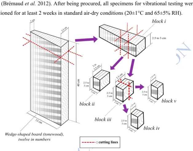
Specimen Preparation

Twelve quarter-cut wedge shaped boards for violin back plates, labelled A to L, were used in this study, with the approximate dimensions of ± 40 cm × 13 cm × 2.5 cm (connecting side) or 1 cm (edge). They were obtained from several violin makers and specialized wood suppliers from Romania, Bosnia and France. Specimens from each board were prepared according to Figure 1. The first cut produced a trapesium-shaped block 2.5—3 cm high in longitudinal (L) direction, named block i. From block i, second cuttings were conducted to produce block ii and

block iii, with dimensions 2 cm × 2.5 cm × 3 cm. Each block ii from each specimen were used

for waviness measurement. Block iii were then cut again to produce block iv and block v used for MFA and ray dimensions measurement, respectively.

For vibrational properties measurement, using the existing sampling plan that was also used in other assessments of within-plate variability (Carlier et al. 2014) using vibrational tests (Bré-maud et al. 2010, 2012), the boards were cut into small strip specimens with the dimension of (150×12×2 mm3) (L×R×T) for longitudinal specimens, and (120×12×2 mm3) (R×L×T) for ra-dial specimens (Figure 2). This sampling plan allows us to study the distribution of properties

within plates.The variation of specimen thickness must be reduced as much as possible for it provides a primary source of errors in the measurement of the specific modulus of elasticity (E’/ρ) (Brémaud et al. 2012). After being procured, all specimens for vibrational testing were conditioned for at least 2 weeks in standard air-dry conditions (20±1°C and 65±5% RH).

Figure 1: Specimen preparation from the wedge-shaped board toward the small blocks needed for MFA and ray dimensions measurement

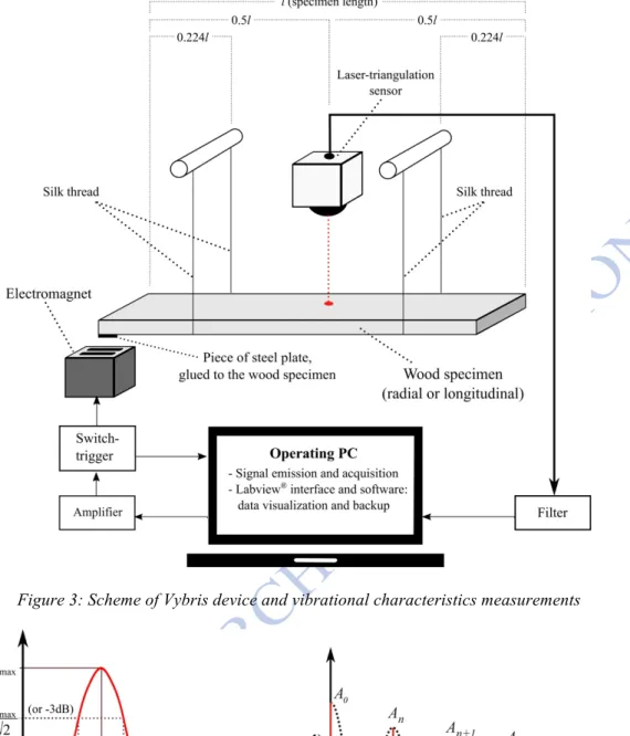
Vibrational Measurement

The measurement of vibrational properties of the specimens was conducted based on the prin-ciple of non-contact forced vibrations of free-free slender beams (Obataya et al. 2000; Ono & Norimoto 1983) using a semi-automated device “Vybris” which was developed and manufac-tured in LMGC (Laboratoire de Mécanique et Génie Civil) in Montpellier, France (Brémaud 2006). For the measurement, the wood specimen was hung with silk threads, vibrated using an electromagnet facing a thin steel piece glued to one end of the sample, and the vibration was then recorded by a laser-triangulation sensor with the resolution (smallest measurable displace-ment or vibration amplitude) of 10 µm (Figure 3). The testing was conducted through a program specifically developed with Labview® (Brémaud et al. 2012). Two parameters were deter-mined: E’/ρ and tanδ. A frequency sweep detects the resonance frequency (fR), and E’/ρ is

determined using the Euler-Bernoulli equation (equation 1) (Brémaud et al. 2012):

E’/ρ = [(48 . p2 _{. l}4_{) / (m}

n4 . h2)] × fRn2 (equation 1)

where l is the specimen’s length, h is the specimen’s thickness, fRn is the resonance frequency

of the mode n and mn is a constant based on the order of the mode (here we used m1=4.730).

The tanδ is then determined in the frequency domain and the time-domain.

In the frequency domain, tanδ is determined using a frequency scan through the bandwidth (Df) at half-power of the resonance curve (-3dB) (Figure 4a). The value obtained through this method also often called as the quality factor (Q-1), determined as the ratio between Df (f2-f1)

and fR (equation 2).

Q-1 = (f2−f1)/fR = Df/fR ≈ tand (equation 2)

While in the time domain, tanδ is determined through the logarithmic decrement (L) of amplitudes after the stopping of the excitation, fixed at fR. The L is determined using the

vibration amplitudes of two successive peaks (Figure 4b) (equation 3): L = (1/n) × ln(A0/An) ≈ p × tand

tand ≈ L/p (equation 3)

The value of tand determined through frequency and time domain should be equivalent (tand≈Q−1_{≈ L/π) for values <<0.1 (Jones 2001, Brémaud et al. 2012).}

Figure 3: Scheme of Vybris device and vibrational characteristics measurements

Figure 4: Determination of tand the frequency (a) and time (b) domains

Two scans were performed in the measurement of each single specimen. In the first one, a wide frequency range (150—750 Hz for longitudinal (L) specimens and 80—500 Hz for radial (R) ones) was emitted and the resulting vibration is measured to identify the first resonant fre-quency (fR). Afterward, a second scan was conducted using a narrower range of frequency

done for each specimen, with experimental error being ≤2.5% and presented values are the average ones.

MFA Measurement

Specimens for MFA measurement were prepared based on the light microscopy MFA methods described by Senft and Bendtsen (1985). The blocks used for MFA measurements were those of block iv. Each of them were submerged in water, taken out, oven-dried, and then re-sub-merged again. This cycle was conducted at least two times in order to create cracks within the wood cells which will enhance the appearance of MFA.

Sectioning was conducted on the blocks’ radial surface using a rotary-slide microtome to produce small thin sections approximately 15 µm thick. The resulting sections were stored in 50% alcohol. Afterwards, the sections were dehydrated in a solution of absolute (>99%) alcohol for 5 min and then taken out and left drying for approximately 30 s. This dehydration step was conducted twice. The sections were then immersed in a solution of 2% iodine-potassium iodide (IKI) for 2 to 10 s. Then, sections were placed on a slide and excess solution were blotted using a paper towel. Two drops of 60% nitric acid (HNO3) were added to the section before applying

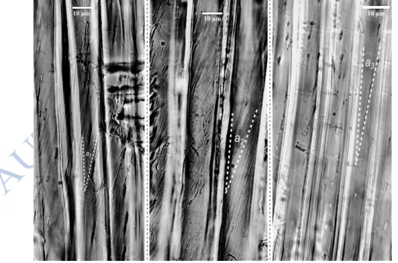
a coverslip. The iodine will fill the cracks between the microfibrils, thus making the MFA vis-ible as dark streaks along the cell wall. Pictures of the MFA were taken using a digital camera Nikon DS Fi1 associated with a light microscope (Olympus BX6) with 600× enlargement. The angles were measured using ImageJ, and for each specimen, the number of measurements ranges from 40 to 146 times depending on the clarity of MFA appearance. On specimens with low clarity of MFA appearance, the measurements were conducted in higher number of times compared to the specimens with high clarity of MFA appearance. This was done to lower the possibility of errors.

During the course of the measurements, because of the different surface cut condition of each sample, the angles measurements were not always conducted according to the same strict rule. The MFA themselves are very hard to be observed directly using light microscopy because the fibrils in the cell walls, especially in S2 layer, are tightly formed (Long et al. 2000). The pretreatment given before the slicing relieved the tightness a little, but not by a wide margin, and thus the resulting surfaces made it necessary to measure the MFA using one of the following techniques:

a. the MFA was measured according to the angle of the cracks between microfibrils and complemented by the angle of the pits (Donaldson 2007),

b. the MFA was measured according to the MFA directly. This rarely occurred, for in order to be able to observe and measure the MFA using light microscopy, the “cracking” or defibrillation between the microfibrils must happened exactly between each one of them within one fiber cells. These rare occurrences could be chalked up to the low tightness between the microfibrils and the low amount of lignin or bonds between the MFA,

c. the MFA was measured based on the angle of the pits within the fiber (Donaldson 2007). This is an acceptable method of MFA measurement, but it has to be conducted very carefully because the angle of the pits does not always correspond perfectly with the MFA. Thus, it is necessary to measure more than one pits’ angle within the same fiber, and to check with the occurring cracks, however small they are, within the same or neighboring cells. If the angles between them are consistent and not vary by a high amount, then the angle of the pits can be said to be similar, or the same, with the MFA. Also observed were the “tails” of the pits, or the elongated lines from both end of the pits, which normally correspond more with the MFA than the “body” of the pits. Another particular condition here is that most of the specimens possess wavy grain. This made the MFA measurement more difficult because the changing grain angle also often distorts the appearance of MFA on a section. Therefore, location choices are also important to note. Most of the measured MFA are the ones who appear clear or not distorted. It means that the grain angle where the MFA were measured must be low or closer to zero, indicating that they’re on the top of the peak or hill (the amplitude point, where the grain angle is close to 0º) of the wavy grain.

Ray Dimensions Measurement

The blocks used for ray dimensions measurements were those of block v. Each blocks’ tangential surfaces were sectioned using a rotary-slide microtome to small sections 15—17.5 µm thick. The resulting sections were stored in 50% alcohol. Afterwards, sections were immersed in sodium hypochlorite for 30 minutes to solubilize the extractives. The sections were then immersed in colorant (green iodine, prepared with 1g Iodine powder + 30 cm3 distilled water and 70 cm3 ethanol), giving it a green color to enhance the observation. Next, sections were dehydrated in several levels of alcohol solution, starting from 25%, 50%, 75%, towards absolute (>99%). Fully dehydrated, sections were placed on a slide and given a coverslip. Pictures were taken using a light microscope with 40× enlargement and the rays’ dimensions

were measured using ImageJ.

Measured parameters were the height and width of, respectively, large rays and small rays, and the percentage of the surface of the section they represent. The categorization of large rays and small rays are based on their diameter. On average, the diameter of a single ray cell of the sycamore maple is approximately 15.5 µm (Schoch et al. 2004), thus if the rays’ width exceeds 31 µm, or if it has more than 2 seriates, it will be categorized as large rays while the ones which possess less than or equal to 2 seriates will be categorized as small rays. The number of measurements of large rays’ dimensions range from 53 to 138 times per specimens, while the small rays’ range from 219 to 578. Similar with MFA measurements, the clearer the rays’ appearance of a specimen, the lower the number of measurements conducted.

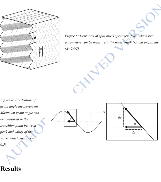
Wavy Figure and Grain Angle Measurement

Block ii were split parallel to the grain direction (Figure 5). The resulting splits show clear

wave-like figures which was then scanned and the wavelength and amplitude were measured using ImageJ. In order to measure the wavy grain, it is assumed that: a) the wave-like figures are consistent throughout the part of the wood which possesses it, b) the wave-like figures fol-low the standard equation form of a sinusoidal wave (equation 4) with two parameters taken into account: the amplitude (A) and wavelength (l).

! = # sin'()_* (equation 4)

In a sinusoidal wave function, the slope of a specific point (x,y) can be calculated as dy/dx (Figure 6). Slope = tanθ with θ in radians (rad) unit. Thus, for θ in degrees (°) unit:

+ = (180/1)×tan−1_{(7!/78) (equation 5)}

When the slope is small, or if dy

dx << 1 , such is the condition here, the slope ≈ θ (rad), and:

è qaverage (rad) ≈ average slope

è qaverage (º) ≈ 180/p × average slope (equation 6)

(equation 7) θ max can be observed in x = 0.5l Therefore:

(equation 8) Thus, we can express the degree of waviness, or ‘how wavy’ the wood is, through the calculation of average grain angle (θaverage, equation 7) and max grain angle (θmax, equation 8).

The grain angle (θ) is calculated because it has been known to strongly influence the mechanical and physical characteristics in wood, and thus the results will be valuable for further experi-ments and as a reference for other studies in this field.

Moreover, a third way to express the degree of waviness is by simply calculating the ratio between the A and λ, as shown in equation 9. This value is also written as waviness (w) and, as can be clearly seen, derived from the θaverage (equation 7). It is simpler to calculate and the value

can be used to visualize the wood’s waviness better.

9 = #/; (equation 9)

Statistical Analysis

Statistical analysis was conducted using Microsoft Excel 2011 and R with Rstudio 0.99.902 as its operating interface. For anatomical measurements (MFA, waviness, rays) which are based on a high number of observations per sample plate, basic statistics on their distribution were conducted (average, median, percentile repartition, confidence interval and outliers). Then, for the analysis of relations between all measured parameters, linear correlations were analyzed using Pearson product-moment coefficient of correlation (r) and coefficient of determination

(R2 or r2), which indicates the proportion of the variance in the dependent variable that is predictable from the independent variable. After the r has been determined, its significance was tested using p-value, which was then compared to the specified value for the considered degree of freedom (= number of samples – 2). In this study, we use the degree of confidence of 5%, which means that if the p-value is lower than 0.05, the r between the two datasets will be regarded as indicating a significant correlation.

Figure 5: Depiction of split block specimen, from which two parameters can be measured: the wavelength (λ) and amplitude (A=2A/2)

Figure 6: Illustration of grain angle measurement. Maximum grain angle can be measured in the transition point between peak and valley of the wave, which means x = 0.5λ

Results

Vibrational Properties

Results from the vibrational measurements on all specimens show that, overall, the relationship between tanδ and E’/ρ of sycamore maple (Figure 7) follows a trend similar to the “standard”

However, in L direction, tanδL of the waviest specimens tends to be higher than the standard.

While in R directions, both E’R/ρ and tanδR of all tested maple tend to be smaller (Figure 7).

Figure 7: Vibrational property results for both R and L directions and the comparison between the relationship found between internal friction tanδ and E’/ρ as obtained on all 139 specimens of sycamore maple measured in this study with the “standard” relationship established on numerous species (Ono & Norimoto 1983; Brémaud

et al. 2012).

Figure 8: Local variations (of specimens from each plate) of E’/ρ and tanδ of L specimens. Location no. 1 is closer to the pith and no. 7 is closer to the bark in the tree. Continuous red line indicates the average trend over

all plates.

Further analysis on local variations also shows that, along the trunk’s radius, E’L/ρ tends to

increase and tanδL to decrease the further the wood is from the pith (Figure 8). On the other

to the observations, the part of the wood closer to the bark tends to have higher E’L/ρ and lower

tanδL. It must be noticed that, due to the origin of the plates (wedge-shaped boards prepared for

violin making), the exact distance to the pith or bark is unknown. However, those trends do not show high significance.

When considering the average values of vibrational properties per plate (Table 1), longitudinal properties vary from 9.7 to 19.7 GPa for E’L/ρ and from 0.0085 to 0.0156 for tanδL.

By comparison, the average values over 105 species of temperate hardwoods are of 17 GPa for

E’L/ρ and of 0.0103 for tanδL (Brémaud 2012). Radial properties vary from 1.9 to 3.0 GPa for

E’R/ρ and from 0.022 to 0.026 for tanδR. As a results, ratios of anisotropy range from 4.0 to 7.3

for specific modulus E'/ρ (L/R) and from 1.7 to 2.8 for damping tanδ (R/L). Wavy sycamore maple is less anisotropic than other hardwood species, for which the average anisotropic ratios are 7.8 (L/R) for specific modulus E'/ρ and of 2.7 (R/L) for damping tanδ (Brémaud et al. 2011).

Microfibril Angle

The measurement results, as presented in table 2, show that the 12 plates used in this study possess a wide variability of MFA with different appearances. This conforms with the planned MFA measurement methods that have been proposed before by Donaldson (2007). Results show that the average MFA per plate ranges from 8.7° to 20.4° (Table 2).

Figure 9: MFA measurement methods, from left to right, a) using the angle of the cracks and pit apertures, b) the MFA directly, visible after stained with iodine, c) angle of the pit apertures, which are small but still

Waviness

The amplitude A and wavelength λ for each sample plate are presented in Table 3. The A for each plate ranges from 0.14 mm to 0.31 mm, λ from 6.11 mm to 18.07 mm. From those A and

λ the value of waviness w and grain θ was calculated and the results are also shown in table 3.

The waviness of the grain (w) differs markedly among plates, ranges from 0.008 to 0.049. Fur-thermore, the θ also ranges from 2.75º to 19.54º, with more than 700% difference between the lowest and the highest θ.

Ray Dimensions

The ray characteristics measured in this study consist of ray height, width, and proportion of area occupied by rays. The measurement was conducted on the tangential section. It is observed that the sycamore maple possesses uniseriate and multiseriate rays: in addition to uniseriate rays, large rays consisting of up to 6—8 ray cells are also present and visible to the naked eyes. This confirms the previous study on the anatomical aspect of wavy sycamore maple in France (Keller 1992).

The measurement results are presented in table 3. Although visually it seems that the rays in wood with wavier grain possess lower height and more tightly packed (the frequency per-centage is larger), based on the statistical analysis (Table 4), there is no significant correlation between the degree of grain waviness with rays’ dimensions.

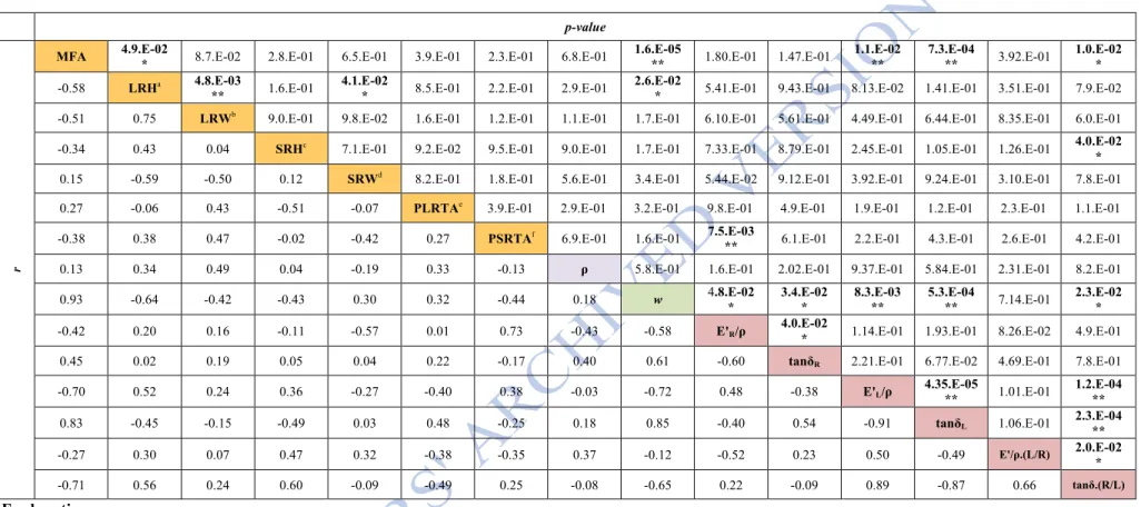
Correlation Between Parameters

The correlation matrix (Table 4) indicates significant correlations between some vibrational-mechanical and anatomical characteristics of the maple wood with different degrees of wavi-ness. Those significant correlations are: MFA and w, Large Rays' height and w, tanδ of L spec-imens (tanδL) with MFA, tanδL with w, tanδ of R specimens (tanδR) with w, specific modulus

of L specimens (E’L/ρ) with MFA, E’L/ρ with w, and Young's modulus of L specimens (E’L)

with w. The highest correlation is observed between MFA and w: the larger the waviness, the higher the MFA. Following the correlation test, linear multiple regression analysis was also conducted for tanδL with MFA and w, and for E’L/ρ with MFA and w (Table 5 and 6).

Table 1. Measurement results of the sycamore maple wood’s physical and vibrational properties Parameters Plates A B C D E F G H I J K L ρ (g/cm3₎ [n] [13] [15] [12] [12] [13] [14] [14] [14] [13] [12] [12] [11] m 0.655 0.688 0.588 0.664 0.637 0.618 0.631 0.588 0.643 0.693 0.552 0.626 (σ) (0.025) (0.012) (0.008) (0.015) (0.009) (0.012) (0.015) (0.014) (0.012) (0.012) (0.007) (0.013) E'R/ρ (GPa) [n] [5] [5] [4] [4] [5] [5] [5] [5] [4] [4] [4] [4] m 2.98 2.69 2.83 2.75 1.92 2.82 2.82 2.89 2.87 2.09 3.02 2.36 (σ) (0.11) (0.19) (0.03) (0.08) (0.10) (0.08) (0.08) (0.15) (0.06) (0.06) (0.05) (0.07) tanδR (×1000) [n] [5] [5] [4] [4] [5] [5] [5] [5] [4] [4] [4] [4] m 22.1 22.4 24.0 23.1 24.1 23.0 23.0 20.8 20.9 25.5 21.7 21.5 (σ) (0.4) (0.6) (0.6) (0.4) (0.8) (0.5) (0.5) (0.3) (0.7) (2.7) (1.5) (1.0) E'L/ρ (GPa) [n] [8] [10] [8] [8] [8] [9] [9] [9] [9] [8] [8] [7] m 17.4 15.5 11.4 15.2 13.8 17.2 20.7 15.9 17.0 14.2 17.2 14.1 (σ) (3.4) (1.4) (2.1) (1.1) (1.1) (1.4) (1.7) (1.3) (1.1) (0.4) (0.5) (0.9) tanδL (×1000) [n] [8] [10] [8] [8] [8] [9] [9] [9] [9] [8] [8] [7] m 10.1 11.0 13.8 10.5 11.0 9.6 8.3 9.1 9.5 11.7 9.2 11.2 (σ) (1.8) (0.7) (2.2) (1.1) (0.8) (0.9) (0.5) (0.6) (0.6) (0.4) (0.7) (0.7) E'/ρ(L/R) m 5.83 5.77 4.03 5.52 7.2 6.09 7.33 5.51 5.92 6.78 5.71 5.99 tanδ(R/L) m 2.19 2.03 1.74 2.20 2.19 2.40 2.77 2.28 2.20 2.18 2.36 1.91 Explanation: n : number of specimens

m : mean or average value of parameter σ : standard deviation value of parameters

Table 2. Measurement results of the sycamore maple wood’s anatomy features Parameters Plates A B C D E F G H I J K L MFA (º) [n] [65] [58] [146] [85] [69] [50] [40] [50] [37] [53] [68] [49] m 15. 3 16.3 20.4 11.5 16.1 8.6 12.1 12.0 10.1 16.6 12.4 16.4 (σ) (7.2) (2.9) (4.9) (4.4) (4.8) (3.6) (3.7) (3.2) (3.4) (5.1) (5.1) (4.3)

Large Rays’ Height (µm)

[n] [137] [79] [138] [85] [138] [53] [61] [87] [75] [89] [132] [138]

m 314 419 300 373 295 478 463 412 408 400 277 280

(σ) (183) (209) (170) (152) (163) (218) (187) (218) (199) (195) (146) (147)

Large Rays’ Width (µm)

[n] [137] [79] [138] [85] [138] [53] [61] [87] [75] [89] [132] [138]

m 59 62 56 67 53 73 60 56 71 65 49 47

(σ) (32) (29) (29) (26) (27) (30) (22) (27) (32) (30) (24) (23)

Small Rays’ Height (µm)

[n] [578] [386] [540] [459] [219] [500] [409] [416] [463] [405] [401] [355]

m 76 88 77 89 90 82 104 93 85 92 90 79

(σ) (38) (48) (36) (49) (48) (47) (108) (50) (42) (50) (50) (47)

Small Rays’ Width (µm)

[n] [578] [386] [540] [459] [219] [500] [409] [416] [463] [405] [401] [355] m 17.7 16.1 17.1 17.4 19.9 16.5 16.9 18.5 18.3 19.0 19.0 18.9

(σ) (6.7) (7.5) (6.4) (6.9) (9.5) (7.8) (6.7) (7.6) (6.4) (7.8) (8.8) (8.3)

Large Rays : total area (%)

[n] [5] [5] [5] [5] [5] [5] [5] [5] [5] [5] [5] [5]

m 13.64 11.39 13.20 11.22 11.54 11.34 8.94 11.09 13.18 12.53 9.57 9.60

(σ) (1.19) (2.80) (1.54) (0.53) (0.91) (1.61) (0.87) (0.58) (1.23) (1.15) (0.76) (0.47)

Small rays : total area (%)

[n] [5] [5] [5] [5] [5] [5] [5] [5] [5] [5] [5] [5]

m 4.05 2.90 3.77 3.72 2.00 3.83 3.78 3.80 3.92 3.72 3.59 2.83

(σ) (0.25) (1.14) (0.75) (0.30) (0.53) (0.82) (0.72) (0.67) (0.45) (0.66) (0.70) (0.44)

Explanation:

n : number of measurements

m : mean or average value of parameter σ : standard deviation value of parameters

Table 3. Measurement results of the sycamore maple wood’s wavy grain properties Parameters Plates A B C D E F G H I J K L A (mm) [n] [6] [9] [6] [6] [6] [3] [10] [7] [7] [6] [6] [6] m 0.31 0.17 0.28 0.26 0.30 0.19 0.15 0.14 0.10 0.32 0.17 0.17 (σ) (0.07) (0.06) (0.08) (0.07) (0.10) (0.10) (0.04) (0.08) (0.06) (0.10) (0.03) (0.04) λ (mm) [n] [3] [4] [3] [3] [3] [3] [5] [4] [4] [3] [3] [3] m 8.9 6.1 5.0 12.7 6.1 23.5 8.4 18.1 10.0 7.5 8.9 4.3 (σ) (0.7) (3.0) (1.3) (4.2) (1.1) (13.8) (0.8) (11.9) (5.8) (2.1) (0.2) (0.9) θmax (º) [n] [3] [3] [3] [3] [3] [3] [3] [3] [3] [3] [3] [3] m 12.57 9.83 19.43 7.52 16.81 2.99 6.92 2.94 4.30 15.36 6.81 14.13 (σ) (1.10) (1.22) (1.16) (1.47) (2.10) (0.60) (0.84) (1.54) (0.99) (6.14) (1.10) (1.53) θaverage (º) [n] [3] [3] [3] [3] [3] [3] [3] [3] [3] [3] [3] [3] m 8.14 6.32 12.87 4.81 11.02 1.91 4.43 1.87 2.74 10.02 4.36 9.19 (σ) (0.70) (0.78) (0.74) (0.94) (1.34) (0.38) (0.54) (0.98) (0.63) (3.92) (0.70) (0.97) w [n] [3] [4] [3] [3] [3] [3] [5] [4] [4] [3] [3] [3] m 0.035 0.027 0.056 0.021 0.048 0.008 0.018 0.008 0.011 0.044 0.019 0.040 (σ) (0.003) (0.003) (0.003) (0.004) (0.006) (0.002) (0.003) (0.004) (0.003) (0.017) (0.003) (0.004) Explanation: n : number of measurements

m : mean or average value of parameter σ : standard deviation value of parameters

Table 4. r and p-value of pearson-product moment correlation between paired parameters

p-value

r

MFA 4.9.E-02 _* 8.7.E-02 2.8.E-01 6.5.E-01 3.9.E-01 2.3.E-01 6.8.E-01 1.6.E-05 _** 1.80.E-01 1.47.E-01 1.1.E-02 _** 7.3.E-04 _** 3.92.E-01 1.0.E-02 _* -0.58 LRHa 4.8.E-03

** 1.6.E-01

4.1.E-02

* 8.5.E-01 2.2.E-01 2.9.E-01

2.6.E-02

* 5.41.E-01 9.43.E-01 8.13.E-02 1.41.E-01 3.51.E-01 7.9.E-02

-0.51 0.75 LRWb _{9.0.E-01 9.8.E-02 1.6.E-01 1.2.E-01 1.1.E-01 1.7.E-01 6.10.E-01 5.61.E-01 4.49.E-01 6.44.E-01 8.35.E-01 6.0.E-01}

-0.34 0.43 0.04 SRHc _{7.1.E-01 9.2.E-02 9.5.E-01 9.0.E-01 1.7.E-01 7.33.E-01 8.79.E-01 2.45.E-01 1.05.E-01 1.26.E-01} 4.0.E-02

*

0.15 -0.59 -0.50 0.12 SRWd _{8.2.E-01 1.8.E-01 5.6.E-01 3.4.E-01 5.44.E-02 9.12.E-01 3.92.E-01 9.24.E-01 3.10.E-01 7.8.E-01}

0.27 -0.06 0.43 -0.51 -0.07 PLRTAe _{3.9.E-01 2.9.E-01 3.2.E-01 9.8.E-01 4.9.E-01 1.9.E-01 1.2.E-01 2.3.E-01 1.1.E-01}

-0.38 0.38 0.47 -0.02 -0.42 0.27 PSRTAf _{6.9.E-01 1.6.E-01} 7.5.E-03

** 6.1.E-01 2.2.E-01 4.3.E-01 2.6.E-01 4.2.E-01

0.13 0.34 0.49 0.04 -0.19 0.33 -0.13 ρ 5.8.E-01 1.6.E-01 2.02.E-01 9.37.E-01 5.84.E-01 2.31.E-01 8.2.E-01 0.93 -0.64 -0.42 -0.43 0.30 0.32 -0.44 0.18 w 4.8.E-02 _* 3.4.E-02 _* 8.3.E-03 _** 5.3.E-04 _** 7.14.E-01 2.3.E-02 _* -0.42 0.20 0.16 -0.11 -0.57 0.01 0.73 -0.43 -0.58 E'R/ρ 4.0.E-02 _* 1.14.E-01 1.93.E-01 8.26.E-02 4.9.E-01

0.45 0.02 0.19 0.05 0.04 0.22 -0.17 0.40 0.61 -0.60 tanδR 2.21.E-01 6.77.E-02 4.69.E-01 7.8.E-01

-0.70 0.52 0.24 0.36 -0.27 -0.40 0.38 -0.03 -0.72 0.48 -0.38 E'L/ρ 4.35.E-05 _** 1.01.E-01 1.2.E-04 _**

0.83 -0.45 -0.15 -0.49 0.03 0.48 -0.25 0.18 0.85 -0.40 0.54 -0.91 tanδL 1.06.E-01 2.3.E-04 _**

-0.27 0.30 0.07 0.47 0.32 -0.38 -0.35 0.37 -0.12 -0.52 0.23 0.50 -0.49 E'/ρ.(L/R) 2.0.E-02

*

-0.71 0.56 0.24 0.60 -0.09 -0.49 0.25 -0.08 -0.65 0.22 -0.09 0.89 -0.87 0.66 tanδ.(R/L)

Explanation:

* : p-value between 0.05 and 0.01, which shows a significant correlation between the two parameters, albeit a low one ** : p-value less than 0.01, which shows a strong significant correlation between the two parameters

a _{: Large Rays’ height} b _{: Large Rays’ width} c _{: Small rays’ height} d _{: Small rays’ width}

e _{: Ratio between Large Rays’ surface to total area in tangential section} f _{: Ratio between small rays’ surface to total area in tangential section}

Colored cells:

Table 5. Coefficients of regression of tanδL with MFA and w

Independent

variable Estimate Standard Error t-value Pr (>|t|)

Intercept 0.0069973 0.0017905 3.908 0.00358**

MFA 0.0001495 0.0001988 0.752 0.47137

Waviness 0.0474671 0.0408899 1.161 0.27557

Signif. codes: 0 '***' 0.001 '**' 0.01 '*' 0.05 '.' 0.1 ' ' 1

Multiple R2 _{= 0.7328; adjusted R}2 _{= 0.6735; p-value = 0.002633}

Table 6. Coefficients of regression of E’L/ρ with MFA and w

Independent

variable Estimate Standard Error t-value Pr (>|t|)

Intercept 20.1989 3.8289 5.275 0.00051***

MFA -0.1722 0.4251 -0.405 0.69496

Waviness -71.1558 87.4406 -0.814 0.43678

Signif. codes: 0 ‘***’ 0.001 ‘**’ 0.01 ‘*’ 0.05 ‘.’ 0.1 ‘ ‘ 1 Multiple R2 = 0.5275; adjusted R2 = 0.4225; p-value = 0.03425

From the multivariate regression analysis of tanδL with MFA and w (Table 5), the output

shows that p = 0.002633, indicating that the MFA and w collectively affect tanδL. However,

results also show that MFA and w do not significantly controlling each other within this correation. Similar result is obtained from the multivariate regression analysis of E’L/ρ with

MFA and w (Table 6), which shows that (with p = 0.03425) MFA and w collectively affect

E’L/ρ but do not control each other within this correlation.

Discussion

The results obtained here provide a rather full set of data on the anatomical, physical and anisotropic vibrational mechanical properties of sycamore maple wood showing a gradient of wavy or “fiddleback” figure. The methods used allow to quantitatively determine the grain waviness variation. It can be seen that there exist a high intra-species variability of w (waviness

some possess low to no wavy grain, while others possess a grain so wavy that it forms a striped figure on the radial plane of the wood, called ‘wave front’ (Harris 1989). Although the methods of waviness measurements used in the present study differ from some previous research, the average values of wave amplitude (≈0.21mm) and of wavelength (10 mm) are comparable with other recent results on a different and wide sampling (Krajnc et al. 2015).

In the present results, the degree of waviness is not correlated with the wood density. This is in contrast with other findings which suggested that wavy wood would have higher density than non-figured one (Bucur 2006; Kudela & Kunstar 2011). Also, in the context of wood selection, Yano et al. (1997) and Carlier (2016) shows that the violin’s back plate—where the luthiers tend to choose the maple wood with wavy grain to make them from (Carlier et al. 2014, 2016, Carlier 2016)—is usually made from denser wood and thus raised the possibility that the back plate made from the wood with wavy grain could have a higher density than those without it—something that we found to be untrue based on the results of this study. However, these opposite findings are not very surprising for said authors could have procured their specimens from the different locations with the possibly different growth conditions and position within the tree itself. Thus, more detailed study in this context should include, if possible, deeper comparison between correlations between parameters of wood with wavy grain from different areas.

Positively correlated with the θaverage (or waviness), according to the statistical analysis that

has been conducted, is MFA (Table 4, Figure 10). This original finding is important because both the MFA and the grain angle (here caused by wavy figure) are known to strongly affect mechanical properties in the longitudinal direction of wood, both lowering E’/ρ and increasing tanδ (Obataya et al. 2000, Brémaud et al. 2011). One can wonder about the origin of this strong correlation between MFA and waviness. Past studies have shown that the MFA has to be ruled out from the list of possible factors causing the existence of spiral grain (Foulger 1966; Harris 1989), given that the grain angles are almost certainly determined by cambial orientation in the early formation of the fiber cells, while the MFA within the second layer is formed by the microtubules and made into its final structure in the late formation of the fiber cells (Harris 1989; Barnett & Bonham 2004). An explanation is offered by a biomechanical theory which takes MFA into account as an influencing factor of spiral grain formation associated with mat-uration growth stresses (Schulgasser & Witztum 2007). This theory explains that reaction wood, or wood with high growth stresses which was caused by the angled grain—which includes the wood with wavy grain—will form cells with larger MFA. However, besides theoretical consid-erations, there is still very little experimental evidence of potential correlations between MFA

and grain angle: some was found in a case of interlocked grain (Brémaud et al. 2010), but not reproduced in interlocked grain of other species (Cabrolier 2007).

Figure 10: MFA ( ) plotted against waviness (w), E’L/ρ ( ) and tanδL ( ) against MFA, and E’L/ρ

and tanδL against mean grain angle or θaverage.

From the present results on mechanical property (Figure 10), it can indeed be seen that both MFA and waviness correlate strongly with E’L/ρ (negatively) and tanδL (positively). It is

sug-gested that the effects of MFA and of wavy grain angle are complementing each other (as they are correlated together) in producing particularly low E’L/ρ and high tanδL for the wood with

collective effect of MFA and w (or grain angle) on both E’L/ρ and tanδL (Table 5 and 6), which

is higher than the individual effects of MFA or of grain angle on these properties. It needs to be noted, though, that such statistical analysis is not sufficient as it is based on linear relations, while it is known that the dependence of mechanical properties on MFA or on grain angle is not of a linear form (Obataya et al. 2000; Brémaud et al. 2011, 2013). Further, although w and MFA show significant correlations with the vibrational properties in the L direction; in contrast, in the R direction, the correlation between w and MFA with E’R/ρ or tanδR is low (Table 4).

Nevertheless, these results are interesting and important because, according to other stud-ies, the wood selected to be used as the back plate—which is, as has been mentioned before, predominantly made with maple wood with wavy grain chosen by the luthier—usually pos-sesses lower E’/ρ and higher tanδ compared to the wood used for other parts of the violin, such as the top plate (Yano et al. 1997, Yoshikawa 2007, Carlier 2016). Therefore, in the context of wood selection for the manufacturing of violin, these results cannot be overlooked because they show that the presence of wavy grain may become not only an aesthetical criterion but also a mechanical and acoustical one.

From the results in table 4, it can also be seen that there are low significant correlations between ray dimensions with physical, mechanical, and vibrational properties. These raise sev-eral points that need to be noted here, mostly by the contrast between the correlation results from this study with other researches. The first is the correlation between rays’ dimensions and density, which is determined to be not significant here while Fujiwara (1992) shows that there is a correlation between those two parameters. The second is the correlation between rays’ di-mensions and tanδL. Baar et al. (2013) shows the existence of significant correlation between

rays’ dimensions of a wood specimen with the sound velocity along the grain (L direction) (cL).

Because cL is equal to the square root of E’L/ρ (Bucur 2006) and E’L/ρ correlates strongly with

tanδL, it is expected that rays’ dimensions correlate with tanδL. However, as has been determined

through the statistical analysis in this study, none of the rays’ dimensions parameters show any significant correlation with the tanδL.

It is necessary to note that the results discussed above concern the correlations between average values of the properties of the measured specimens. However, some maple trees may form wavy grain within wood produced when they were at least 10 years old, before stopping and reproducing it in wood developed years later (Ewald & Naujoks 2015), suggesting that the production of the grain is not completely constant and consistent during tree growth. In the results presented in Figure 6, trends in L mechanical properties are indeed observed along the trunk’s radius (E’L/ρ increases and tanδL decreases from innerwood to outerwood). However,

due to time constraints and specimen availability, in this study the variations along the radius were only studied for vibrational mechanical properties, not for anatomical features. This needs to be noted because, during the growth of the tree, the MFA and ray dimensions may change and vary along the radius, from the pith to the bark. It will be beneficial if, in the future, the measurements of waviness and MFA are also conducted on the wood from other parts of the tree, such as the top, middle, and lower part of the tree, closer to the pith or to the bark, for it may enable us to determine the intra-tree variability and better understand the structure-prop-erties relationships.

In summary, the findings show significant correlation between the waviness and vibra-tional properties in the L direction, most likely due to the additive effect of grain angle and microfibril angle which are most relevant factors for the L direction of wood, while few of the studied anatomical features had significant correlations to vibrational properties in the R direc-tion. Nevertheless, sycamore maple plates under study tend to have low to very low ratios of anisotropy (Table 3), especially for the waviest ones, when compared to other hardwood species (Brémaud et al. 2011). It is also determined that the tanδL in more wavy wood is higher than

the standard relationship (Ono & Norimoto 1983) which is followed by the less wavy speci-mens. It is suggested to conduct more research comparing the vibrational properties between wavy-figured wood with various kinds of anatomical features (either by extending the sampling on sycamore maple, or by including other species to allow more variations in the different types of cells), and maybe also to observe in parallel possible chemical variations as affecting factors (Longui et al. 2012; Brémaud et al. 2013).

Finally, the effects of the grain’s waviness on the mechanical and vibrational properties of sycamore maple wood, together with the high favorability of its use, and its high value within the market, should encourage further studies on this species. Opportunities that can be gained from studying this species and its wavy grain characteristics could include: possibility to sus-tainably reproduce wavy sycamore maple wood with correct silvicultural methods, better valu-ation, and better utilization of complementary knowledge of its wavy grain properties. Notably, taking into account both the characteristics measured in this study, together with the ongoing study (Carlier et al. 2014, 2016) focused on the detailed opinion on selection criteria, and on testing the sensory perception and empirical evaluation of this wood by the craftsmen, could lead to a better understanding of what can be considered as a “suitable” wood for high-end utilizations.

Conclusion

From this study, the wavy grain characteristics of sycamore maple wood were quantitatively determined. It is determined that there is an intra-species variability of grain waviness, which means that some wavy sycamore maple wood may possesses a very wavy grain while others do not. This research proves that the grain waviness affects the acoustical wood properties. Grain waviness shows a significant correlation with the wood’s anatomical property, MFA, and its and mechanical-acoustical properties, E’/ρ and tanδ, in the longitudinal direction. Therefore, it is possible to use these grain waviness characteristics as a complementary criterion alongside with other properties in the context of wood selection process for the making of musical instru-ments such as violin. Further studies with similar methods using a larger number of specimens, and of species, should be conducted to refine the statistical analysis models and results. More-over, analysis about the mechanical model of wavy wood, which may include variables such as MFA, grain angle and waviness, should be conducted in the future to deepen the knowledge about this particular type of wood.

Acknowledgements

The first author followed a double-degree Master at Bogor Agricultural University and Ag-roParisTech Nancy thanks to the support of the Ministry of Education and Culture of Indonesia (Kementerian Pendidikan dan Kebudayaan Indonesia) in the scholarship programs “Beasiswa Unggulan” and Campus France from French Ministry of Foreign Affairs. The research was part of a project (“Chercheur(se)s d’Avenir”) funded by Région Languedoc-Roussillon. The authors would also like to thank Daniel Guibal and Alban Guyot in CIRAD for their technical support.

References

Baar J, Tippner J, Gryc. 2013. The relation of fibre length and ray dimensions to sound propagation velocity in wood of selected tropical hardwoods. IAWA J. 34(1):49–60. doi: 10.1163/22941932-00000005.

Bailey LF. 1948. Figured wood: A study of methods of production. J. For. 46:119–125.

Barnett JR, Bonham VA. 2004. Cellulose microfibril angle in the cell wall of wood fibres. Biol. Rev. 79:461–472. doi: 10.1017/S1464793103006377.

Agricultural Experiment Station, Auburn, Alabama https://aurora.auburn.edu/handle/11200/2414.

Brémaud I. 2006. Diversité des bois utilisés ou utilisables en facture d’instruments de musique. Étude expérimentale des propriétés vibratoires en direction axiale de types de bois contrastés en majorité tropicaux. Relations à des déterminants de microstructure et de composition chimique secondaire. PhD thesis, Université de Montpellier II.

Brémaud I, Cabrolier P, Gril J, Clair B, Gérard J, Minato K, Thibaut B. 2010. Identification of anisotropic vibrational properties of Padauk wood with interlocked grain. Wood Sci. Technol. 44(3): 355—367. doi: 10.1007/s00226-010-0348-0.

Brémaud I, Gril J, Thibaut B. 2011. Anisotropy of wood vibrational properties: dependence on grain angle and review of literature data. Wood Sci. Technol. 45(4):735–754. doi: 10.1007/s00226-010-0393-8.

Brémaud I. 2012. Acoustical properties of wood in string instruments soundboards and tuned idiophones: Biological and cultural diversity. J. Acoust. Soc. Am. 131:807–818. doi: 10.1121/1.3651233.

Brémaud I, ElKaïm Y, Guibal D, Minato K, Thibaut B, Gril J. 2012. Characterisation and categorisation of the diversity in viscoelastic vibrational properties between 98 wood types. Ann. For. Sci. 69(3):373–386. doi: 10.1007/s13595-011-0166-z.

Brémaud I, Ruelle J, Thibaut A, Thibaut B. 2013. Changes in viscoelastic vibrational properties between compression and normal wood : roles of microfibril angle and of lignin. Holzforschung. 67(1): 75—85. doi: 10.1515/hf-2011-0186.

Bucur V. 2006. Acoustics of wood. Springer-Verlag, Berlin/Heidelberg. doi: 10.1007/3-540-30594-7.

Buksnowitz C, Teischinger A, Müller U, Pahler A, Evans R. 2007. Resonance wood [Picea

abies (L.) Karst.] – evaluation and prediction of violin makers’ quality-grading. J. Acoust.

Soc. Am. 121(4): 2384–2395. doi: 10.1121/1.2434756.

Burgert I, Eckstein D. 2001. The tensile strength of isolated wood rays of beech (Fagus

sylvatica L.) and its significance for the biomechanics of living trees. Trees. 15:168–170.

doi: 10.1007/s004680000086.

Cabrolier P. 2007. Description et comportement mécanique des bois contrefilés. Master thesis, Université de Montpellier II.

Carlier C, Brémaud I, Gril J. 2014. Violin making ‘tonewood’: comparing makers’ empirical expertise with wood structural/visual and acoustical properties. In: International

Carlier C, Brémaud I, Gril J. 2016. Tonewood selection: physical properties and perception as viewed by violin makers. 4th Conference of COST Action FP1302 WoodMusICK “Making wooden musical instruments: an integration of different forms of knowledge”, 7-9/09/2016, Barcelona, Spain, 5pp.

Carlier C. 2016. An approach of spruce and maple “Resonance wood”: selection criteria and variability of material in violin making from the points of view of craftmanship, mechanics, acoustics and sensory perception. PhD thesis, Université de Montpellier II.

Ewald D, Naujoks G. 2015. Vegetative propagation of wavy grain Acer pseudoplatanus and confirmation of wavy grain in wood of vegetatively propagated trees: a first evaluation. Dendrobiology. 74:135–142. doi: 10.12657/denbio.074.013.

Foulger AN. 1966. A spiral grain - fibril angle relationships in coniferous stems. U. S. For. Serv. Rep. Unnumbered:10 pp.

Fujiwara S. 1992. Anatomy and properties of Japanese hardwoods II. Variation of dimensions of ray cells and their relation to basic density. IAWA J. 13:397–402. doi: 10.1163/22941932-90001295.

Harris JM. 1989. Spiral grain and wave phenomena in wood formation. Springer, Berlin, Heidelberg. doi: 10.1007/978-3-642-73779-4.

Hejnowicz Z, Romberger JA. 1973. Migrating cambial domains and the origin of wavy grain in xylem of broadleaved trees. Am. J. Bot. 60:209. doi: 10.2307/2441209.

Jones DIG. 2001. Handbook of viscoelastic vibration damping. Wiley, Chichester.

Keller R. 1992. Le bois des grands érables : état des connaissances, facteurs de variabilités, aptitudes technologiques. Rev. For. Fr. 133. doi: 10.4267/2042/26370.

Kobal M, Kristan S, Grudnik P, Vilhar U. 2013. Ponudba in povpraševanje na licitacijah vrednejših lesnih sortimentov v Slovenj Gradcu. Gozdarski Vestn. 71:462–470.

Krajnc L, Čufar K, Brus R. 2015. Characteristics and Geographical Distribution of Fiddleback Figure in Wood of Acer pseudoplatanus L. in Slovenia. Drv. Ind. 66:213–220. doi: 10.5552/drind.2015.1447.

Kramer EM. 2006. Wood grain pattern formation: A brief review. J. Plant Growth Regul. 25:290–301. doi: 10.1007/s00344-006-0065-y.

Kúdela J, Kunštár M. 2011. Physical-acoustical characteristics of maple wood with wavy structure. Ann. Warsaw University of Life Sciences – SGGW, Forestry and Wood Technology No 75: 12-18

Longui EL, Brémaud I, Júnior FG da S, Lombardi DR, Alves ES. 2012. Relationship among extractives, lignin and holocellulose contents with performance index of seven wood

species used for bows of string instruments. IAWA J. 33(2):141–149. doi: 10.1163/22941932-90000085.

McKenna JR, Geyer WA, Woeste KE, Cassens DL. 2015. Propagating Figured Wood in Black Walnut. Open J. For. 05:518–525. doi: 10.4236/ojf.2015.55045.

Nelson ND, Hillis WE. 1978. Ethylene and tension wood formation in Eucalyptus gomphocephala. Wood Sci. Technol. 12:309–315. doi: 10.1007/BF00351932.

Obataya E, Ono T, Norimoto M. 2000. Vibrational properties of wood along the grain. J. Mater. Sci. 35:2993–3001. doi: 10.1023/A:1004782827844.

Ono T, Norimoto M. 1983. Study on young’s modulus and internal friction of wood in relation to the evaluation of wood for musical instruments. Jpn. J. Appl. Phys. 22:611–614. doi: 10.1143/JJAP.22.611.

Reiterer A, Burgert I, Sinn G, Tschegg S. 2002. The radial reinforcement of the wood structure and its implication on mechanical and fracture mechanical properties—a comparison between two tree species. J. Mater. Sci. 37:935–940. doi: 10.1023/A:1014339612423. Rohr R, Hanus D. 1987. Vegetative propagation of wavy grain sycamore maple. Can. J. For.

Res. 17:418–420. doi: 10.1139/x87-072.

Ryynänen L, Ryynänen M. 1986. Propagation of adult curly-birch succeeds with tissue culture. Silva Fenn. 20:139–147.

Savidge RA, Farrar JL. 1984. Cellular adjustments in the vascular cambium leading to spiral grain formation in conifers. Can. J. Bot. 62:2872–2879. doi: 10.1139/b84-383.

Schulgasser K, Witztum A. 2007. The mechanism of spiral grain formation in trees. Wood Sci. Technol. 41:133-156. doi: 10.1007/s00226-006-0100-y.

Senft JF, Bendtsen BA. 1985. Measuring microfibrillar angles using light microscopy. Wood Fiber Sci. 17:564–567.

Spycher M, Schwarze FWMR, Steiger R. 2008. Assessment of resonance wood quality by comparing its physical and histological properties. Wood Sci. Technol. 42:325-342. doi: 10.1007/s00226-007-0170-5.

Wegst UGK. 2006. Wood for sound. Am. J. Bot. 93:1439–1448. doi: 10.3732/ajb.93.10.1439. Yano H, Matsuoka I, Mukudai J. 1992. Acoustic properties of wood for violins. Mokuzai

gakkaishi. 38(2): 122—127.

Yano H, Furuta Y, Nakagawa H. 1997. Materials for guitar back plates made from sustainable forest resources. J. Acoust. Soc. Am. 101(2): 1112—1119. doi: 10.1121/1.418016.