Analysis of Consistently Poor Work Estimates in
U.S. Submarine Availabilities
by
Sjaak André de Vlaming
Submitted to the Department of Mechanical Engineering
in partial fulfillment of the requirements for the degrees of
Naval Engineer
and
Master of Science in Mechanical Engineering
at the
MASSACHUSETTS INSTITUTE OF TECHNOLOGY
June 2018
c
○ Massachusetts Institute of Technology 2018. All rights reserved.
DISTRIBUTION A. Approved for public release: distribution unlimited.
Author . . . .
Department of Mechanical Engineering
May 11, 2018
Certified by . . . .
Themistoklis Sapsis
Associate Professor
Thesis Supervisor
Accepted by . . . .
Rohan Abeyaratne
Chairman, Department Committee on Graduate Theses
Analysis of Consistently Poor Work Estimates in
U.S. Submarine Availabilities
by
Sjaak André de Vlaming
Submitted to the Department of Mechanical Engineering on May 11, 2018, in partial fulfillment of the
requirements for the degrees of Naval Engineer
and
Master of Science in Mechanical Engineering
Abstract
The maintenance of a warship requires an involved combination of scheduling, fund-ing, and execution. For one finite maintenance period, known as an “availability,” a small setback in one of these areas can have a significant deleterious effect on the availability as a whole. Compounded and obscured by complexity, the root causes of such setbacks may remain unresolved and recur within the same availability or in one that follows, resulting in cumulative cost increases and schedule delays.
The United States Navy has a strong incentive to better understand availability execution. In support of that objective, this thesis investigates man-hour cost data from 57 submarine availabilities across all four public naval shipyards, spanning 315 ship systems, from December 2006 to December 2017.
The results of this thesis are best understood in two parts: the first is an observa-tion of system populaobserva-tion characteristics, and the second is a multiple linear regression analysis. The first part identifies nine specific submarine systems for which work is consistently over- or underestimated in a majority of availabilities, and also parti-tions the data to gain insights about the performance of categorical subsets, such as a particular shipyard, availability type, or period in time, compared to the aggregate. These results include a “tier ranking” of the systems whose improvement would yield the greatest benefit for cost. The second part yields two different multiple regres-sion models of the data to create revised estimates for what is known as “New Work,” which is unexpected work whose scope is notoriously difficult to predict. Both models result in significantly higher error than that which exists without them, invalidating multiple linear regression analysis as a path to gaining insights about availability performance.
Thesis Supervisor: Themistoklis Sapsis Title: Associate Professor
Acknowledgments
First and foremost I thank my wife for her support and perspective as I iterated numerous times on thesis topics before coming to rest here. I’m thankful to my two young sons who reminded me constantly (albeit unwittingly) of life’s true priorities and that the stress of writing a thesis is part-and-parcel of the opportunity to come to MIT—something rarely afforded a naval officer and for which I am thankful to the Navy.
I extend my heartfelt thanks to several professionals whose support for my work fell outside the scope of their daily responsibilities. LCDR John Genta at PNSY was always ready with a sanity check or piece of institutional documentation. The NAVSEA04X shipyard reps, and in particular Chris Orimoto and Brian Rainaud, always went the extra mile to answer my many questions and furnish me with the data used in this study. Lisa Soul, Ryan Holland, and Steve Tallon at NSSG also took time to educate me and provide additional data. Although my research ultimately led me to SEA04X, Mark Dolan at SUBMEPP was enthusiastic about my initial motivation, and his support encouraged me to pursue an inquiry into availability cost in spite of my challenges in obtaining data. Finally, Rachel Myer at SEA04X unflinchingly pushed this thesis through a review chain at Naval Sea Systems Command to ensure its suitability for public release. What is written here, and more importantly, what I learned as a result of writing it, I owe in large part to these outstanding individuals.
Contents
1 Introduction 13
1.1 Submarine Life Cycle Maintenance Planning . . . 13
1.2 Availability Schedule Delays . . . 14
1.3 Causes of Schedule Delays . . . 15
1.4 The NAVSEA 00 Planning Summit . . . 16
1.5 Thesis Statement . . . 17
2 Literature Review 19 2.1 Cost Analysis of Naval Availabilities . . . 19
2.2 Applications of Multiple Regression Analysis . . . 20
3 Methodology 21 3.1 Data Source . . . 21
3.2 Basis for Data Time Interval . . . 21
3.3 Availabilities Chosen for Analysis . . . 22
3.4 Metrics . . . 23
3.4.1 Leveraging Earned Value Management . . . 23
3.4.2 Treatment of Anomalous Data . . . 25
3.5 Tracking Work by Job Order Number . . . 25
3.6 Population Observations: Eliminating Outliers . . . 26
3.7 Regression Data . . . 27 4 Methods 29 4.1 Population Observations . . . 29 4.2 Regression Analysis . . . 33 4.2.1 Regression by SSI . . . 34 4.2.2 Regression by SWBS . . . 35 5 Results 39 5.1 Population Observations . . . 39
5.1.1 Prioritizing Error Severity by System . . . 39
5.1.2 Using Subsets of the Data to Gain Insight . . . 41
5.2 Regression Analysis . . . 45
5.2.1 Regression by SSI . . . 45
5.2.2 Regression by SWBS . . . 46
5.2.3 Understanding the Regression Results . . . 48
6 Conclusions and Future Work 51
A Tables 53
List of Figures
1-1 Generic Life Cycle Maintenance Plan for a Submarine . . . 14
1-2 Loss of an Availability Due to Maintenance Slip . . . 14
1-3 Submarine Operational Days Lost Due to Availability Overrun, Fiscal Years 2004-2016 . . . 15
3-1 Earned Value Management Conceptual Graph . . . 24
4-1 Hypothetical Process Data . . . 30
4-2 Actual Data for Three Submarine Systems . . . 31
4-3 Selecting the Most “Interesting” Systems . . . 33
4-4 Master Matrix with Only Series-200 SSIs Selected . . . 36
5-1 Observation Results for Nine Worst-Estimated Systems . . . 40
5-2 Tier Rankings for Relevant Data Subsegments, Including Aggregate . 44 5-3 New Work Estimates Derived from a SSI Regression Model . . . 46
5-4 New Work Estimates Derived from a SWBS Regression Model . . . . 47
List of Tables
5.1 Ranking Method for Systems with Poor Estimates . . . 41
A.1 Availabilities Studied in this Thesis, by Shipyard . . . 53
A.2 Availabilities with New Work Supporting Regression Analysis . . . . 54
A.3 Ship System Indices Analyzed in this Thesis . . . 55
A.4 Ship System Index Regression Statistics Within SWBS 100 . . . 55
A.5 Ship System Index Regression Statistics Within SWBS 200 . . . 56
A.6 Ship System Index Regression Statistics Within SWBS 300 . . . 56
A.7 Ship System Index Regression Statistics Within SWBS 400 . . . 57
A.8 Ship System Index Regression Statistics Within SWBS 500 . . . 57
A.9 Ship System Index Regression Statistics Within SWBS 600 . . . 58
A.10 Ship System Index Regression Statistics Within SWBS 700 . . . 58
Chapter 1
Introduction
This thesis quantitatively addresses platitudes that are readily acknowledged by the longtooths of the U.S. Navy submarine maintenance community. To state that “Trim and Drain are notoriously difficult systems to maintain,” is straightfoward, and will likely garner little objection from experienced engineers—except perhaps when a dif-ferent ship system caused a memory more acute and lasting than either Trim or Drain. However, such statements can only be confirmed locally and on a case-by-case basis with (for instance) Project Superintendents or Zone Managers. As is characteristic of highly complex and geographically disparate systems, the knowledge for availability planning and execution inheres in no single person, residing instead within Navy-as-organism. Comprising both blind and guided exploration, this thesis attempts to derive insights by aggregating large amounts of system-level data.
This thesis uses information which, if discussed too specifically, would be sensitive to national security. As a result, systems which could be named are instead identified with numerical codes known only within the Navy, and at times there may exist omissions which permit the public release of this thesis. This thesis is unclassified.
1.1
Submarine Life Cycle Maintenance Planning
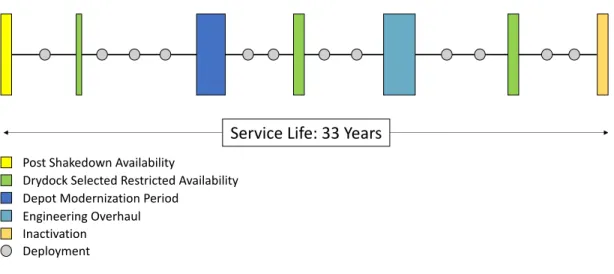
Submarine maintenance involves extensive planning, and each vessel is built with a maintenance plan already established for its entire service life. Figure 1-1 illustrates a generic life cycle maintenance plan for a submarine, where different maintenance milestones are interspersed with deployment requirements.
Although the grey dots between availabilities represent discrete deployments, time at sea is not limited to deployments alone; local operations, participation in exercises, and underway training are other important “value added” operations for submarines.
Service Life: 33 Years
Post Shakedown Availability
Drydock Selected Restricted Availability Depot Modernization Period
Engineering Overhaul Inactivation
Deployment
Figure 1-1: Generic Life Cycle Maintenance Plan for a Submarine
1.2
Availability Schedule Delays
If maintenance availabilities take longer than expected, the additional days spent in a drydock translate directly into fewer days at sea. Figure 1-2 demonstrates how successive schedule delays (depicted in red) across multiple availabilities can add up over the life of a submarine. In this example, the 12th availability is lost because of compression in the life cycle plan.
Figure 1-2: Loss of an Availability Due to Maintenance Slip
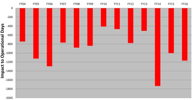
The Navy closely tracks maintenance schedule slippage because of its impact on the submarine fleet. Figure 1-3 shows the number of fleet-wide operational submarine days lost over more than a decade as a result of maintenance delays [1]. Given a pro-curement cost of $1.71 billion for each Los Angeles-class submarine1 and $2.77 billion
for each Virginia-class submarine,2 these lost operational days represent performance
which was paid for, but not realized [2][3].
Availability delays are not unique to the submarine community; the Vice Chief of Naval Operations testified before Congress that delayed maintenance periods are a fleet-wide issue with corrosive effects on warfighting readiness [4].
1The official cost is $900m in FY1990 dollars, which for the sake of comparison has been adjusted to FY2018 dollars.
-2000 -1800 -1600 -1400 -1200 -1000 -800 -600 -400 -200 0
FY04 FY05 FY06 FY07 FY08 FY09 FY10 FY11 FY12 FY13 FY14 FY15 FY16
Im pa ct to O pe ra tio na l D ays Data Date: 03/29/17
Figure 1-3: Submarine Operational Days Lost Due to Availability Overrun, Fiscal Years 2004-2016
1.3
Causes of Schedule Delays
The issue of availability delays is best summarized by the statement of VADM Thomas Moore, Commander, Naval Sea Systems Command (COMNAVSEA), to the Senate Armed Services Committee:
“The high operational tempo in the post 9/11 era combined with duced readiness funding and consistent uncertainty about when these re-duced budgets will be approved have created a large maintenance mis-match between the capacity in our public shipyards and the required work... Today, despite hiring 16,500 new workers since 2012, Naval Ship-yards are more than 2,000 people short of the capacity required to ex-ecute the projected workload, stabilize the growth in the maintenance backlog and eventually eliminate that backlog. This shortfall, coupled with reduced workforce experience levels (about 50 percent of the work-force has less than five years of experience) and shipyard productivity issues have impacted Fleet readiness through the late delivery of ships and submarines. The capacity limitations and the overall priority of work toward our Ballistic Missile Submarines (SSBNs) and Aircraft Carriers (CVN) have resulted in our Attack Submarines (SSNs) absorbing much of the burden, causing several submarine availabilities that were originally
scheduled to last between 22 and 25 months to require 45 months or more to complete.”[5]
This thesis does not purport to address operational tempo, budgeting, or manning issues; however, the need to improve availability planning and execution—by any means—is apparent.
1.4
The NAVSEA 00 Planning Summit
A month before issuing the statement quoted in Section 1.3, COMNAVSEA convened a planning summit in which stakeholders of the maintenance planning process could work together to improve availability planning and execution [6]. This Summit re-sulted in a set of 28 specific actions “to close the gaps and drive alignment between the maintenance planning budget process and the maintenance execution budgets” [7]. In particular, two of these action items serve as guideposts for the formulation of this thesis:
2. Analyze feedback mechanisms to improve identification of Growth/New Work.3
24. Review availability data and recommend appropriate upward adjustment factors to correct for known underestimation of shipyard man-day requirements caused by continued degradation when availabilities are deferred beyond class lifecycle maintenance plans.
These two items highlight the value of investigating existing shipyard data as a means to better understanding the multidimensional schedule delay problem. Analy-sis exists at the Ship Work Breakdown Structure (SWBS) level, which aggregates all systems under common umbrellas like “auxilliaries” or “hull/structure,” but it does not investigate at a finer granularity. The comparative lack of data analysis at the system level—for specific systems such as Trim or Drain—set the course for this the-sis.
3“New Work” is work that is added to an Availability Work Package (AWP) in excess of the baseline work package.
1.5
Thesis Statement
Having detailed the background and motivation for this investigation, the thesis itself is as follows:
There are specific and actionable insights which can be derived from analyzing large amounts of data at the system level across a broad cross-section of shipyard availabilities. Furthermore, a multiple linear regression model derived from that data could be used to improve the Navy’s esti-mates for New Work in future availabilities.
Chapter 2
Literature Review
U.S. Navy cost data from public shipyards is a specialized area of study; accessing the data can be problematic for academic investigations starting outside of the De-partment of Defense (DoD). Although there is a plentiful selection of defense-oriented web articles and consultant-driven publication, academic research in this field is lim-ited. This literature review found five academic works addressing shipyard cost data in the past two decades; that prior body of research helps to provide additional con-text for the problem this thesis addresses. Outside the realm of shipyard analysis, there are also many examples of the efficacy of regression analysis, which inspires the hypothesis that such methods could find value in applications with shipyard data.
2.1
Cost Analysis of Naval Availabilities
It is satisfying to the engineering mind to be able to identify the root cause of a prob-lem, to fix it, and to subsequently observe improved results—this is the quintessence of the scientific method. Because availability cost and schedule overruns are often the result of interrelated root causes, this template for a problem/solution pairing seldom obtains. Instead, high-level analysis helps to get a sense of where further attention should be directed. For instance, there are meaningful correlations between avail-ability timeliness and ship class, cost performance ratio, and work stoppages prior to work start, but little to no relationship between availability timeliness and number of concurrent availabilities, concurrence of submarine and carrier availabilities, or quan-tity or length of work stoppages [8]. Given that the implementation new shipyard performance metrics results in improved performance along those metrics over time [9], there is certainly an impetus to identify correlations of interest and then ensure that established metrics track them. Put metaphorically, we seek to find the horse’s mouth, and put the bit there.
Another approach to improving an availability’s performance is to correctly antic-ipate its duration. This is because major availabilities occur in drydocks, which are a limited resource whose allocation problem is itself worthy of study [10]. To this end, the Navy issues Technical Foundation Papers (TFPs) which prescribe the notional duration (and cost) for the various availability types. Recent work demonstrates how difficult it is for TFPs to accurately predict the true amount of work required; even when back-fed historical data, the equations used in TFPs may yield predictions far from actual results [11]. The challenge of generating accurate TFPs is also addressed in the action items from the 2017 planning summit discussed in Section 1.4, which call for the standardization and increased frequency of TFPs [7].
This thesis follows the lines of questioning of past research in that it both attempts to derive insights about the cause-and-effect relationships that steer availability per-formance, as well as to develop a more accurate predictive model for availability planning.
2.2
Applications of Multiple Regression Analysis
Although there is no historical precedent for multivariate regression analysis of ship-yard data, there is one instance of an analysis (both univariate and multivariate) for submarine operation and sustainment costs. The results of that study show that regression analysis does not provide suitable estimate cost models for predictors such as crew size, length overall, and submerged displacement [12].
Although literature referencing multiple linear regression for shipyard data is rare, there exist innumerable regression-based investigations of real-world phenomena. For example, regression analysis is extremely valuable in the field of analytical epidemi-ology [13], where regression analysis has improved understanding of the risk factors for diseases of the heart, lungs, and brain [14] [15] [16]. Other applications of mul-tiple regression analysis have led to public health insights about causal factors of bacteria blooms in lakes [17], and to economic insights about optimal gasoline taxes [18]. These examples only graze the surface of a vast body of academic investigation using regression analysis, but they are sufficient to substantiate the interest in seeing whether the same techniques could unlock benefits for availability planning also.
Chapter 3
Methodology
A chapter devoted to thesis methodology is important to both explain the metrics being used as well as their limitations. These limitations help inform the ways in which the thesis is best pursued and provide the caveats necessary to prevent data misinterpretation.
3.1
Data Source
The data used in this thesis is furnished by the Naval Sea Systems Command 04X (SEA04X) directorate. SEA04X supports the Deputy Commander for Logistics, Maintenance, and Industrial Operations and provides oversight, operation, and ad-vocacy for the Naval Shipyards. Appendix B-1 contains a figure of the organiza-tional heirarchy for the public shipyards, SEA04X, and COMNAVSEA, substantiat-ing SEA04X as the appropriate source for data in this study. Data originates from the Performance, Measurement, and Control (PMC) database, with the exception of the SSN 701 PIRA of 2009 whose data comes from the Advanced Industrial Management (AIM) database.1 In all cases, the data is queried by means of the Navy’s business
objects platform.
3.2
Basis for Data Time Interval
The selection of the timeline from December 2006 to December 2017 is premised on the publication of this thesis in June 2018 and the 2006 issuance of the “Implemen-tation of Lean Release 1.0” and “Implemen“Implemen-tation of Lean Release 2.0” memorandums
1The PMC data for this availability departs severely from all other data of its type; however, its AIM data is consistent with other completed availabilities.
from Commander, Naval Sea Systems Command. These documents issued a “...set of Corporate Improvement Initiatives and Standardization Initiatives, for standard implementation across all Naval Shipyards” [19][20]. That standardization was not immediate, and an additional Lean 3.0 memorandum further expanded Lean practices less than a year later [21]. Acknowledging that 2006 marks the beginning of a change period in availability execution (where change implies data variability that is uncor-rected), the notion of a “static” period better suited for analysis is fallacious: process improvement is an ever-continuing part of shipyard availabilities. At a minimum, all availabilities studied by this thesis are subject to the same standard of execution.
One critique of this interval selection is that the Operational Interval (OPIN-TERVAL) for Los Angeles-class submarines and the Operating Cycle (OPCYCLE) for Virginia-class submarines were both increased from 48 months to 72 months in September of 2009 [22]. This significant change to the amount of time between major availabilities implies an unmeasured bias in cost results caused by availability plan-ners adjusting to the “new normal.” To uncover any bias that may exist in availability performance due to the Lean 1.0/2.0 initiatives or to the OPINTERVAL/OPCYCLE changes, Section 5.1.2 includes a partitioned analysis of availabilities in the first half versus the second half of December 2006 to December 2017.
A final important observation is that for the time period under consideration, all four public shipyards were operating under “Mission Funding” status as opposed to the former “Navy Capital Working Fund” vehicle. The last two shipyards (Portsmouth and Norfolk) switched funding mechanisms on October 1, 2006 [23].
3.3
Availabilities Chosen for Analysis
Only availabilities which started and finished inside the specified time interval are analyzed in this thesis. The 57 availabilities examined here fall into one of five avail-ability types:
1. Depot Modernization Period (DMP)
2. Drydock Selected Restricted Availability (DSRA)
3. Extended Drydock Selected Restricted Availability (EDSRA) 4. Engineered Overhaul (EOH)2
5. Pre-Inactivation Restricted Availability (PIRA)
2The SSN 755 EOH is exempted due to the fire and untimely decommissioning of that vessel, which created an unrepresentative data set.
These availabilities can represent different durations and levels of effort; the ex-tent to which these differences might contribute to performance are investigated in Section 5.1.2. It is important to note that even between like availabilities, work on any given system can vary widely in duration and level of effort.
3.4
Metrics
There are three major cost determinants in a shipyard availability: 1. Man-Hours: This measures how long it takes to complete a job.
2. Labor Rate: This is a cost-per-hour rate which is multiplied by man-hours to obtain the cost of labor.
3. Material Cost: This is the cost of the raw goods used to build or repair system items.
This thesis only addresses the man-hours needed to complete work on a system. This metric is useful for comparison of like jobs between different shipyards because labor rates and material costs may vary according to differences in (for instance) costs of living, labor pools, day of the week, raw good shipping rate, and dollar inflation. The man-hour metric stands independent of such variables and is persistently relevant in spite of differing locations and times.
3.4.1
Leveraging Earned Value Management
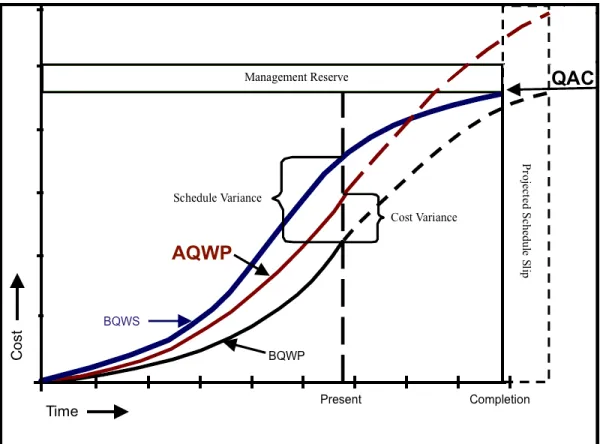
The Federal Acquisition Regulation (FAR) sets requirements for government procure-ment in the United States. The DoD (to include the Navy) must impleprocure-ment a system known as Earned Value Management (EVM) to track budgets and costs for efforts such as shipyard availabilities [24]. Figure 3-1 is a classic EVM conceptual model, with minor modifications made to suit the needs of this thesis: traditional EVM metrics refer to “cost” as opposed to “quantity” (using ACWP instead of AQWP, for instance), and some labels have been changed or removed in order to emphasize the two metrics considered in this thesis, which are Quantity at Completion (QAC) and Actual Quantity of Work Performed (AQWP).
QAC
Notionally, QAC represents an estimate made prior to starting work. It is a specific value that the entire work effort is expected to equal, once the task is complete. The
Figure 3-1: Earned Value Management Conceptual Graph
“S” shaped curve in Figure 3-1 reflects how work typically tapers at the beginning and end of a task, with maximum productivity near the midpoint, but QAC only concerns the final amount of work. It is a best-guess at the work required, and the Navy has a feedback mechanism in place whereby QAC for specific tasks gets revised based on historical data. However, estimating how many man-hours a job will require can be extremely difficult. Two jobs with the same numerical identifier can may differ in regard to the condition of the materials (for an item requiring maintenance) or to the experience of the worker.
One important characteristic of QAC is that for a completed availability (the only type considered in this thesis), the final QAC reported for a task may not be the same as the QAC which was originally estimated. This is because individual jobs can be “rebaselined,” which means that the a new, larger QAC value replaces the original value. Rebaselining has the effect of artificially improving the cost performance EVM data in an availability; however, sometimes it is necessary to rebaseline expectations for work in situations where a job’s scope was dramatically underreported. This thesis makes no effort to assess the number of rebaselines that occur for a task, and only uses the final value that existed at the time that the job was completed.
AQWP
AQWP is the other principle EVM metric considered in this thesis. It represents the final amount of work that is needed to complete a given task, after the task is complete. In Figure 3-1, AQWP is depicted as surpassing QAC, meaning that the man-hours actually required are greater than the estimate. Ideally, AQWP equals QAC at the end of a task.
As with QAC, there are some limitations to AQWP which merit discussion. AQWP is recorded after the receipt of a verbal report of job completion (or job progress) at the end of a work shift. Furthermore, one worker may report the com-pletion of several tasks over the course of a shift, leaving it to the work supervisor to determine the allocation of an eight-hour shift over the completed tasks. Database entry of AQWP is manual. The data entry does not resemble the timestamp-driven process of a shipping company; it does not generate the “pristine” data that one might desire in an analytics-driven enterprise.
3.4.2
Treatment of Anomalous Data
In the course of researching this thesis, it became apparent that bookkeeping processes exist which allow accurate reporting of man-hours at the availability level, but which can cause curious anomalies in data at the system level. For example:
1. The SSN 767 DSRA of 2009 has an AQWP transfer charge of +48,745.7 man-hours to Ship System Index (SSI) 581, and -48,745.7 man-man-hours to SSI 591. 2. The SSN 753 EOH of 2014 has an AQWP of -16,073 man-hours for SSI 043. 3. The SSN 762 DSRA of 2010, SSN 771 DSRA of 2012, SSN 776 EDSRA of 2015,
and SSN 767 DSRA of 2009 have small but negative AQWP values for SSIs 577, 000, 177, and 800, respectively.
In other cases, an numerical entry may exist for AQWP but not for QAC, or vice versa. Sometimes an SSI may have a charge of 0.0 hours for both QAC and AQWP. This thesis is not an assessment of QAC and AQWP data quality and it does not investigate or judge the causes of anomalies that exist in the data. The treatment for all cases of anomalous data is to delete them from the data set.
3.5
Tracking Work by Job Order Number
Every job in an availability is tracked with a Job Order Number, which is a 13-digit identifier used for planning and budgeting purposes. The generic format of the
alphanumeric identifier is:
12 ABC 345 67 D 89
The “345” portion of this number is known as the “Ship System Index” (SSI) and identifies the system in which work will occur for this a job. The 315 systems analyzed in this thesis are listed by SSI in Appendix A.3; only these three digits are used to uniquely identify man-hour data throughout this thesis. This means that no inferences can be made about subcomponents of systems; instead, all subcomponent data is aggregated by SSI into two sum totals (QAC and AQWP) per system. One availability may have work in anwhere from 80-200 systems, depending on the duration and scope of the availability. Furthermore, one unique system may get maintained in two different availabilities, yet have dramatically different man-hour expenditures based on the unique states of that system. Because of this inherent variability, it is difficult to make quantitative statements about maintenance at the system level using some fixed performance metric. Instead, this thesis reframes the problem as an investigation into the Navy’s ability to estimate man-hours for a task. While cross-availability performance measurement is stymied by the high degree of variability at the system level, the broader question of estimate validity adjusts with the scope of work. Thus the first objective in the thesis statement, which is intentionally vague to allow for exploration based on the constraints of available data, gains focus as a targeted investigation of estimate accuracy.
3.6
Population Observations: Eliminating Outliers
The data structure created in this thesis is a 315x57 matrix, given the 315 systems maintained across 57 availabilities. In a 315x57 matrix, there are 17,955 cells, but only 7,016 cells have cost data in them; all of the remaining cells of this matrix are not-a-number or “NaN” values. Given the QAC and AQWP anomalies addressed above, the question arises as to whether all 7,016 data entries are “believable” or otherwise grounded in reality. One way to populate the 315x57 matrix is by placing the quotient of AQWP/QAC in applicable cells and then observing trends. Section 4.1 details use of the ratio AQWP/QAC as a method for data analysis, but here we will briefly consider the methodological validity of this tool.
Of the 7,016 maintained systems, 477 entries of AQWP/QAC are larger than two, implying that the actual work required was at least double the amount predicted in the estimate. For those 477 entries, the mean is 42.7 and the standard deviation is 274.8.
For the remaining 6,539 system values (all of which fall between zero and two), the mean is 1.07 and the standard deviation is .35.
The data characteristics of the latter group are of great interest because they so closely approximate a normal, or Gaussian, distribution. The vast majority of the data is compact and consistent, while a small subset is extreme and variable. The assumption made in this thesis is that the values in that small and variable subset of data—477 out of 7,016 entries—can be rejected because either:
1. They are caused by data anomalies, or
2. They are caused by very small QAC values that divide into large AQWPs, demonstrating more about small number division than about the Navy’s ability to generate reasonable estimates.
When the maximum quotient in the entire set is 3,142.7, there is a clear impetus to delete that value because it so clearly breaks the meaning inherent to the quotient comparison. And if this value is to be deleted, then perhaps too the next maximum, which is 2,860.7. And the next maximum of 2,656... Rather than wrestle with where to draw the cutoff line for aberrant data values, we instead prefer to select a value for its conceptual merits; in this case, “anything larger than two” is a good choice for exemption from the data set based on mean and standard deviation characteristics. This is not to say that there is nothing to be learned from those specific individual outliers; to the contrary, many shipyard representatives have the uncanny forensic ability to recreate the chain of events that resulted in a specific value. However, this thesis seeks broad inferences that apply to all availabilities rather than insights from case studies of outliers.
3.7
Regression Data
The second portion of this thesis explores the potential use of multiple linear regression to improve QAC estimates. This implies that the error inherent to QAC is eliminable and that large amounts of data can yield a predictive model which reduces that error. Whether or not this is true, an ill-conceived regression model will yield a useless result.
To build a good regression model, we must first recognize the relationships which exist within the data. QAC is intended to predict AQWP—this implies that the independent variable matrix must be comprised of QAC values and the dependent “solution” matrix contains AQWP values. However, there are also important rela-tional qualities within QAC data that inform the model. All SSIs in the 000- and
900-series, as well as two specific 800-series, are contingent on the the work expected for systems 100-800. Therefore, a one-way dependency relationship exists within the data; additional 100 series work can result in a corresponding increase in 000 and 900, but not the other way around. Therefore the regression model omits 000, 900, and two of 800 series SSIs, instead investigating the QAC-to-AQWP relationship expressed by the remainder of the SSIs.
Section 3.6 explicitly addresses the treatment of anomalous data; the regression-based portion of this thesis also resolves the problem of anomalous data, albeit im-plicitly. First, the regression models use direct man-hour data (no division or other adulteration), eliminating the possibility of dividing by very small numbers to create inflated values in the data. Second, the regression models exempt any SSI with fewer than 14 observations, and in many cases exempted even more SSIs depending on the need to generate a meaningful set of coefficients.3 Due to the fact that regression models are more meaningful when derived from many observations (rather than very few), this thesis employed a “pruning” process to arrive at the largest set of nonzero regression coefficients. This method is discussed in Section 4.2.1, and the result of this method is that it removes underrepresented SSIs from the model until there is enough fidelity in the data to generate a set of nonzero coefficients and their asso-ciated regression statistics. This ensures that anomalies are either eliminated from consideration, or they are aggregated with other data of the exact same SSI which results in a smoother data profile.
3SSIs with very little representation amongst the data drive the family of regression coefficients to zero, resulting in a model with no predictive power.
Chapter 4
Methods
There are two primary methods, or tools, used to test this thesis: the first is a high-level observation of the total population of availabilities; the second is the creation of two multiple regression models based on the same set of data. This chapter de-tails the steps taken to create these tools, with the intent that this research can be independently reproduced and verified.
4.1
Population Observations
To make meaningful observations about the characteristics of submarine availability data, it first helps to consider what we expect to see in a process that produces a random result. Given the metrics QAC and AQWP discussed in Section 3.4.1, we expect that if a work estimate perfectly anticipates the work required, then 𝑄𝐴𝐶 = 𝐴𝑄𝑊 𝑃 , and subsequently:
𝐴𝑄𝑊 𝑃 𝑄𝐴𝐶 = 1
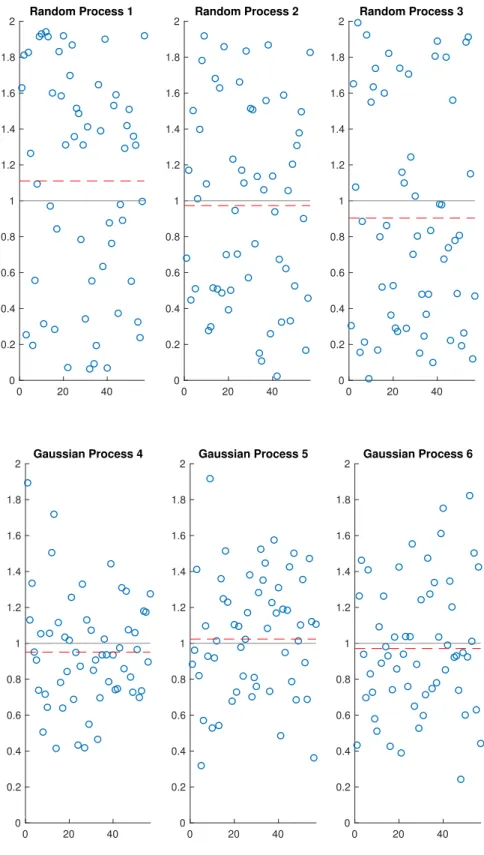
Using this baseline, we want to build an intuition about the extent to which a process creates quotients which are less than one (overestimates) or greater than one (underestimates). Given that this thesis studies 57 availabilities whose work estimate quotients fall predominantly near one, the plots in Figure 4-1 show 57 points randomly distributed between zero and two, as a baseline for our intuition.
Note that the dashed line illustrates the mean for each data set. As this is an intuition-building exercise, the specific values of this data aren’t as important as the general impressions that the visual plots create. Plots 1,2, and 3 in Figure 4-1 show randomly distributed points in the range [0,2], but we don’t necessarily expect that work estimates will be random. To the contrary, Section 3.6 demonstrates that they
0 20 40 0 0.2 0.4 0.6 0.8 1 1.2 1.4 1.6 1.8 2 Random Process 1 0 20 40 0 0.2 0.4 0.6 0.8 1 1.2 1.4 1.6 1.8 2 Random Process 2 0 20 40 0 0.2 0.4 0.6 0.8 1 1.2 1.4 1.6 1.8 2 Random Process 3 0 20 40 0 0.2 0.4 0.6 0.8 1 1.2 1.4 1.6 1.8 2 Gaussian Process 4 0 20 40 0 0.2 0.4 0.6 0.8 1 1.2 1.4 1.6 1.8 2 Gaussian Process 5 0 20 40 0 0.2 0.4 0.6 0.8 1 1.2 1.4 1.6 1.8 2 Gaussian Process 6
are very nearly Gaussian. Plots 4, 5, and 6 of Figure 4-1 show data generated with a Gaussian mean (𝜇) of 1 and standard deviation (𝜎) of 1/3, which is very similar to our data and is centered on the range [0,2] to maintain consistency. The visual differences between plots 1-3 and 4-6 are immediately apparent, with Gaussian distributions being "clustered" around one and becoming less prevalent at the extremes of the range. Note that this is entirely by design; the Gaussian Process charts could be made to resemble the random process charts or even to display nothing (on the range [0,2]) by selecting different values of 𝜇 and 𝜎. However, such graphs would do nothing to build our intuition as they wouldn’t resemble man-hour estimate data.
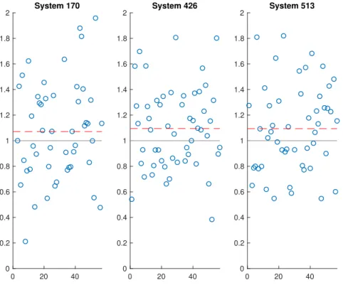
Next we consider the case of actual systems which exhibit the kind of charac-teristics we expect from a Gaussian distribution. Figure 4-2 shows three different submarine systems—170, 426, and 513—which exhibit the kind of quotient distribu-tion that we now expect. Note in particular that a nontrivial number of quotients fall below and above 1; this confirms the Gaussian tendency to generate comparable numbers of over- and underestimates.
0 20 40 0 0.2 0.4 0.6 0.8 1 1.2 1.4 1.6 1.8 2 System 170 0 20 40 0 0.2 0.4 0.6 0.8 1 1.2 1.4 1.6 1.8 2 System 426 0 20 40 0 0.2 0.4 0.6 0.8 1 1.2 1.4 1.6 1.8 2 System 513
Figure 4-2: Actual Data for Three Submarine Systems
Now that a standard of normalcy is established, we ask what would constitute abberant or “interesting” data. To answer this, we must revisit the premise of this conceptual framework; namely, that the quotient of one represents an estimate that
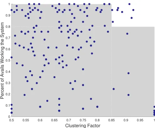
exactly matched the actual work that was later required. Given that we can look at the estimates for systems over many availabilities, we are primarily interested in whether we consistently overestimate or underestimate work for a given system, in spite of a range of differences such as shipyard, availability type, etc. In other words, we want to know if a disproportionate number of quotients is greater (or less) than one. Figure 4-3 shows a scatterplot of the 315 systems, where each system is plotted according to two pieces of information:
1. Percentage of Availabilities Working the System: This counts the number of times the system was worked and divides it by the total number of availabilities considered (57). This helps us to rule out systems which do not have sufficient representation in our data set to merit strong conclusions.
2. Clustering Factor (CF): Consider the number of availabilities where a system’s quotient is less than one, and divide by the number of availabilities (57). Due to symmetry, one minus this number equals the the percentage of systems with quotients greater than one; the CF counts only the largest of these two values such that the range is [0.5,1]. This value represents the extent to which system estimates are “lopsided;” if there is an equal number of over- and underestimates, the CF will equal 0.5, and if they are either all below one or all above one, the CF will equal 1.
Points existing in the top right of this plot have both a high degree of representa-tion across all availabilities, as well as very densely clustered quotients either above or below one. Using an 80% representation rate and a CF of .85, we see that nine systems meet these criteria and constitute an excellent starting point for investigating submarine availability performance. In this thesis, systems meeting the above spec-ified critera for representation and clustering are referred to as consistently poorly estimated systems. All such systems are addressed in Chapter 5.
0.5 0.55 0.6 0.65 0.7 0.75 0.8 0.85 0.9 0.95 1 Clustering Factor 0 0.1 0.2 0.3 0.4 0.5 0.6 0.7 0.8 0.9 1
Percent of Avails Working the System
Figure 4-3: Selecting the Most “Interesting” Systems
4.2
Regression Analysis
The second method to test this thesis is a multiple regression analysis to predict New Work. A multiple regression model attempts to characterize the relationship between independent variables (systems worked) and one dependent variable (avail-ability cost). In the context of this thesis, a successful regression model would more accurately predict AQWP for New Work than QAC. As addressed at length in Sec-tion 3.7, the model would noSec-tionally “back out” the error inherent to QAC to provide a more accurate estimate of how much work a new job will require. Therefore the hypothesis being tested is that each independent variable (expressed as QAC) has a predictive relationship with the resulting AQWP.
To test a model’s ability to predict New Work, it is necessary to have documen-tation of the New Work that occurred in an availability, expressed both in QAC and AQWP. Only 29 availabilities between PHNS and PSNS meet this requirement; these availabilities are explicitly identified in Appendix A.2. Whereas the population ob-servations in Section 4.1 concern a quotient, the regression models use the man-hour values of QAC and AQWP, with one minor modification: all the New Work QAC and AQWP is subtracted from the data. The intent of this is that it preserves the
maxi-mum number of availabilities to create the best-quality regression possible, while still providing fresh data that can be used to assess the model’s efficacy. Furthermore, the ability to accurately estimate the impact of New Work on an availability is of great interest to the Navy.
Each availability constitutes an “observation” of work; more specifically, each one constitutes a family of observations on estimate/actual cost pairs for specific systems. No single availability maintains all 315 systems, and very few systems are represented in every availability. Attempting to generate a regression model for 315 independent variables with only 57 observations is not possible. Formulated mathematically, there are more variables than equations to solve for them; the system is indeterminate. However, there are two straightforward ways of reducing the number of variables: the first is to segment the availability data by SSIs; the second, to segment it by SWBS groups. In each case, the goal is to produce a set of regression coefficients which each multiply with an associated independent variable (QAC) and then sum to estimate revised AQWP. A generic model for such a relationship is:
𝐴𝑄𝑊 𝑃𝑟𝑒𝑣 = 𝑓 (𝑄𝐴𝐶)
More specifically, for each i𝑡ℎ QAC value, the model will propose a corresponding
coefficient 𝜆𝑖; the sum of the products of these pairings is the revised estimate for
AQWP:1
𝐴𝑄𝑊 𝑃𝑟𝑒𝑣 =
∑︁
𝜆𝑖* 𝑄𝐴𝐶𝑖
4.2.1
Regression by SSI
The original aproach for this thesis was conceived as a summation of all QAC data and all AQWP data in order to obtain a regression model, but because the system has too many variables, that approach is not valid. However, the availability cost data is granular enough that it can be segmented into subcategories to reduce the number of variables while maintaining the number of observations at 57. Instead of one massive 57x315 multiple regression model, eight smaller models can be constructed by selecting estimates for smaller batches of systems (informed by SWBS group) and by using the AQWP obtained only for those systems across all 57 availabilities. Figure 4-4 shows a miniaturized version of the 57x315 matrix developed for this research, with
1Note that the i values correspond to three digit numbers that do not increase linearly and therefore do not lend themselves to a convenient summation notation starting with i = 1 and proceeding to n.
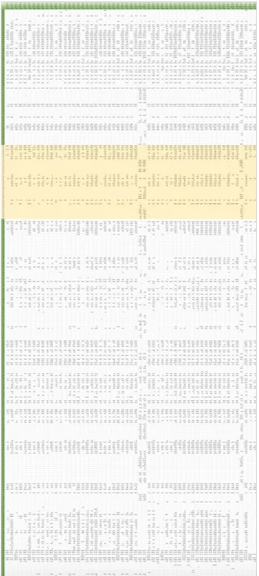
all of the SWBS 200 SSIs highlighted.2 This highlighted section, along with the corresponding AQWPs, results in a 57x41 matrix which is solvable. Repeating this method for the remaining seven SWBS groups breaks the data into smaller pieces that can be solved piecemeal.
This solution is not without problems—some systems have little representation across the 57 availabilities (this characteristic is evidenced by the horizontal white bands of empty cells in Figure 4-4). Creating a regression model with so much missing data most often results in coefficient matrices comprised entirely of zeroes. Given that a model built from many data points is more valuable than one built with few, the first step is to delete those SSIs with relatively low representation. This “pruning” process begins by deleting all systems with 14 or fewer observations. Even after doing this for each SWBS category, the derived regression coefficients have many zeroes. This poses a twofold problem:
1. The regression model produces too many zero-value coefficients, which serve no purpose in a predictive model because they eliminate (rather than scale) a baseline estimate. Therefore, systems must be removed from the model to improve its predictive power.
2. When it is time to validate this model using New Work data, deleted systems will find no expression in the model. If there is a New Work item for which there is no corresponding coefficient, this constitutes a missed opportunity to provide an improved estimate.
The solution pursued in this thesis is to iteratively observe which systems have a zero coefficient, find the one with the fewest number of observations, delete it, and re-run the regression model for the remaining systems until there are no zero-value coefficients. Chapter 5 discusses the results obtained by using the MATLAB “fitlm” function to generate the regression models.
4.2.2
Regression by SWBS
Creating a multiple regression model using SWBS groups is straightforward compared to the SSI method. As before, all New Work values are first subtracted from AQWP and QAC. This secures a testable set of New Work data which can be used to evaluate the regression model. Then, all QAC values are summed according to their first digit;
2The matrix displayed is actually 315x57, with SSIs as rows and availabilities as columns, but all data was transposed prior to regression. This figure is not scalable and is only intended to help readers understand the method.
for instance, the estimates for systems 111, 112, 117, ... 191 are all summed into the “100” group. Once this is complete for each of the 57 availabilities, and for SWBS 100-800, we have an 8x57 matrix of QAC values aggregated by SWBS group, and a corresponding 8x1 matrix of AQWP values. Using the “fitlm” function in MATLAB, we can generate eight regression coefficients which correspond to each SWBS group. Finally, we multiply each New Work item (from one the 29 applicable availabilities) by the corresponding coefficient to produce a revised estimate. Summing these revised estimates permits direct comparison to the actual hours attained (AQWP); Chapter 5 discusses these results.
Chapter 5
Results
5.1
Population Observations
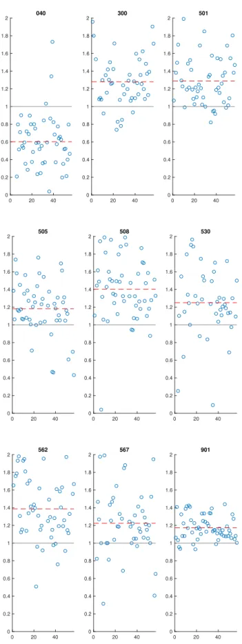
There are nine systems across 57 availabilities for which there is consistent inaccuracy in estimating the scope of work. These consistently poorly estimated systems are:
040 300 501 505 508 530 562 567 501
Plotting these systems about the target mean of 1 on the range [0,2] is particularly interesting, given the time we spent building our intuition in Section 4.1. Figure 5-1 shows these results. Note the extreme amount of clustering, whereby quotients fall predominantly above 1 (with the exception of system 040, whose quotients are predominantly below 1), indicating a consistent underestimation of work for these systems.
5.1.1
Prioritizing Error Severity by System
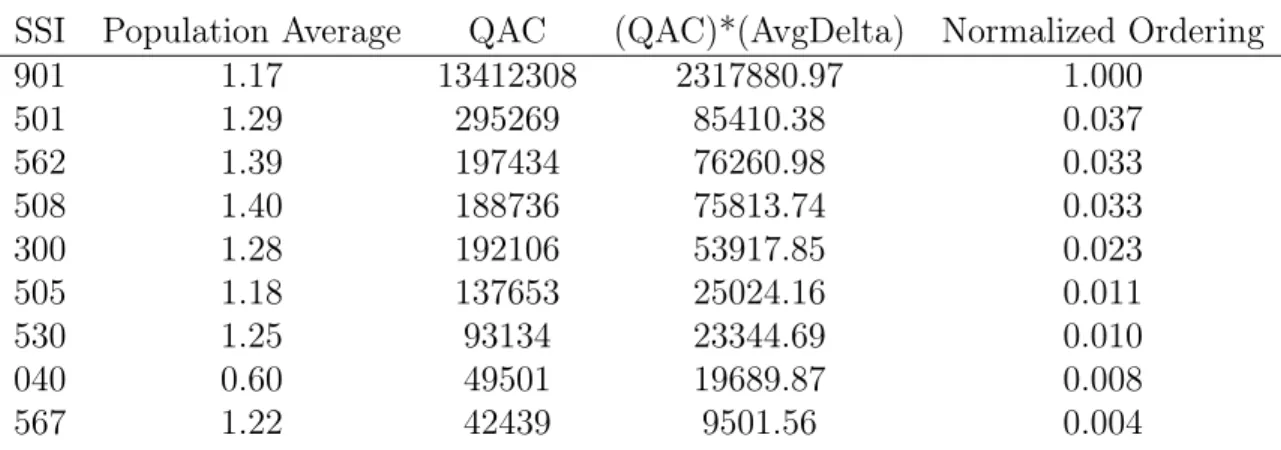
In order to prioritize where future attention should be placed, is important to iden-tify the precedence ranking of these estimates. First, a precedence ranking must incorporate the severity of the over- or underestimate. To do this, we find the mean estimate error for a system. This is graphically represented by the distance between one and the dashed lines in Figure 5-1. Second, a precedence ranking must include QAC, which captures the magnitude of work which can be directly compared to other systems’ QAC values. By normalizing the multiple of mean estimate error and QAC, we can examine a tier ranking of problematic systems. Table 5.1 traceably shows how to derive the priority ranking for the nine systems of interest.1
0 20 40 0 0.2 0.4 0.6 0.8 1 1.2 1.4 1.6 1.8 2 040 0 20 40 0 0.2 0.4 0.6 0.8 1 1.2 1.4 1.6 1.8 2 300 0 20 40 0 0.2 0.4 0.6 0.8 1 1.2 1.4 1.6 1.8 2 501 0 20 40 0 0.2 0.4 0.6 0.8 1 1.2 1.4 1.6 1.8 2 505 0 20 40 0 0.2 0.4 0.6 0.8 1 1.2 1.4 1.6 1.8 2 508 0 20 40 0 0.2 0.4 0.6 0.8 1 1.2 1.4 1.6 1.8 2 530 0 20 40 0 0.2 0.4 0.6 0.8 1 1.2 1.4 1.6 1.8 2 562 0 20 40 0 0.2 0.4 0.6 0.8 1 1.2 1.4 1.6 1.8 2 567 0 20 40 0 0.2 0.4 0.6 0.8 1 1.2 1.4 1.6 1.8 2 901
Note that system 901 dominates the other systems due to its relatively large QAC. This is consistent across all projects and is caused because system 901 tracks project management overhead for every availability; it is always present and is always significant. We might consider excluding system 901 (and other similar SSIs) because it is not true “wrench turning” work on a system, but it nevertheless meets the criteria of consistently poor estimation, and constitutes an interesting insight.
SSI Population Average QAC (QAC)*(AvgDelta) Normalized Ordering
901 1.17 13412308 2317880.97 1.000 501 1.29 295269 85410.38 0.037 562 1.39 197434 76260.98 0.033 508 1.40 188736 75813.74 0.033 300 1.28 192106 53917.85 0.023 505 1.18 137653 25024.16 0.011 530 1.25 93134 23344.69 0.010 040 0.60 49501 19689.87 0.008 567 1.22 42439 9501.56 0.004
Table 5.1: Ranking Method for Systems with Poor Estimates
5.1.2
Using Subsets of the Data to Gain Insight
Another interesting question is how subsections of the data (availability type, ship class, shipyard, and time period) compare to the aggregate. Having identified the nine systems in Table 5.1, we ask how the family of consistently poorly estimated systems changes depending on the “slice” of the data we observe. Note that the criteria for consistently poor estimation remains the same: a system must have been worked in at least 80% of the availabilities considered, and the system’s CF must be greater than or equal to 0.85. Because these thresholds assess an integer divisor and dividend, the number of poorly estimated systems that meet or exceed the thresholds is subject to “inflation.”
This scenario is best interpreted as a classic “coin flip” question, where the like-lihood of attaining an AQWP/QAC quotient greater than one is 50%, and the al-ternative (a quotient less than one) is also 50%.2 Consider an example evaluating
the CF threshold of 85%. Using Depot Modernization Periods, which represent only four availaibilities, all four must fall either above or below one, because 3/4 is 75%
2This is not exactly accurate, since AQWP/QAC can also equal one, but there exist only 100 quotients equal to one out of the 7,016 systems worked, so this analogy is sufficient for the qualitative conclusions derived.
which fails to meet the CF threshold. In a random process, the chance of getting 4/4 “heads” flips is equal to 0.0625. If we consider the aggregate data set, we need 49/57 (or more) “heads” flips—quotients above one—to satisfy the CF threshold. This has a far lower probability of 1.3584e−8. This simple example illustrates the bias that small sample sizes have towards false positives; furthermore, this effect becomes more pronounced as the observed pool of availabilities shrinks. For the analysis below, data subsets of 10 or fewer are dismissed as too small to be meaningful.
1. Availability Type
DMP: The data contains only four Depot Modernization Periods, which is too small for a meaningful comparison to the aggregate.
DSRA: The data contains 24 Drydock Selected Restricted Availabilities yielding seven systems of interest, which is comparable to the aggregate.
EDSRA: The data contains only four examples of Extended Drydock Se-lected Restricted Availabilities, which is too small for a meaningful comparison to the aggregate.
EOH: There were 14 Engineered Overhauls, and these feature 44 flagged systems. This is a surprisingly high number, even accounting for inflation. This suggests that a disproportionately high number of poor estimates exist in EOHs. PIRA: There were 11 Pre-Inactivation Restricted Availabilities in the data with 12 flagged systems. This is comparable to the aggregate.
2. Submarine Class
Los Angeles (688): The vast majority (54) of submarines examined in this thesis were Los Angeles-class submarines. Of interest is the fact that remov-ing Virginia-class submarines added one additional system of concern to the aggregate nine, for a total of 10 flagged systems.
Virginia (774): Only three Virginia-class submarines existed in this study (comprising three of the four EDSRAs). No meaningful insights can be derived from this subset.
3. Shipyard
NNSY: Norfolk Naval Shipyard had six availabilities, which is too small for a meaningful comparison to the nine systems from the aggregate.
PHNS: Pearl Harbor Naval Shipyard conducted 26 availabilites, which is more than any of the other shipyards. The number of systems which meet the
criteria for consistently poor estimation is 18, which is double the amount for the aggregated data. This suggests that a disproportionately high number of poor estimates exist at PHNS.
PNSY: Portsmouth Naval Shipyard followed a close second to PHNS with 22 availabilities, yet the number of systems which flag is only 13. This amount is reasonably close to the aggregate 9, taking quotient inflation into account.
PSNS: Puget Sound Naval Shipyard had three availabilities, which is too small for a meaningful comparison to the aggregate.
4. Time Period
2006-2011: The first half of the analyzed timeline has 34 availabilities with eight flagged systems, which is comparable to the aggregate.
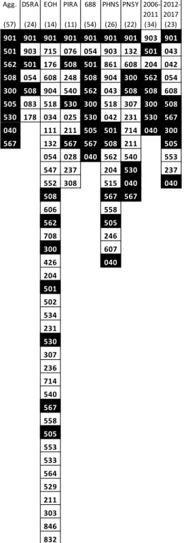
2012-2017: The remaining 23 availabilities are captured in the second half of the timeline, with 12 flagged systems. This is comparable to the aggregate. Figure 5-2 condenses the above information into a comparative visual. For the aggregated data, it depicts the nine consistently poorly estimated systems in black; it also depicts those same systems in black wherever they appear in smaller data partitions. Beneath the identifier for each column is a number in parenthesis which corresponds to the number of availabilities contained in that partition. All systems are ranked from highest- to lowest-priority for future investigation, consistent with the example in Section 5.1.1. This visual gives a sense of the work estimation problem considered from many different perspectives. One interesting observation of the raw data used to compile this thesis is that PHNS conducted 3/14 of the EOHs, while PNSY conducted 9/14 EOHs; this suggests that PHNS estimates are not being domi-nated by a disproportionate assignment of EOHs. Another worthwhile observation is that the Lean 1.0/2.0 initiatives and the OPINTERVAL/OPCYCLE changes do not result in significant differences in the number of erroneous estimates, as compared to the aggregate, over time.
Agg. (57) DSRA (24) EOH (14) PIRA (11) 688 (54) PHNS (26) PNSY (22) 2006-2011 (34) 2012-2017 (23) 901 901 901 901 901 901 901 903 901 501 903 715 076 054 903 132 501 043 562 501 176 508 501 861 608 204 042 508 054 608 248 508 904 300 562 054 300 508 904 540 562 043 508 508 608 505 083 518 530 300 518 307 300 508 530 178 034 025 530 042 231 530 567 040 111 211 505 501 714 040 300 567 132 567 567 508 211 505 054 028 040 562 540 553 547 237 204 530 237 552 308 515 040 040 508 567 567 606 558 562 505 708 246 300 607 426 040 204 501 502 534 231 530 307 236 714 540 567 558 505 553 533 564 529 211 303 846 832 435 040 440
5.2
Regression Analysis
5.2.1
Regression by SSI
The method described in Section 4.2.1 yields the set of regression statistics found in Appendices A.4 through A.11, which includes the regression coefficients. Those 88 coefficients comprise the following regression model by SSI:
𝐴𝑄𝑊 𝑃 |𝑆𝑆𝐼 =∑︁𝜆𝑖* 𝑄𝐴𝐶𝑖
Expanding the model slightly for the benefit of the reader, the model is as follows: 𝐴𝑄𝑊 𝑃 |𝑆𝑆𝐼 = 𝜆111* 𝑄𝐴𝐶111+ 𝜆131* 𝑄𝐴𝐶131+ ...𝜆847* 𝑄𝐴𝐶847
This model is applied to New Work QAC, where applicable, to create a revised estimate for the impact of New Work on an availability. For New Work which has no associated regression coefficient, the QAC value is left as-is to be summed with the revised AQWP numbers (the premise is that this model will be agnostic to QAC values which have no representation in the predictive model). The regression statistics themselves merit a brief discussion, if for no other reason than to address the fact that so many p-values are “large,” or at least larger than 0.05. Typically when a p-value passes that threshold, it implies that the associated regression coefficient is not statistically relevant, and that a random data set may have produced a similar coefficient. This implies that for a coefficient with a high p-value, the hypothesis in Section 4.2—that QAC has a predictive relationship with the resulting AQWP—is false. Very small p-values are indeed desireable, and it is possible that eliminating more SSIs from each “family” of models would improve the regression model. However, as addressed in Section 4.2.1, there is tension between models that have nice statistical properties and those that have enough fidelity to be of useful predictive value. In other words, removing SSIs may improve the model’s statistics but neuter its ability to predict anything. As for the R2 values, they are generally high or very high, which is desireable for predictive models, but is not a standalone metric for model suitability. The percent error inherent to the original estimate and to the revised (regression-based) estimate can be directly compared to evaluate which estimate is better. Fig-ure 5-3 shows the relative percent errors between the two types of estimates.
The results show that a regression model derived from SSIs does not anticipate actual work better than QAC in any of the 29 availabilities. Furthermore, in most cases the estimate is much worse than unadulterated QAC.
698 FY10 DSRA698 FY14 DSRA699 FY11 DSRA701 FY09 PIRA705 FY11 PIRA711 FY07 EDSRA713 FY08 DSRA713 FY12 PIRA715 FY09 DSRA715 FY13 PIRA717 FY15 DSRA721 FY10 EOH722 FY08 DSRA722 FY10 EOH724 FY13 DSRA758 FY07 DSRA758 FY14 EOH759 FY08 DSRA762 FY10 DSRA763 FY12 DSRA766 FY11 DSRA770 FY14 DSRA771 FY07 DMP771 FY12 DSRA772 FY15 DSRA773 FY08 DMP773 FY13 DSRA775 FY12 EDSRA776 FY15 EDSRA
Availabilities with Testable New Work Data
0 50 100 150 200 250 300 350 400
Predictive Model Percent Error
Regression Traditional
Figure 5-3: New Work Estimates Derived from a SSI Regression Model
5.2.2
Regression by SWBS
The method described in Section 4.2.2 yielded a different set of regression coefficients (and associated statistics) for the eight SWBS groups. Because this set of informa-tion is much shorter than that produced by the SSI-based model, the informainforma-tion is included here for convenience:
SWBS Group Coefficient 𝜆𝑖 Std Error t-Stat p-Value R2
(Intercept) -97613 25675 -3.8018 0.00042959 0.97 100 2.5554 0.22641 11.287 1.0264e-14 200 0.97487 0.8411 1.159 0.25256 300 7.8171 1.9598 3.9888 0.00024157 400 1.3346 0.43607 3.0606 0.0037173 500 2.0305 0.46506 4.3661 7.3306e-05 600 -3.5105 0.97948 -3.5841 0.0008277 700 -0.86144 1.5999 -0.53843 0.59293 800 1.6503 0.25295 6.5241 5.1912e-08
Applying these coefficients to the cumulative QACs by SWBS yields a revised work estimate as expressed by the following regression model:
𝐴𝑄𝑊 𝑃 |𝑆𝑊 𝐵𝑆 =∑︁𝜆𝑖* 𝑄𝐴𝐶𝑖
A slightly expanded model (to aid in comprehension) is as follows: 𝐴𝑄𝑊 𝑃 |𝑆𝑊 𝐵𝑆 = 𝜆100* 𝑄𝐴𝐶100+ 𝜆200* 𝑄𝐴𝐶200+ ...𝜆800* 𝑄𝐴𝐶800
Both the original QAC and the revised, regression-based estimate can be directly compared to AQWP to derive respective error factors. Before looking at the plotted results, we note that the p-values of SWBS coefficients 200 and 700 are much higher than 0.05, indicating that randomly generated data may just as easily have produced the associated coefficients; however, the remaining coefficients all have very small p-values which suggests that they are highly statistically significant. Notionally, all of the p-values would express statistical significance, but at a minimum, this model appears to be better than anything produced under the SSI approach. Finally, the R2 of 0.97 could mean that the model has good fit and that it has has high predictive
power. Figure 5-4 shows the relative errors between the two types of estimates.
698 FY10 DSRA698 FY14 DSRA699 FY11 DSRA701 FY09 PIRA705 FY11 PIRA711 FY07 EDSRA713 FY08 DSRA713 FY12 PIRA715 FY09 DSRA715 FY13 PIRA717 FY15 DSRA721 FY10 EOH722 FY08 DSRA722 FY10 EOH724 FY13 DSRA758 FY07 DSRA758 FY14 EOH759 FY08 DSRA762 FY10 DSRA763 FY12 DSRA766 FY11 DSRA770 FY14 DSRA771 FY07 DMP771 FY12 DSRA772 FY15 DSRA773 FY08 DMP773 FY13 DSRA775 FY12 EDSRA776 FY15 EDSRA
Availabilities with Testable New Work Data
0 50 100 150 200 250 300
Predictive Model Percent Error
Regression Traditional
Figure 5-4: New Work Estimates Derived from a SWBS Regression Model The results show that a regression model derived from SWBS groups anticipates actual work better than QAC in only one out of 29 availabilities. The margin of
improvement for that one availability is small; in all remaining instances, the margin by which the model is worse than QAC is substantial.
5.2.3
Understanding the Regression Results
Regression by SSI and by SWBS clearly fail to produce better estimates. During the course of this research, there arose several considerations that complicate the use of multiple linear regression for shipyard man-hour data. The following constraints explain why the regression models perform so poorly.
Observational Data is Asymmetric and Sparse
This study included 57 total availabilities, and no availability includes work for every one of the 315 systems considered in this thesis. Therefore, at the system level, the true number of observations was less than 57 most of the time. The typical range of observations for system data is between 35 and 57. The nonstandard number of observations at the system level is an unavoidable real-world constraint which has an adverse effect on the quality of regression analysis. This contrasts with the epidemiological studies cited as inspiration for this study; for instance, in determining factors that contribute to an algae bloom, one has access to pH, temperature, salinity, etc., with every single measurement. It cannot be overstated that the “holes” existing in shipyard cost data represent a different kind of data set than that which is produced from the sampling of lake water.
New Work is Asymmetric
One would expect that the regression coefficient for each SSI would be somewhat near one, perhaps a bit higher or a bit lower, such that work estimates are compressed or expanded slightly to arrive at a better estimate—this would be consistent with the goal of “backing out” any error inherent to a QAC estimate. Inspection of the regres-sion coefficients in Appendices A.4 through A.11 rebuts this expectation thoroughly, as many coefficients are negative, and there exist many with magnitudes exceeding 5, 10 or even 20. For a population of New Work that includes every regressed variable, each variable’s coefficient maps to a line of best fit derived from all variables. How-ever, real-world availabilities typically do not have New Work in all possible SSIs. To the contrary, New Work is unevenly distributed depending on the material condition of the submarine. Consider the hypothetical case of a New Work estimate for system 178, with no other New Work for 100-series SSIs (the family of SSIs whose coeffi-cients are derived with, and innately tied to, system 178’s coefficient). The estimate
would be multiplied by -5.6878, and it would be severely imbalanced because of the lack of other series 100 SSIs. This process would then be repeated for the sundry of New Work items across SSIs in SWBS 200, 300, etc. The resulting estimate becomes a Frankenstein of unmatched, standalone regression coefficients which do not enjoy the “best fit” contributions of the other related coefficients in each respective SWBS family. This same kind of imbalance occurs in SWBS-derived regression estimates (which have only eight coefficients rather than 88), and is reflected in Figures 5-3 and 5-4, where regression-derived estimates are grossly more erroneous than unadulter-ated QAC. This issue would persist even if the regression models had used fewer SSIs to obtain “statistically pleasing” p-values (a critique acknowledged in Section 5.2.1). Models Are Too Generic
This thesis did not investigate specialized regression models developed according to the subsets explored in Section 5.1.2. It is possible that coefficients of better fit could be attained by constraining the data set by availability type, shipyard, etc. The drawback to this method is that some of the subsets are too small to generate nonzero regression coefficients.
Models Are Overfit
The high R2 values represented in the regression statistics could conceivably imply
that the regression model is a good fit and has high predictive power; however, Fig-ures 5-3 and 5-4 clearly show that the models have poor predictive power. As a result, the high R2 indicates an overfit model which has too many predictor
vari-ables. Differently formulated regression problems would remove variables to improve the predictive power of the model, but doing that would not be meaningful in the context of this problem statement. For instance, a predictive model which is agnostic to inputs from SWBS 700 is of little value when New Work must occur in this group.
Chapter 6
Conclusions and Future Work
There are specific and actionable insights which can be derived from analyzing large amounts of data at the system level across a broad cross-section of shipyard availabilities...
This objective was highly successful. Section 5.1 defines and ranks specific systems with consistently poor estimates. Furthermore, it also partitions the data in order to gain insights about what drives these estimates to be consistently poor. Although the SSI identification codes are never mapped to their respective systems in this thesis, discussions with individuals who have worked in this field extensively have confirmed that these systems correspond with the ship maintenance community’s “tribal knowledge” of which systems are notoriously difficult. This thesis provides a quantitative substantiation of that tribal knowledge, and enhances it with a priority ranking that directs future work. An excellent path for follow-on research would be to repeat this type of analysis at the subsystem level for the nine systems identified in Section 5.1. This could determine whether individual components are driving the consistently poor estimates for the entire system.
...Furthermore, a multiple linear regression model derived from that data could be used to improve the Navy’s estimates for New Work in future availabilities.
Unfortunately, this objective was unsuccessful. It would have been a fantastic breakthrough to be able to provide the Navy with a process for improving New Work estimates, but insights gained while attempting to do this affirm the unsuitability of linear regression as a predictive tool for availability cost. The high degree of variability inherent to a specific availability implies the need for a flexible tool, and it may simply be that multipler linear regression is not the right tool for “solving” the
complexity of availability planning and execution. Future work in this area includes multiple linear regression of smaller, more coherent subsections of the data (such as a regression model for only one availability type), nonlinear regression models, or perhaps an investigation into the suitability of more advanced modeling techniques such as neural networks.
In addition to the value of a better estimation model for availabilities, a ma-jor concern that emerged during the course of this research is that of data quality. Compared to major public companies in the United States, the U.S. Navy does not produce the high-quality data that it needs in order to properly generate a digital model that is realistic and which can be used to optimize and anticipate future work. A documentation of the Navy’s data-generation pipeline would do much to define this largely ignored institutional problem.