Analysis of internal wave induced mode coupling effects on the 1995 SWARM experiment acoustic transmissions

Analysis of Internal Wave Induced Mode Coupling Effects

on The 1995 SWARM Experiment Acoustic Transmissions

by

Robert Hugh Headrick

B.S. Chem. Eng., Oklahoma State University, 1983

M.S. Ocean Eng., M.I.T. / Woods Hole Oceanographic Institution, 1990 O.E. Ocean Eng., M.I.T. / Woods Hole Oceanographic Institution, 1990

Submitted in partial fulfillment of the requirements for the degree of DOCTOR OF PHILOSOPHY

at the

MASSACHUSETTS INSTITUTE OF TECHNOLOGY and the

WOODS HOLE OCEANOGRAPHIC INSTITUTION June 1997

@ Robert Hugh Headrick, 1997. All rights reserved.

The author hereby grants to the United States Government, MIT, and WHOI permission to reproduce and to distribute publicly paper and electronic

copies of this thesis document in whole or in part. Signature of Author ...

Joint Program in Applied Ocean Science and Engineering Massachusetts Institute of Technology/

Woods Hole Oceanographic Institution Certified by ...

K

Dr. James

Associate Scientist, Wood ole Oceanographic Institution

* . -•? Thesis Supervisor

Accepted by ... . ...

2rofessor Henrik Schmidt Chairman, Joint Committee for A ied Ocean Science and Engineering Massachusetts Institute of Technology-Woods Hole Oceanographic Institution

JUL 15

1997

Analysis of Internal Wave Induced Mode Coupling Effects

on The 1995 SWARM Experiment Acoustic Transmissions

by

Robert Hugh Headrick

Submitted to the Massachusetts Institute of Technology/ Woods Hole Oceanographic Institution

Joint Program in Oceanographic Engineering on April 28, 1997 in partial fulfillment of the Requirements for the Degree of Doctor of Philosophy in

Oceanographic Engineering

Abstract

As part of the Shallow Water Acoustics in a Random Medium (SWARM) experiment [1], a sixteen element WHOI vertical line array (WVLA) was moored in 70 meters of water off the New Jersey coast. This array was sampled at 1395 Hz or higher for the seven days it was deployed. Tomography sources with carrier frequencies of 224 and 400 Hz were moored about 32 km shoreward, such that the acoustic path was anti-parallel to the primary propagation direction for shelf generated internal wave solitons. Two models for the propagation of normal modes through a 2-D waveg-uide with solitary internal wave (soliton) scattering included are developed to help in understanding the very complicated mode arrivals seen at the WVLA. The sim-plest model uses the Preisig and Duda [2] sharp interface approximation for solitons, allowing for rapid analysis of the effects of various numbers of solitons on mode ar-rival statistics. The second model, using SWARM thermistor string data to simulate the actual SWARM waveguides, is more realistic, but much slower. The analysis of the actual WVLA data yields spread, bias, wander, and intensity fluctuation signals that are modulated at tidal frequencies. The signals are consistent with predicted relationships to the internal wave distributions in the waveguides.

Thesis Supervisor: Dr. James F. Lynch Associate Scientist

Acknowledgments

I am indebted to the United States Navy for giving me the opportunity to once again pursue graduate studies at MIT and WHOI. The funds for my education were provided by the Office of Naval Research through an ONR Fellowship (MIT award 002734-001); the funds for SWARM were also provided by the Office of Naval Research through ONR Grant N00014-95-0051.

I am very grateful to my thesis advisor Dr. James F. Lynch for his patience, guidance, and support. I thank him for allowing me to be a part of the SWARM experiment. I would like to thank all the fellow SWARM conspirators, without whom much of this research would not have been possible. A particular thanks goes to Arthur Newhall; his knowledge of computers and close proximity (seated adjacent to me for over two years) were of immeasurable worth.

Thanks also goes to the rest of my thesis committee: Prof. Henrik Schmidt, Dr. Timothy Duda, and Dr. John Colosi. Their observations and comments were put to good use. Several "coupled-mode" discussions I had with Dr. Richard Evans were also very beneficial. I also thank Dr. Glen Gawarkiewicz for serving as Chairman of the Defense.

I thank my wife, Carolyn, and our three children, Bobby, Paul, and Sarah, for their enduring love and support.

Contents

1 Background 25

1.1 Solitons . . . .. . . . .. . 25

1.2 Acoustic Impact of Solitons ... 28

1.2.1 Time Spreading ... 28 1.2.2 Attenuation ... 30 1.3 Outline of Thesis ... 31 2 Data Collection 33 2.1 Experiment Geometry ... 33 2.2 Source Signals ... 33 2.3 Receiving Array ... 34 2.4 Signal Isolation ... ... 36 2.4.1 Sequence Capture ... 36 2.4.2 Pulse Compression ... 37 3 Mode Filtering 41 3.1 Normal Modes ... 41 3.2 Array Tilt ... 44 3.3 M ode Filtering ... 45

3.3.1 Errors from Array Tilt ... 45

3.3.2 Time Dependence of Filter Performance . ... 47 5

3.3.3 Mode Filter Outputs ... 4 A Simple Scattering Model

4.1 Normal Mode Pulse Propagation . . . . 4.1.1 Total Field Summation ...

4.1.2 Step Summation ...

4.2 Incorporation of Field Measured SSPs . . . . 4.2.1 Validity of 400 Hz Narrowband Models for a Broadband 4.2.2 Adding Modal Attenuation ...

4.2.3 The Effects of Bottom Topography . . . . 4.3 Incorporation of a Background Internal Wave Spectrum . . . . 4.3.1 EOF Soundspeed Perturbation Modes . . . . 4.4 Fine Scale Coupled Mode Computations . . . . 4.5 Putting it All Together ...

5 Model Analysis

5.1 Monte Carlo Analysis of the SIA Model. . . . 5.1.1 Relevant Statistics . . . . 5.1.2 Simulation Parameters . . . . 5.2 Analysis of the "Propagated Thermistor String

5.2.1 An Example Waveguide . . . . 5.2.2 Model Results ...

5.3 The Transition to Real Data . . . .

Model" 57 S. . . 57 ... . 58 ... . 63 S. . . 65 Pulse 67 ... . 70 S. . . 73 S. . . 73 S. . . 75 S. . . 76 79 81 S . . . . 81 S . . . . 84 ... . . 102 . . . . . 102 ... 102 . . . . . 112 6 Analysis of Real Data

6.1 400 Hz Mode 1 Arrival Analysis 6.1.1 Peak Arrival Time . . . 6.1.2 Arrival Spread ... 6.1.3 Peak Arrival Intensity 6.1.4 Higher Mode Statistics .

115 115 115 121 126 129

6.2 224 Hz Arrival Analysis . . . . 6.2.1 Peak Arrival Time . . . . 6.2.2 Spread Statistics ... . . . 6.2.3 Utility of Further 224 Hz Analysis . 7 Conclusions 7.1 Conclusions ... 7.1.1 Modeling . . . 7.1.2 Data Analysis . 7.2 Proposed Directions of 7.2.1 Modeling . . . 7.2.2 Data Analysis . 7.2.3 Experiments .. 7.3 Contributions . . . . . 7.3.1 Modeling . . . 7.3.2 Data Analysis .

...

...

. . . .

Future Investigation

...

A.1 Navigation Set-Up ...

A.2 Expected Motions of the Array . . . . A.3 Navigation Data Analysis ...

A.3.1 Inversion for Mooring Motion . . . . . A.3.2 Inversion with Temperature Correction A.3.3 Inversion for Sound Speed Only . . . . A.4 Conclusions ... . . . . . . . . . . . . . . . . . . Applied to Data . . . . . . . . . . . . . .. . . . .

B Comparison of the Pulse Propagation Model with Pulse Synthesis

using KRAKEN Complex Pressure Fields 167

C Incorporation of Background Internal Wave Spectrum through Dozier 149 .. 149 . . 149 153 . . 153 . . 158 . . 161 162 133 133 139 142 143 143 143 145 146 146 146 146 147 147 148

and Tappert Coupling 173

C.1 Coupled Mode Formulation ... 173

C.1.1 EOF Sound-speed Perturbation Modes . ... 175

C.1.2 Numerical Trials ... 178

C.2 Limitations of Dozier and Tappert Coupling . ... 180

C.2.1 Fine Scale Application ... 182

List of Figures

1-1 _{A simple two-layer model of an internal soliton, with the upper layer,} hi = 15 m, lower layer, h₂ = 55 m, and reduced gravity, gAp/p = .01 m/s2. The 20 m depression propagates at a phase speed, V = .8 m/s. 28 1-2 Time and space interpolation of four thermistor records. The

thermis-tors were attached to the WVLA at water depths of 12.5, 20.5, 30.5, and 40.5 meters and sampled at 30 second intervals. . ... 29 1-3 Space transformation of the time series for the prominent soliton in the

lower frame of Figure 1-2. All six available thermistors are used, so the depth spans 12.5 to 60.5 meters. The dimensions shown are properly scaled for soliton with a combined phase and advection speed of .8 m/s. 29

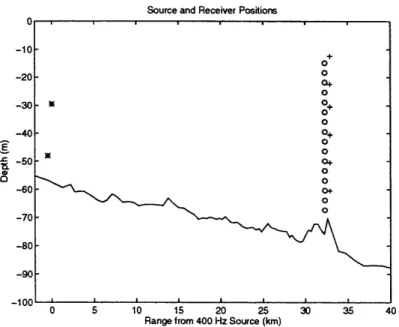
2-1 Source positions are noted by "*". The 400 Hz source is the shallower

of the two. WVLA hydrophone positions are noted by "o" and the

thermistors on the array are marked as "+". ... . 34

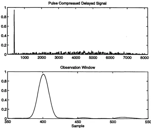
2-2 Circular convolution of an ideal delayed 400 Hz transmitted sequence with an ideal non-delayed transmitted sequence. Both sequences have been zero-padded from length 7129 to length 8192. The lower frame is

a window of the full output above. ... 38 2-3 Typical 400 Hz arrivals at the WVLA hydrophones. The sets of 16

3-1 _{Mode rejection levels from mode-filter outputs, A,(*), A2(x), A3(o),} and A4(+), as a function of array tilt. The four plots represent tilted

inputs of pure mode 1, mode 2, mode 3, and mode 4 arrivals. These plots use mode filters and mode arrivals generated from the same

typ-ical SWARM SSP. ... 46

3-2 Mode rejection levels from mode-filter outputs, A₁(*), A2(x), A3(o),

and A4(+), as a function of transmission number. The four plots are

based on a series of untilted inputs of pure mode 1, mode 2, mode 3, and mode 4 arrivals, where the mode filters and mode arrivals are generated from the same series of SSPs. . ... 48 3-3 Mode rejection levels from mode-filter outputs, A,(*), A2(x), A3(o),

and A4(+), as a function of transmission number. The four plots are

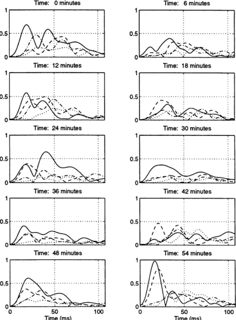
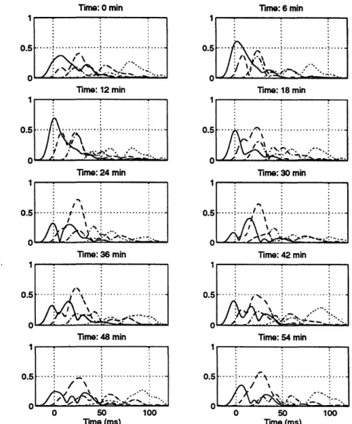
based on 1 degree tilted inputs of pure mode 1, mode 2, mode 3, and mode 4 arrivals, using mode filters and mode arrivals generated from the SSPs separated by 30 seconds. . ... . 50 3-4 Mode Coefficient outputs, Al(solid), A2(dashed), A3(dot-dash), and

A4(dotted), as a function of time. The ten plots depict the arrival

structure for the first of 22 captured sequences out of ten sequential transm issions . ... ... ... ... 52 3-5 Mode coefficient outputs, Ax(solid), A2(dashed), A3(dot-dash), and

A4(dotted), as a function of time. The ten plots depict the arrival

structure for every other sequence from the first to the 19th of 22 captured sequences from the time zero transmission in Figure 3-4. . . 54 3-6 Average correlation coefficients for outputs, A, (solid), A2(dashed), A3

(dot-dash), and A₄(dotted), as a function of elapsed time. The average is taken over the ten transmissions of Figure 3-4. . ... . 55

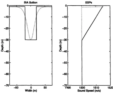
4-1 An illustration of the SIA approximation for solitons (left), and the idealized SSPs (right) used to model the interior and exterior regions of the SIA soliton. The dotted curve represents the exterior or back-ground region, and the solid curve represents the interior. ... 59 4-2 Propagation of four modes through 32 km of an idealized wave guide

with one 200 meter soliton at the 20 km point. The solid curves are the absolute value of coherent sums of the J2 = 16 dotted individually scattered arrivals. Starting amplitudes for mode 1 through 4 were 1.0,

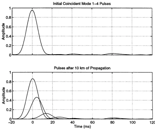
0.8, 0.6, and 0.4 respectively. ... .... . . 60 4-3 Propagation of four modes through 32 km of an idealized wave guide

with 200 meter solitons at the 10 and 20 km points. The solid curves are the coherent sums of the N2 x N2 = 256 dotted individually scattered arrivals. Initial mode 1 through 4 amplitudes were 1.0, 0.8, 0.6, and

0.4 respectively... 62

4-4 Simulated mode coefficient outputs, AI(solid), A2(dashed), A3

(dot-dash), and A4(dotted), for propagation through seven idealized

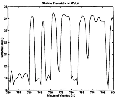
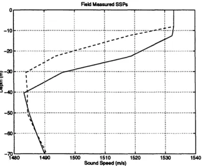
soli-tons. The solitons propagated toward the receiver in lock step at 0.8 m/s. The ten plots depict the arrival structures for sequential realiza-tions at six minute intervals ... 64 4-5 Time-series of temperature at a depth of 12.5 meters on the WVLA. . 65 4-6 Field measured SSPs for use in the pulse-propagation model. The

dashed line is representative of a standard SSP with no soliton. The solid line represents the soliton SSP. . ... 66 4-7 Mode shapes for field measured (SWARM) SSPs. The dashed lines are

the 355 Hz (thin lines) and 445 Hz (thick lines) mode shapes corre-sponding to the standard SSP with no soliton. The solid lines are the same modes for the soliton SSP. The dotted line at 68 m indicates the

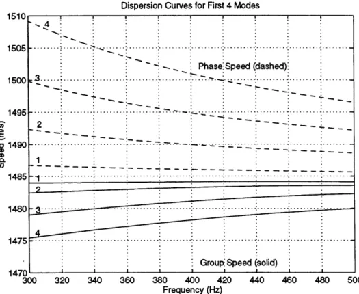
4-8 Phase and group speeds for the standard field measured SSP. Mode 1 has the lowest phase speed and the highest group speed. The remaining phase speeds increase monotonically with mode number, and the group speeds decrease monotonically with mode number... 69 4-9 Effects of mode and frequency dispersion on single mode transmissions

over 32 km. The transmissions include no soliton scattering or intrinsic mode attenuation. The attenuation in the higher modes is due solely to frequency dispersion. . ... ... 71 4-10 Effects of mode and frequency dispersion combined with intrinsic mode

attenuation on single mode transmissions over 10 km. The transmis-sions include no soliton scattering. . ... . 72 4-11 Mode coupling effects of the bottom topography shown in Figure 2-1

when the SSP is a modified version the "non-soliton" SSP of Figure 4-6. The "No Ducting" modification consists of imposing the 50.5 m temperature from 50.5 m to the bottom depth, and the "Ducting" modification consists of imposing the 60.5 m temperature from 50.5 m to the bottom depth. The thinner lines in this figure represent predicted arrival shapes for modes that propagate adiabatically. . . . 74 4-12 Comparison of fine scale coupled mode arrivals using 24 m (solid) and

48 m (dotted) step sizes. The 32 km wave guide under evaluation was generated from range propagated WVLA thermistor records. ... 78

5-1 The mean (-), median (...), standard deviation (-.), and interquartile

range (- -) of an unscattered mode 1 arrival plotted as a function of noise cutoff level. The median reaches its correct value of zero at a noise cutoff level of -38 dB relative to the peak of the arrival. ... 82

5-2 The solid line shows the mode number space history of one of the 620 subarrivals that would make up the mode 1 arrival from a six mode transmission through the 10 SIA soliton waveguide that is indicated by the dotted lines ... 83 5-3 Random realizations of test waveguides with from 10 to 35 200 m SIA

solitons over 32 km. The first soliton is placed randomly about 2.5 km from the source, and the remainder are added randomly from there, with an average of 450 m between leading edges. . ... 86 5-4 Single realizations of mode 1 (solid), mode 2 (dashed), mode 3

(dot-dash), and mode 4 (dotted) arrivals for 0 to 35 200 m SIA solitons over 32 km. The simulated waveguides used are similar to those shown in Figure 5-3. The simulated source depth is 27 m in 68 m of water, and the compressional wave attenuation in the bottom is .046 dB/m at 400 Hz. Note: Mode 4 arrivals are not visible at this level of attenuation. 87 5-5 The same scenario as Figure 5-4, except the compressional wave

atten-uation in the bottom has been reduced from .046 to 0.0115 dB/m. . . 88 5-6 Histograms for peak position of mode 1 arrivals for 5 through 40

ran-dom solitons. The solitons start about 2.5 km from the source with an average separation of 450 m between soliton leading edges. Time zero corresponds to the PAM1 arrival. . ... ... . . . . 89 5-7 The average mean (-), median (- -), and peak (- --) lag with respect to

the pseudo-adiabatic arrival, and standard deviation (-.) of scattered mode 1 arrivals plotted as a function of the number of solitons placed between the source and the receiver, where the solitons are added start-ing from the source end. The upper three lines are all bias measures, and the lower line is a measure of spread. ... . . . . . 90

5-8 The average mean (-), median (- -), and peak (- - -) lag with respect to

the pseudo-adiabatic arrival, and standard deviation (--) of scattered mode 1 arrivals plotted as a function of the number of solitons placed between the source and the receiver. The upper curves, averages over 50 realizations, represent the case where the solitons are added starting at the receiver end. The lower set of curves is replotted from figure 5-5. 60 solitons is essentially saturation, and the same points are used in both sets of curves. ... 91

5-9 Time dependent waveguide with two sets of six SIA solitons. The upper frame shows the starting positions, the middle frame shows the positions five hours later, and the lower frame is plot of peak position bias (re PAM1) as a function of time. The solitons propagate in lock-step, traversing 48 m per minute, the time between each peak position data point (o). The mean arrival data is also in one minute increments, but the points are connected by a solid line. . ... 96

5-10 Waterfall of mode 1 arrival patterns from the time dependent waveg-uide with two sets of six SIA solitons. The 300 peak positions in the lower frame of Figure 5-9 were picked from these arrival patterns. . . 97

5-11 Snapshots of the arrival shapes for all eight modes propagated in the Figure 5-10 simulation. The left hand column shows the minute 1 ar-rival shapes and the right column shows the minute 300 arar-rival shapes. The thicker lines are the scattered arrival shapes, and the thinner lines show the corresponding unscattered mode arrivals. The eighth mode is only minimally excited by the source at 27 m depth, and it undergoes the most attenuation, so it is not even visible as an unscattered arrival. 98

5-12 A comparison of mean (-) and peak (o) arrival time as function of the number of evenly spaced solitons in a 32 km waveguide. The first soliton is always 200 m from the source and the last soliton is roughly 32 km divided by the number of solitons away from the receiver. . . . 100 5-13 The top graph shows 12.5 m depth temperature readings from the 2

hrs of thermistor data used to simulate modal excitation levels. The middle graph shows the resulting modal excitation levels for mode 1 (solid), mode 2 (dashed), mode 3 (dot-dash), and mode 4 (dotted). Mode 5 is similar in magnitude and used as an input to the model, but it is omitted from this figure to avoid clutter. The lower graph shows the output bias levels corresponding to the excitation inputs shown in the middle graph. The solid line is the mode 1 arrival envelope peak arrival time in excess of the PAM1 arrival time and the dotted line is the mode 1 arrival envelope mean arrival time in excess of the PAM1 arrival tim e . . . . 101 5-14 Pycnocline displacements from an Orr backscatter record compared to

a thermistor string record using a propagation speed of .62 m/s over the distance between the back scatter instrument and the thermistor string at each backscatter reading ... ... 103 5-15 Distribution of peaks for the mode 1 arrivals of simulated transmissions

using sequential WVLA thermistor string generated waveguides. The sequential 32160 by 68 m waveguides are separated by six minutes. The size of each arrival dot is scaled by the amplitude of the peak arrival. The upper frame includes a plot of the PAM1 arrival time in conjunction with the individual peak arrival times; the zero reference on the arrival time axis corresponds to 21.6 seconds. The lower frame plots the bias or offset of the peak arrivals relative to the PAM1 arrival time for each realization ... 105

5-16 Distribution of peaks for the mode 2 arrivals corresponding to the mode 1 arrivals of Figure 5-15. The upper frame includes a plot of both the PAM1 arrival time (dotted line) and PAM2 arrival time (solid line), in conjunction with the individual peak arrival times; the zero reference on the arrival time axis corresponds to 21.6 seconds. The lower frame plots the bias or offset of the mode 2 peak arrivals relative to the PAM2 arrival time for each realization. . ... .. 106 5-17 30 minute bin averaged IQR measurements and the WVLA

tempera-ture profile for the simulation test period. The profiled temperatempera-tures range from 7.2 to 25.9 degrees C. The top frame is for mode 1 and the bottom is for mode2. ... 108 5-18 A comparison of 1 hour bin averaged IQR levels for the simulated

mode 2-4 data (solid lines) and a 1 hr bin average of the Standard Deviation of the Temperature at 22.5 m depth over the previous 4.3 hrs (dashed lines). The standard deviation of the temperature is in

tenths of a degree centigrade to facilitate comparison with the IQR levels in m illiseconds ... 110 5-19 Cross-correlations of 1.4 hr averaged peak height fluctuations for mode

1 (solid), 2 (dashed), 3 (dot-dashed), and 4 (dotted) with the corre-sponding 1.4 hr averaged mode 1 IQR (spread) levels. ... 111

6-1 Distribution of SWARM Mode 1 Peak arrival times. The zero refer-ence is at an arrival time of 21.985 seconds. The plotted transmissions occurred every six minutes, with each transmission producing 22 se-quence arrivals over a two minute period. The location of the highest peak in each sequence is plotted. Though not evident in most cases, there are gaps in the record that range from single lost transmissions to occasional larger gaps of up to two hours in duration. . ... . 116

6-2 Predicted current effects on PAM1 arrival time plotted with the dis-tribution of peak arrival times shown in Figure 6-1. The solid curve is based on the mean current between 39 and 59 m depth and the dotted curve is based on the average current between 11 and 67 m depth. .. 118 6-3 Predicted temperature fluctuation effects on PAM1 arrival time (solid

curve) plotted with the distribution of "current-corrected" peak arrival times. The solid curve is zero mean (by definition) and offset from the data for convenience ... 119 6-4 Mode 1 peak arrival time bias histograms for the data shown in Figure

6-1 and the model distribution shown Figure 5-15. The bias measure-ments are relative to estimated PAM1 arrival times (i.e. the leading edge) for the data and calculated PAM1 arrival times for the model. . 120 6-5 Mode 1 arrival spread, as measured by the IQR of the arrival

enve-lope (unscattered IQR is about 7.2 ms). The upper frame is plot of the spread when averaged over each transmission (22 sequences per transmission). The lower frame shows bin averaged spreads for five bin widths ranging from 1.4 to 4.1 hrs. . ... 122 6-6 Power Spectral Density of the bin averaged spreads shown in the lower

frame of Figure 6-5 ... ... 124 6-7 WVLA temperature as function of time and depth overlaid by the 1.4

hr bin averaged IQR of mode 1 arrivals at the WVLA. The tempera-tures in this figure range from 7.2 to 26.5 degrees C... . 125 6-8 A comparison of 1 hour bin averaged IQR levels for the SWARM

data (solid line), the corresponding propagated thermistor string model (dotted line), and the Standard Deviation of the Temperature at 22.5 m depth over the previous 4.3 hrs (dashed line). The standard deviation of the temperature is in tenths of a degree C to facilitate comparison with the IQR levels in milliseconds. . ... 127

6-9 A comparison of 1.4 hr averaged peak intensity fluctuations and the corresponding 1.4 hr averaged IQR levels for the SWARM data. The peak intensity fluctuations are plotted in terms of relative loss to pro-vide a signal that is in phase with the spread fluctuations. . ... 128 6-10 A comparison of 1.4 hr averaged peak-height fluctuations for the first

four modes of the SWARM data. Mode 1 is solid, mode 2 is dot-dashed, mode 3 is dashed, and mode 4 is dotted. . ... 130 6-11 Cross-correlations of 1.4 hr averaged peak height fluctuations for mode

1 (solid), 2 (dashed), 3 (dot-dashed), and 4 (dotted) with the corre-sponding 1.4 hr averaged mode 1 IQR (spread) levels for the SWARM data . . . . 132 6-12 Mode 1 (solid), mode 2 (dashed), mode 3 (dot-dashed), and Mode 4

(dotted) peak arrival time leading edge (connects earliest peak arrivals in 1.1 hr bins) and 1.4 hr bin average mean peak arrival times. The leading edges for modes 2-4 are bracketed between the two mode 1 solid lines, and the mean arrivals for modes 2-4 are positioned above the upper solid line... ... 134 6-13 Distribution of SWARM 224 Hz Mode 1 Peak arrival times. The zero

reference is at an arrival time of 22.453 seconds. The plotted transmis-sions occurred every five minutes. Only 8 sequences (every 4th from 1 to 29) are shown of the 29 available. An upshifted leading edge of the 400 Hz peak arrival distribution is also shown for comparison. The later zero reference time, relative to Figure 6-1, stems from the

difference in source mooring locations. . ... .... 135 6-14 Average arrival time difference between the 224 Hz PAM1, PAM2, and

PAM3 arrivals and the 400 Hz PAM1 arrival. The arrival times are based on 12 hour average SSPs at the WVLA employed in a range independent fashion over a distance of 32 km. . ... . 138

6-15 224 Hz 1.4 hr bin averaged peak arrival times and peak heights. Mode 1 is solid, mode 2 is dashed, and mode 3 is dotted... 139 6-16 Power spectral densities for the 224 Hz 1.4 hr bin averaged peak arrival

time and peak height time series of Figure 6-15. Mode 1 is solid, mode 2 is dashed, and mode 3 is dotted. . ... . 140 6-17 Comparison of 224 Hz and 400 Hz 1.4 hr bin averaged IQR (spread).

The IQR of an unscattered 224 Hz pulse would be about 37 ms (7 ms for a 400 Hz pulse) ... ... 141 A-1 Relative positions of transponder balls around the WHOI Vertical Line

Array (WVLA). Transponders were interrogated every four minutes by a pinger at the base of the array. Round trip travel-time to the top hydrophone of the array was recorded. . ... 150 A-2 A simple form drag model for deflection of the WVLA where the drag

force on the cable is all applied at the midpoint. The 20 cm/s current shown would create a displacement of about .5 m at the top hydrophone.151 A-3 The first (..) and fourteenth (-) depth bins of a 16 channel

bottom-mounted acoustic Doppler current meter (ADCP) moored about 3 km

from the WVLA. ... 154

A-4 Travel-time fluctuation data-vectors associated with the three transpon-der ball paths used to navigate the WVLA ... 155 A-5 Model vectors of an over-determined least-squares inversion of the

nav-igation data for north and east displacement of the hydrophone array. 156 A-6 Model vectors of a least-squares inversion of the navigation data for

north displacement, east displacement, and an average deviation in sound speed common to all three transponder return path integrals. . 159 A-7 A least-squares inversion for sound speed deviation produces

fluctua-tions similar those observed in a 12.5 meter depth thermistor record that has been converted to sound speed. . ... 160

A-8 A least-squares inversion for sound speed deviation produces fluctua-tions similar those observed in a 12.5 meter depth thermistor record that has been converted to sound speed. ... . . . . . 163

A-9 A least-squares inversion for sound speed deviations yields an 11.0/11.5 kHz path sound speed fluctuation (solid line) that is very similar those

observed in a 12.5 meter depth thermistor record (dashed line). . . . 164

A-10 12.0 kHz path travel-time fluctuations (upper line) are very similar those calculated by taking the range to the transponder and back di-vided the average of the WVLA soundspeeds at 40, 50, and 60 meters

depth ... 165

B-1 A comparison of single hydrophone pulse arrivals computed from the PPM (solid) and KFS (dotted) methods. The modeled waveguide uses the SWARM SSPs shown in Figure 4-6, with coupling from one SSP to the other occurring at 13,000 and 18,000 m. The source depth is 27 m and the receiver depth at all five ranges is 50m. ... . 169

B-2 An eight soliton waveguide (upper panel) and two corresponding ar-rivals computed from the PPM (solid) and KFS (dotted) methods. The modeled waveguide uses the SWARM SSPs shown in Figure 4-6 to simulate the solitons. The source (*) depth is 27 m and the receiver

(o) depth at both ranges is 50m ... 170

B-3 Single hydrophone RIP pulse arrivals computed from the PPM (solid) and KFS (dotted) methods using various source depths with the re-ceiver depth fixed at 50m. . ... ... 171

C-1 Effects of linear internal wave scattering on mode propagation. The results shown are the average of 50 trials using a sound-speed per-turbation model with a range and depth averaged < (Sc/co)2 > of 1.4 x 10-' . The mode shapes used in the coupling equations were from the standard field measured SSP at 400 Hz. . ... 179

C-2 Asymptotic behavior of SI + 1 for mode 1. The plotted quantity de-creases to the asymptotic value of the growth rate factor X. The mode shapes and attenuation parameters used in the coupling equations were from the standard field measured SSP at 400 Hz. . ... . . 181

C-3 Mean sound speed profiles obtained from the WVLA thermistor records. The solid line is an average over yearday 211-217, and the dashed line is averaged over yearday 211 only. The dotted SSP is taken from early in yearday 211 when no solitons were at the WVLA. All three are extrapolated for depths above 12.5 m and below 60.5 m. . ... 183

C-4 Magnitudes of discrete coupling matrix coefficients using a 48 m step size with three different background profiles. The solid lines are com-puted using the yearday 211-217 mean profile, the dashed lines are from the yearday 211 mean profile, and the dotted lines are computed

using the yearday 211 "no soliton" SSP. ... 184

C-5 Predictions of mode 1 arrivals made with three different background profiles. The solid lines are computed using the yearday 211-217 mean profile, the dashed lines are from the yearday 211 mean profile, and the dotted lines are computed using the yearday 211 "no soliton" SSP. 185

C-6 Twelve hours of predicted mode 1 arrivals using the yearday 211 mean profile and the yearday 211-217 mean profile. . ... . . 186

D-1 A comparison of reciprocal transmissions through an asymmetric SIA soliton waveguide (upper frame). Mode 1 through 4 arrivals as well the time domain pulse at a single transducer (27 m) are shown for both the forward and reciprocal transmissions. The source/receiver depth is 27 m for both transducers ... 190 D-2 A comparison of reciprocal transmissions through a strong front (upper

frame). Mode 1 through 4 arrivals as well the time domain pulse at the receiver are shown for both the forward and reciprocal transmissions. The source/receiver depth is 50 m at 0 km and 27 m at 32 km... . 191

List of Tables

2.1 Data set outline for the WVLA. Tapes 1 through 8 contain telemetered data that is sometimes broken up when the ship was out of range. Tapes 9 and 10 contain internally recorded data that fills in most of the gaps in the telemetered data. ... 35

4.1 Intrinsic mode attenuation parameters, -, for various mode numbers. Values for both a soliton SSP and the standard field measured SSP

without a soliton present are given. ... 71

5.1 Subarrival statistics for the simple two mode 50/50 scattering scenario where there are four equally spaced increments and the difference be-tween the PAM1 and PAM2 arrival times is AT = 1. ... 94 5.2 Zero-lag cross correlations between 1.4 hour bin averaged mode 1-4

peak heights and mode 1-4 mean spread levels. ... 112

6.1 Zero-lag cross correlations of 1.4 hour bin averaged peak heights for the SWARM data and the simulated data of Chapter 5. The unmixed data (modes 1 and 2) are shown in Figures 5-14 and 5-15; the cross-talk contaminated is from the same source, with incoherent mixing based on the "Average" filter performance matrix shown in section 3.3.2. . . 131

6.2 _{Zero-lag cross correlations between 1.4 hour bin averaged mode 1-4} peak heights and mode 1-4 mean spread levels. The spread measure-ment employed for these cross-correlations is the standard deviation of peak arrival times over a transmission. . ... 132 6.3 Hypothetical range independent travel times corresponding to daily

averaged SSPs at the WVLA. The travel time differences between 224 Hz and 400 Hz modes are also listed. . ... 136

Chapter 1

Background

The Shallow Water Acoustics in a Random Medium (SWARM) experiment [1], con-ducted off the coast of New Jersey near the continental shelfbreak in July and August of 1995, was dedicated to furthering our understanding of acoustic mode scattering effects of both linear internal waves and nonlinear solitary internal waves (solitons) in shallow water.

1.1

Solitons

A stratified ocean will support a variety of internal waves, the most common being the internal equivalent of a linear surface gravity wave. In the deep ocean, these waves are generally isotropic in direction and have frequency/vertical mode power spectra that are red and dominated by the first few modes. The canonical Garrett-Munk (GM) spectrum [3] normally provides a good model for the observed power spectra in deep water. The story is quite different along the United States East Coast continental shelf and other shallow regions, where the linear waves are non-isotropic and the internal wave field can also be heavily influenced by nonlinear solitary waves.

Internal solitons appear to be generated in groups or packets at the continental shelfbreak when the tide shifts from an ebb to a flood. Each "developed" packet

usu-ally contains six to twelve solitons that are large enough to have a surface expression on radar, so the term "solitary wave" is something of a misnomer in this case. An account of the first observation of a surface solitary wave, made by John Scott Russell in 1834, is provided by Strang [4]:

I was observing the motion of a boat which was rapidly drawn along a narrow channel by a pair of horses, when the boat suddenly stopped... not so the mass of water in the channel which it had put in motion; it accu-mulated round the prow of the vessel in a state of violent agitation, then suddenly leaving it behind, rolled forward with great velocity, assuming the form of a large solitary elevation, a rounded, smooth and well-defined heap of water, which continued its course along the channel apparently without change of form or diminution of speed. I followed it on horseback, and overtook it still rolling at a rate of some eight to ten miles an hour, preserving its original figure some thirty feet long and a foot to a foot and a half in height. Its height gradually diminished, and after a chase of one or two miles I lost it in the windings of the channel.

This surface soliton can be modeled by the Korteweg-de Vries (KdV) equation,

77t

where the wave solution,

(- t) = sech2 (\z - ct)) (1.2)

has a single hump whose height, ac, is proportional to the speed at which it travels to the right [4].

In contrast to the surface soliton's hump, internal solitons normally appear as a sech2 shaped depression in the pycnocline. In covering some theoretical aspects of internal solitons, Apel et al. [5] provide a solution for the following internal wave

KdV equation,

77t + cr7, + a0p7x + 07l== = 0, (1.3) namely,

n(x, t) = 7osech2 (X Vt), (1.4)

where the soliton phase speed, V, is,

V = c + a70/3 (1.5)

and the characteristic width, A, is given by, 123

A2 1 (1.6)

a77o

For a simple two-layer ocean density model, the constants are C= g(p2-pj)hjh 2

i

(1.7)

Where h, and h2 are the thicknesses of the upper and lower layers, and p, and p2 are

the respective densities. From the characteristic width formulation, we see. that 77o will have the same sign as a, so for the most common case of a shallow pycnocline over a deeper layer (i.e. p2h2 < p1 h), ,7 will be negative (i.e. downgoing). Employing this

model with reasonable 2-layer approximations for a large SWARM soliton, qo = 20 m, h, = 15 m, h2 = 55 m, and gAp/p = .01 m/s2, we predict a rather typical soliton

phase speed of V = .8 m/s and the wave shape shown in Figure 1-1. The linear phase speed, c, for this case is 0.34 m/s for comparison.

The internal solitary wave packets are often so numerous and closely spaced on the New Jersey shelf in summer that a nearly continuous train of solitons can pass a fixed instrument over the course of several hours. This is illustrated in Figure 1-2, where an

Intemal Soliton

-150 -100 -50 0 50 100 150

Width (m)

Figure 1-1: A simple two-layer model of an internal soliton, with the upper layer,

hi = 15 m, lower layer, h2 = 55 m, and reduced gravity, gAp/p = .01 m/s2. The 20

m depression propagates at a phase speed, V = .8 m/s.

array of thermistors attached to the WHOI Vertical Line Array (WVLA) records the passage of several packets over a six hour period. The mixture of time and space in this figure creates a distorted view of the soliton shapes, but this can be approximately corrected by applying a constant phase speed to a selected soliton, thus transforming the time coordinate into a space coordinate. This has been accomplished in Figure 1-3, where the time series for the prominent soliton in the lower frame of Figure 1-2 has been transformed into a properly scaled space representation.

1.2

Acoustic Impact of Solitons

The first investigation of the acoustic impact of solitons was reported by Zhou et al. [6] in 1991. This paper generated interest in the subject, and further strides have been made in the several investigations that have followed [1, 2, 7, 8, 9].

1.2.1

Time Spreading

Internal solitons often have first mode displacements at the pycnocline ranging from 10 to 20 meters. These large displacements occur over relatively short wavelengths (Figure 1-3), creating strong horizontal gradients in soundspeed, which thus produces coupling between acoustic normal modes. Differences in the acoustic modal group velocities cause time spreading of pulses as energy is transferred between different

U

I

I

I

I

20

60

Sditans Passin WVLA m 31 Juiv 1995

)Z

-4 0

Figure 1-2: Time and space interpolation of four thermistor records. The thermistors were attached to the WVLA at water depths of 12.5, 20.5, 30.5, and 40.5 meters and sampled at 30 second intervals.

Soliton Dimensions (m) x -20 0) -60 0 50 100 150 200 250 300 350 Length

Figure 1-3: Space transformation of the time series for the prominent soliton in the lower frame of Figure 1-2. All six available thermistors are used, so the depth spans 12.5 to 60.5 meters. The dimensions shown are properly scaled for soliton with a combined phase and advection speed of .8 m/s.

modes. In the SWARM waveguide, mode 1 has the highest group speed, so the energy that transits in other modes for a portion of the trip is delayed with respect to energy that traveled exclusively in mode 1. This causes the spread of mode 1 energy to be all in one direction (i.e. there is a positive bias in the mean and median travel-time of mode 1 energy relative to an unscattered mode 1 arrival travel-time). Higher modes may have some energy coming in earlier (from traveling partially in lower modes) and some coming in later (from traveling partially in higher modes), so there may be negative, positive, or even zero bias in travel-time for these modes. As shown by Colosi and Flatti [10] the coupling caused by linear internal waves is similar, but reversed, in deep water where mode 1 generally has the lowest group speed.

Repeated coupling processes create mode arrivals that are sums of numerous "mode multipaths" that propagate through the range and wavenumber (mode num-ber) space between the source and the receiver. Constructive and destructive interfer-ence between "mode multipaths" creates peaks and nulls in the arrival pattern. The detailed interference patterns are very sensitive to the spacing between the coupling events. Thus, given the tidal period variations in the size and numbers of solitons between the source and receiver and the continuous variations in soliton position and spacing (caused by their differing phase speeds), significant temporal variations in arrival-time patterns are to be expected.

1.2.2

Attenuation

Another effect of the coupling of mode 1 into higher modes is the apparent increased attenuation of mode 1 discussed by Zhou et al. [6]. In general modal attenuation is greater for higher mode numbers, so coupling is an energy sink for low modes and a source for higher modes. This mode-stripping along with long-term variations in the amount of coupling and short-term variations in interference patterns creates significant variability in the apparent attenuation of mode 1 energy.

1.3

Outline of Thesis

Chapter 2 discusses SWARM data that are relevant to this thesis, along with other details such as experiment geometry, signal characteristics, data storage requirements, and pulse-compression schemes. Several issues associated with mode-filtering are then addressed in Chapter 3: a basic theory of normal mode propagation; analysis of possible errors in the mode filters used; and the accuracy of the filter outputs relative to the actual mode arrivals.

A model for the propagation of normal modes through a 2-D waveguide with solitons is developed in Chapter 4. Chapter 5 discusses pulse propagation simulations using two different forms of the model. The simplest form of the model, which uses Preisig and Duda's [2] sharp interface approximation (an inverted square-wave) for solitons, was tested by varying the numbers and locations of solitons and the amount of bottom attenuation. In observing the sensitivity of mode arrival statistics to changes in the model parameters, candidate statistics for quantifying the spread and bias of mode arrivals were evaluated. The second, more complicated, form of the model is based on range propagated thermistor string records, so it models the effects of both linear and nonlinear internal waves. It is used to try to model the temporal variations in the SWARM waveguide during the time of the actual experiment.

Chapter 6 discusses the analysis of mode 1-4 arrivals for the 400 Hz source and the mode 1-3 arrivals for the 224 Hz source. The narrow pulse width of the 400 Hz source provided much better data, and it receives a greater share of our attention. Chapter 7 lists the conclusions reached and proposes outlines of future investigation.

Chapter 2

Data Collection

2.1

Experiment Geometry

The sixteen element WVLA, moored in 70.5 meters of water off the New Jersey coast, operated continuously for seven days. Tomography sources with carrier frequencies of 224 and 400 Hz were moored about 32 km shoreward on a compass heading of 3000 and transmitted to the WVLA. The resulting acoustic path was anti-parallel to the primary propagation direction for shelf generated internal waves. The temperature profile in the vicinity of the WVLA was monitored by six thermistors attached to the array at various depths. Figure 2-1 illustrates the 2-D geometry of the experiment.

2.2

Source Signals

The 400 Hz (100 Hz bandwidth) tomography source produced a 511 digit, phase-modulated signal sequence with a digit length of 4 cycles, for a total of 5.11 seconds per sequence. The sequence was repeated 23 times during each transmission, for a transmission time of 117.53 seconds. The 400 Hz transmissions started on the hour and were repeated every six minutes. They were received at the WVLA about 22 seconds later.

-10 -20 -30 -40 . -50 -60 -70 -80 -90 -inn

Source and Receiver Positions

0 5 10 15 20 25 30 35 40

Range from 400 Hz Source (kin)

Figure 2-1: Source positions are noted by "*". The 400 Hz source is the shallower of the two. WVLA hydrophone positions are noted by "o" and the thermistors on the array are marked as "+".

The 224 Hz (16 Hz bandwidth) tomography source produced a 63 digit sequence, phase-modulated signal with a digit length of 14 cycles, for a total of 3.9375 seconds per sequence. The sequence was repeated 30 times during each transmission, for a transmission time of 118.125 seconds. The transmissions were repeated every five minutes, starting on the hour, five after, etc. They were received at the WVLA about 22.5 seconds later.

2.3

Receiving Array

The WVLA had hydrophones spanning water depths from 14.9 to 67.4 m. The hydrophones could not be placed any higher in the water column without experiencing surface wave effects. The sixteen hydrophones were sampled at 1395.089286 Hz six of the seven days the array was deployed. The sample rate for the remaining period was 1953.1250 Hz. The data were normally telemetered back to a moored research vessel (R/V Oceanus) stationed several kilometers away, but a limited amount of internal

+ 0 0 0+ 0 0₊ 0 O o+ 0 -0 II _-O si0 0 n

Table 2.1: Data set outline for the WVLA. Tapes 1 through 8 contain telemetered data that is sometimes broken up when the ship was out of range. Tapes 9 and 10 contain internally recorded data that fills in most of the gaps in the telemetered data.

storage was available and automatically utilized when the ship was out of range. The non-integer sample rates were dictated by the system's analog to digital converter. The equipment provided a very accurate sample rate, but the sample frequencies were limited to

5MHz

Sample Rate = n (2.1)

256 * ni * 2n2

In our case, nl = 7 or 5, and n2 = 1.

The data were stored on tapes, with about 27 files per tape. Each file contains up to 160 records which are approximately 1 megabyte each. The records consist of 32768 two byte digitized voltage samples for each of the sixteen hydrophones. The sample rate of 1395.089286 Hz, yields about 23 seconds of data per record and 62 minutes of data per file. Seven days of data required over 25 gigabytes of storage,

and an outline of the entire data set is given in Table 2-1.

The combination of the 1395 Hz sample rate and sequence length for the 400 Hz source yields 7128.9063 samples per sequence, and the 224 Hz arrivals require 5493.1641 samples per sequence. Both of these numbers are rather cumbersome to

Tape Number First Last

Number of Files File File

1 16 210-19:54 211-10:48 2 7 211-16:43 211-22:58 3 2 212-01:09 212-01:11 4 1 212-01:50 212-01:50 5 14 212-03:27 212-17:01 6 32 213-02:02 215-06:01 7 29 215-06:27 216-11:41 8 18 216-13:04 217-06:49 9 34 210-19:50 214-05:13 10 30 214-00:34 217-17:50

deal with. An ideal combination of sequence length and sample rate would produce a radix-2 integer number of samples per sequence. During the period from about 1600Z day 213 to 1600Z on day 214, the sample rate was shifted from 1395 to 1953 Hz, and the resulting files only cover 44 minutes. Seven transmissions are removed from each 160 Mb file during this period.

There are two further data considerations. First is the location of the header on each file. The telemetered data files have headers at the beginning of the files. The internally recorded data have their headers are at the end. Second, as a consequence of the shifts between telemetered and internally recorded data, some files with less than 160 Mb were created during both the 1395 and 1953 Hz sampling periods. These files obviously contain fewer transmissions.

2.4

Signal Isolation

2.4.1

Sequence Capture

The 400 Hz arrivals at the WVLA can be analyzed one sequence at a time, but of the 23 sequences in a transmission, only 22 full sequences can be captured for analysis. The loss of one sequence is required to compensate for the uncertainty in the actual arrival time of the beginning of the first sequence in a transmission. The transmitted sequences have an ideal circular autocorrelation property that is unaffected by the starting point in a captured sequence.

In our case, sequence capture is accomplished by starting the first capture at a fixed time (26.85 secs) after the beginning the transmission. The fixed time for the first sample was chosen through a series of trials to be about 400 samples (depending on the particular transmission) or 280 msec prior to the start of the arrival of the second sequence. The earlier parts of the first sequence are discarded, and the last 400 samples are clipped from the second sequence to provide the data buffer for the beginning of the third sequence. This process continues through the sequences until

the last 400 samples of the 23rd sequence are clipped and discarded. The 22 sequences obtained in this manner are rounded to 7129 samples long, and have basically been circularly shifted to the right (i.e. delayed) by about 400 samples with respect to the transmitted sequence. In a similar manner, 29 sequences of the 30 transmitted can be captured from each 224 Hz transmission. The 224 Hz sequences are rounded to 5493 samples for analysis.

Changes in travel-time are estimated by capturing sequences using a fixed time delay after transmission and detecting the resulting circular shifts in the captured sequences. There are a non-integer number of samples between transmissions, so choosing the first sample to capture in a sequence creates an error between the desired fractional sample number and the allowable integer sample numbers. A correction for the time and phase error introduced by the sample error can be made by multiplying the base-band signal in the frequency domain by ei2₁r_(f+fc)a t_{, where f is the base-band}

frequency, fc is the carrier frequency, and At is the sample error divided by the sample rate. This correction step is accomplished in conjunction with pulse-compression.

2.4.2

Pulse Compression

The captured 400 Hz sequences are demodulated to baseband and then low-pass filtered by windowing in the frequency domain with a 90 Hz pass-band Blackman window. Pulse compression is also accomplished in the frequency domain through multiplication with the conjugate spectrum of the transmitted sequence. This is equivalent to a matched-filter circular convolution in the time domain [11].

If sequence lengths of 5493 and 7129 are maintained, mixed-radix DFTs must be used in the transforms between the time and frequency domains. These mixed-radix DFTs are too slow for practical application, so the data was zero-padded to a length of 8192 in order to employ a radix-2 FFT.

The circular convolutions of delayed and zero-padded signals with zero-padded transmitted sequences are not ideal. The resulting sidelobes (Figure 2-2) stem from

Pulse Compressed Delayed Signal

1000 2000 3000 4000 5000 6000

Observation Window

7000 8000

Sample

Figure 2-2: Circular convolution of an ideal delayed 400 Hz transmitted sequence with an ideal non-delayed transmitted sequence. Both sequences have been zero-padded from length 7129 to length 8192. The lower frame is a window of the full output above.

offsets in the location of the zeros. The sidelobe effects were eliminated from all analyses presented through SNR discrimination.

It is not necessary to save the entire output of the pulse compressed data. The relevant portions of the data are limited to an area around the peak arrival that encompasses the spread of energy caused by mode dispersion and coupling. A 200 sample ( 143 msec) observation window like that shown in Figure 2-2 is sufficient to capture the spread expected from modal dispersion over 32 km, but an additional 70 msec is required to accommodate the wander. Figure 3-3 shows some typical saved outputs of 400 Hz pulse-compressed arrival patterns for the hydrophones at the WVLA. Due to its wider pulse width, 358 msec are saved for the 224 Hz arrivals.

I I I I I I

· ·- . ... .. -- -- .. -- .- .--- .. ... I·-- -- I- U I . ...--

Time: 0 minutes -10 -20

E-30

Figure 2-3: Typical 400 Hz arrivals at the WVLA hydrophones. The are separated by 6 minutes.

sets of 16 arrivals

E

--

Chapter 3

Mode Filtering

3.1

Normal Modes

The two most frequently used representations of sound propagation in ocean acoustic waveguides are rays and normal-modes. Ray theory is perhaps more intuitive, but it is a high frequency approximation that is better suited to situations where the

acoustic wavelength is small compared to the dimensions of the sound channel. Our low frequencies and shallow waveguide are better suited to a modal analysis than ray theory.

The modal analysis of 400 Hz acoustic arrivals at the WVLA begins by treating the acoustic signal at each hydrophone as a sum of vertical modes

N

ph(t) = _ A,(t)O,(zh), (3.1)

n=1

where ,,(z) is the mode shape, A,(t) is the mode coefficient, and zh is the depth of the hydrophone in question. The number of propagating normal modes, N, as well as the mode shapes themselves are frequency dependent. The mode shapes are analogous to the eigenmodes of a vibrating string, and are formed by a constructive vertical interference pattern caused by a pair of up and down going plane-waves with the

same horizontal wave number. The highest possible normal mode number is roughly equivalent to the sound channel depth divided by the acoustic wavelength, where the up and down going pair of plane-waves would be propagating with a horizontal wave number approaching zero.

The six thermistors on the WVLA, which are sampled every 30 seconds, provided the soundspeed profiles needed for computing a time-dependent set of mode shapes using the KRAKEN [12] normal-mode code. The basis for this code, a numerical normal-mode solution of the Helmholtz equation at frequency w,

[V + k2(x, y, z, w)] p(z,y,z,w) = 0, (3.2)

where p(r, w) is the Fourier component of the pressure field, can be found in Jensen

et al. [13].

The KRAKEN [12] mode shapes are orthonormal in the sense that,

I

_P(Z)

so given p(z, t), A,(t) can be readily computed by applying the operator

(- Z) dz. _(3.4)

P(Z)

Since the pressure field, p(z, t), is only sampled at the sixteen hydrophone locations, the integral computation of the mode coefficients, A,(t), must be approximated by

A1(t)! p(zht)( (3.5)

h=1 P(Zh)

where Az is the spacing between hydrophones. This discrete sum can be easily im-plemented through matrix multiplication of mode shape vectors with 16 channel hy-drophone data vectors. This process of converting the 16 channels of hyhy-drophone data into N normal mode arrivals is referred to as narrowband direct-projection (NBDP)

mode-filtering.

An alternative, broadband direct-projection (BBDP) mode-filtering operates in the frequency domain, approximating the Fourier components of the mode arrivals as

16 P(Zh,f1j)On(Zh,fj)AZ

A.

(f)

?

1

(3.6)

h=1 p(zh)

where

p(zh,fj) = p(zh, t,)e-i2_{"(f)t"At. (3.7)}

The time domain mode coefficients can then be recovered through

A,(tm)

=

Z

A,(fn)ei

_(f)tmAf.

_(3.8)

The benefits of this method over NBDP depend upon the frequency dependence of the mode shapes over the bandwidth of the arriving signal. The cost of BBDP is in computation time; over 4000 different sets of narrowband mode filters are required for each frequency to cover the time-dependence seen in six days of data, so in the ideal extreme of a different set of ~n(fj)s for each of the 1000 frequency bins that cover the bandwidth of the signal, 4 million sets of mode filters would be have to be computed! The extreme case is not feasible, but there are compromises that can be explored.

Either DP method should work very well for the low modes that are adequately sampled by the WVLA. A typical SWARM mode 1 shape will yield,

6 01(zh)1(zh)Az = 0.9989, (3.9)

h=1 p(zh)

very close to the ideal output of 1.0. Higher modes have more energy outside the depths sampled by the WVLA, so the above "auto-filtration" degrades, yielding out-puts of 0.9949, 0.9881, 0.9803, 0.9681, 0.9269, and 0.8243 for modes 2 through 7, respectively. The higher modes suffer more from partial coverage than they do from

undersampling, so a simple output gain factor (like dividing the filter output by its auto-filtration level) may be useful if level comparisons between mode arrivals are to be made. However, an output gain factor will not provide relief from modal-crosstalk, which is also inherent with undersampling and partial coverage.

One must keep in mind that mode coefficient outputs of the mode-filtration are dependent on the quality of both the computed mode shapes and the measured pres-sure field. The most significant error associated with prespres-sure field meapres-surements is uncompensated array tilt. Deviations from a perfectly vertical array will cause phase

differences between hydrophones that degrade the mode coefficient computations.

3.2

Array Tilt

The designed navigation system for the WVLA was extensive and complete, with three transponder travel-times recorded at four hydrophones on the array. Unfor-tunately, the travel-times from one of the transponders to three of the hydrophones did not record properly, leaving just one channel (the shallowest hydrophone) fully navigated. Moreover, all of the navigation travel-times appear to be heavily influ-enced by small-scale temperature fluctuations caused by internal waves. The waves caused navigation travel-time changes that were three to five times larger than those expected from mooring motion. The time scale of these travel-time changes is on the order of the navigation sample rate (once every four minutes), consistent with soliton passage. The longer time-scale navigation travel-time changes are similarly out of proportion with expected motions of the array. They are probably due to path de-pendent temperature fluctuations, as well; thus these navigation data are considered largely unusable.

We can try to estimate the array tilt by hydrodynamics. The length of the of the mooring is approximately 60 meters and it has net buoyancy of 3230 Newtons.

a barotropic current will cause upper hydrophone displacements that are roughly proportional to the square of the current speed, giving 1 meter at 30 cm/s; 2 meters at 40 cm/s; and 3 meters at 50 cm/s. The current records obtained from a bottom-mounted acoustic Doppler current meter (ADCP), moored about 3 km from the WVLA, showed barotropic currents that seldom exceeded 30 cm/s, with occasional baroclinic currents from large solitons of up to 50 cm/s.

The effects of baroclinic currents on mooring motion are hard to predict, but the movement at the top hydrophone is certainly less than what would be produced by a barotropic current of the same magnitude. This line of reasoning predicts mooring motions that are generally less than a meter in amplitude at the top hydrophone (equivalent to 1 degree of tilt) with occasional excursions that might approach 2 me-ters. A more detailed analysis of the WVLA navigation data is provided in Appendix A.

3.3

Mode Filtering

3.3.1

Errors from Array Tilt

As mentioned earlier, phase differences caused by array tilt will cause errors when the 16 channels of acoustic data from the WVLA are converted to normal mode arrivals through mode-filtering. Figure 3-1 illustrates the effects of array tilt on some typical 400 Hz mode-filter outputs; the inputs are pure mode shapes from the same sound speed profile (SSP) as the mode-filter. With no tilt, all four mode filters do an exceptional job of passing their respective mode and rejecting all others. The mode-filters continue to perform acceptably for small deflections (less than 1 meter) of the upper hydrophone, but most become significantly degraded for deflections approaching 2 meters. With the exception of mode 2 rejection, the mode 1 filter performs robustly all the way to 2 meters of tilt.