An analysis of international transportation network

(1)

An Analysis of International Transportation Network

By Yu-Yen Chiu

Bachelor of Business Administration National Taiwan University, 2001

Submitted to the Engineering Systems Division in Partial Fulfillment of the Requirements for the Degree of

Master of Engineering in Logistics at the

Massachusetts Institute of Technology June 2005

MASSACHUSETTS INSTI E OF TECHNOLOGY

JUL

152005

LIBRARIES

The author hereby grants to MIT permission to reproduce and to

distribute publicly paper and electronic copies of this thesis document in whole or in part.

Signature of A uthor ... K ... .. ...

Eigineering Systems Division 7(4y 6, 2005

C ertified b y ... ...

V aplice

Executive Director-Master of Engineerl g inogistics Program hesis Supervisor

A ccep ted b y ... ... Yossi Sheffi Professor of Civii a tal Engineering Professor o#Engineering Systems Director, MIT Center for Transportation and Logistics

(2)

An Analysis of International Transportation Network

By

Yu-Yen Chiu

Submitted to the Engineering Systems Division on 6 May 2005 in Partial Fulfillment of the Requirements for the Degree of Master of Engineering in

Logistics

Abstract

This thesis discusses a network design problem based on a case study with a footwear company, which intends to minimize total supply chain costs by establishing a distribution network which bypasses its primary distribution center (DC). Through the new network, called the DC bypass network, the company ships products directly from its Asian factories to a logistics hub at an entry port in the US and then on to customers, a particular group of chosen customers.

We assess the project by comparing costs derived from a baseline and optimization model. A baseline model represents the company's existing logistics network while optimization models capture future supply chains with different scenarios. The models convert a real supply chain network into the relationships between nodes and links. Nodes indicate facilities while links refer to the flow of the product.

In brief, this case study is about how a company evaluates its transportation network. Methods to determine a specific location or multiple locations for the DC bypass operations are discussed. Furthermore, the robustness of an optimal solution will be measured through a sensitivity analysis. Other benefits include the reduction of lead time is discussed in the further research.

Thesis Supervisor: Christopher Caplice

(3)

Acknowledgements

First, I would like to thank Dr. Chris Caplice for his help on this project. He is a great thesis advisor, who always guides an efficient direction, brings in great ideas, and save me from the black hole of the thesis process.

Then, I would like to thank to my mother, Chunglien, for her unlimited, unconditional love and support. She believes that I can achieve everything, and thus so do I.

Finally, I would like to quote an old saying in Taiwan to express my gratitude to my classmates and friends I don't mention here, "There are too many people to thank to. Therefore, I would like to thank God for bringing these people to me."

(4)

Table 1-1 Table 3-1 Table 3-2 Table 3-3 Table 3-4 Table 3-5 Table 3-6 Table 3-7 Table 3-8 Table 3-9 Table 3-10 Table 3-11 Table 3-12 Table 3-13 Table 3-14 Table 3-15 Table 3-16 Table 3-17 Table 3-18 Table 3-19 Table 4-1 Table 4-2 Table 4-3 Table 4-4 Table 4-5 Table 4-6 Table 5-1 Table 5-2 Table 5-3 Table 5-4 Table 5-5 Table 5-6 Table 5-7 Table 5-8

List of Tables

Percentage of the Products Produced in Asia ... 12

Data Collection List ... 24

Average Pairs of Shoes per FEU Container ... 26

Door-to-Door All-W ater Ocean Freight... 27

Average Share of Ocean Freight... 27

Cost Breakdow n... 28

Adjusted Cost Breakdow n ... 28

Adjusted Cost Breakdow n According to a Particular Ratio ... 29

Lead Tim e (day) at Replenishm ent Link... 31

Unit Transportation Rate at Inland Transportation Link... 31

Unit Transportation Rate at Inland Transportation and Outbound Link... 32

Lead Tim e (day) at the DC Transfer Link... 32

Lead Tim e (day) at DC Transfer and Outbound Link ... 32

Historic Export Volum e at a Departure Port... 33

Handling Cost at a Departure Port ... 33

Historic Im port Volum e at an Arrival Port... 34

Handling Cost for the DC Bypass Operation... 35

Top 13 Custom ers ... 37

Tier-One Custom ers in the DC Bypass project ... 38

Top 10 Cities ... 38

Cost in Baseline M odel... 40

Group of Scenarios... 43

Notation of the Netw ork M odel... 44

Assum ptions of Initial Runs ... 44

Assum ptions of Forced Runs ... 44

Notation of the Formulation ... 46

Assum ptions of Selected M odels ... 52

Costs of Selected M odels... 52

Transportation Costs of Selected M odels ... 53

Notation of the Optim ized Netw ork M odel... 54

Tier-One Custom ers' Netw ork ... 55

Dem and of Tier-One Custom ers ... 56

Handling Costs of Selected M odels ... 58

(6)

List of Figures

Figure 1-1 Exam ple of a Logistics Netw ork... 8

Figure 1-2 Percentage of Sales ... 10

Figure 1-3 Location of the Products Produced in Asia... 11

Figure 1-4 Existing Footw ear Supply Chain... 13

Figure 1-5 Potential Footwear Supply Chain ... 15

Figure 3-1 Links in Shoe Co.'s Supply Chain... 30

Figure 5-1 Aggregation of the Tier-One Customer Demand ... 57

Figure 5-2 DC Handling costs which makes the DC bypass network undesirable ... 59

Figure 5-3 Bypass DC handling costs which makes the DC bypass network undesirable ... 60

Figure 5-4 Relationship between Facility Cost and No. of Facility for the DC Bypass Operation ... 61

(7)

1

Introduction

This thesis is mainly related to a network design problem based on a case study with a footwear company, hereafter called the "Shoe Co." The company intends to minimize total supply chain costs' by establishing a distribution network which bypasses its primary distribution center in Stoughton, hereafter called the "Stoughton DC." Through the new network, called the

distribution center bypass network, Shoe Co. proposes to ship product directly from its Asian factories to a logistics hub at an entry port in the US and then on to selected customers, hereafter called Tier-One Customers.

In this chapter, we will define a transportation network, introduce the background of Shoe Co. and its current operation, and identify the scope of the DC bypass project.

1.1 Fundamentals of a Transportation Network

Networks are widely used in our daily lives. They can be communication, electrical, logistics, or others. In this thesis, we focus on Shoe Co.'s transportation network, also called a distribution,

logistics, or supply chain network. A transportation network consists of facilities and links. Facilities can be factories, ports, distribution centers, retailer stores, or any place where raw

materials, work-in-process products, or finished products are manufactured, stored, or modified by value-added operations. Links are connections between facilities. They represent the

(8)

provides the structure for supply chain operations such as receiving, putting away, storage, picking, and the transport of products.

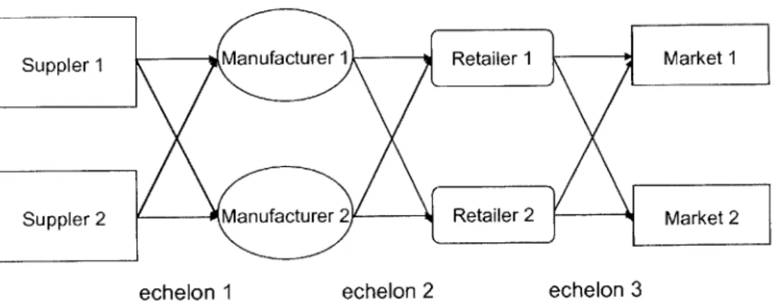
Figure 1-1 displays a simple supply chain network for a company. It is a three-echelon network that includes suppliers, manufacturers, retailers, and markets. Suppliers serve

manufacturers, which serve retailers, thus meeting the demand of two markets. Each echelon has two parties. Thus, there are 12 links between facilities in total.

Figure 1-1 Example of a Logistics Network

Suppler 1 Manufacturer 1 Retailer 1 Market 1

Suppler 2 Manufacturer 2 Retailer 2 Market 2

echelon 1 echelon 2 echelon 3

In real life, a supply chain network is more complicated because it involves more parties. A company's logistics network can involve many partners including suppliers, manufacturers,

distributors, retailers, carriers, third party service providers, customers, etc. Moreover, a

company may also have multiple facilities, such as manufacturing plants, at each echelon. Thus, a network design problem is intrinsically complex and needs a profound assessment.

Network design problems are primarily facility location problems. They determine where to locate facilities and how the product flow affects the supply chain performance in terms of supply chain costs or lead time. When designing a network for a particular product or company,

(9)

managers may ask the following questions: does the network design minimize lead time and total supply chain costs? Where should facilities be located? How much capacity should each location have? Which upstream party should serve which downstream party? The upstream-downstream relationships are typically supplier-manufacturer, retailer-market, etc. as shown in Figure 1-1.

Network design decisions are strategic because the decisions are made for long-term

benefits. As we mentioned before, a company needs to consider responses from different parties when it intends to redesign its network. Therefore, it takes time to produce a well-thought

analysis about the network. Data collection from different parties is also time-consuming. For example, suppose a company wants to centralize its warehousing system by decreasing the number of the warehouses, it takes time to evaluate which warehouse to close, whether to expand the capacities of remaining warehouses, whether to hire new third party logistics providers or keep the original ones, and whether to keep or lay off current staff. After the evaluation, it also takes efforts to implement the decision and the company also needs to try its best not to worsen its customer service in the transition period. If the new network is better than the original one, the benefits can be large. For example, Billington at al. (2001) noted that the redesign of Hewlett-Packard's (HP's) network of Digital Camera and Inkjet Supplies reduced total costs by $130 million while maintaining already-high service levels.

In general, there are three main objectives for a company to assess and redesign its

transportation network: to minimize total supply chain costs, to decrease cycle time in the supply chain, or both. In this thesis, we evaluate Shoe Co.'s proposal to implement DC bypass

operations for Tier-One Customers to minimize total supply chain costs. We will also discuss the cycle time issue for the further research in Chapter 6.

(10)

1.2 Company Background

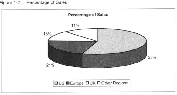
Shoe Co. manufactures and distributes products including athletic shoes, sportswear, sports accessories, men's casual wear, casual shoes, and apparel. The US is its major market. According to its 2004 annual report, the US market accounts for 55% of sales, Europe for 21%, the UK for

13%, and other regions for 11% (Figure 1-2).

Figure 1-2 Percentage of Sales

Percentage of Sales 11%

13/

55%

[PUS KEurope OUK 0 Other Regions

Moreover, in 2004, footwear products were the most important business, accounting for 64% of sales while apparel products account for 36%. Footwear products account for around 60% to 70% of the business in North America.

In summary, the footwear products in the US market are the focus according to Shoe Co.'s strategy. Thus, the scope of the DC bypass project focuses on the US market of footwear products.

(11)

1.2.1 Current Logistics Operation

In this section, we provide an overview on Shoe Co.'s logistics network.

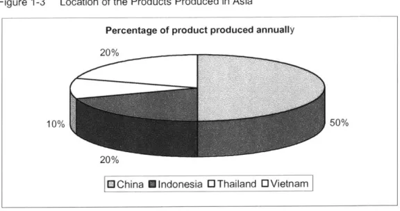
Shoe Co. currently manufactures all of its footwear products in Asian countries including China, Indonesia, Thailand, and Vietnam. As shown in Figure 1-3, Chinese manufacturers account for the majority of the manufacturing, producing on average 50% of the footwear products annually. Indonesia and Vietnam manufacturers account for 20% of the production each, while Thailand manufacturers account for 10%. After manufacturing, the finished products are loaded in forty foot unit (FEU) containers at the factories, transported via ocean carriers, and shipped to the markets.

Figure 1-3 Location of the Products Produced in Asia

Percentage of product produced annually

10% 50%

20%

SChina Mindonesia OThailand OVietnam

Table 1-1 shows the locations of major plants and export ports Shoe Co. employs in Asia. However, in this project, we do not assume that we export cargo from all of the listed ports. We will explain the reason why we make this assumption in Chapter 3.

(12)

Table 1-1 Percentage of the Products Produced in Asia

Country City Port

China Shenzhen Hong Kong, Shekou, and Yantian

Fuzhou Fuzhou and Fuqing Zhuhai Hong Kong

Indonesia Jakarta Jakarta Thailand Bangkok Bangkok

Vietnam Ho Chi Minh City Ho Chi Mihn City

Shoe Co. classifies customer's orders into two categories: full-container-load (FCL) and less-than-container-load (LCL) orders. Products for FCL orders are shipped directly to customer locations after arriving at the US. These orders are out of the scope of the DC bypass project. Products for LCL orders are processed at the Stoughton DC. In general, 60% of the footwear orders are regarded as FCL orders while the other 40% are LCL orders. The final destinations of LCL-order products are decided either at the Asia factories (50%-60%) or during the ocean transit (40%-50%).

After manufacturing, products for LCL orders are loaded into containers and shipped from the Asian ports via ocean carriers to the US. There are two shipping routes: all-water and mini-land bridge. The all-water route passes through Panama Canal and arrives at the East coast of the US at ports in New Jersey, New York, Baltimore, or Savannah. The mini-land bridge route arrives West Coast ports such as Seattle or Long Beach. After arriving at the US ports, LCL-order containers are shipped to the Stoughton DC. Containers moving via the all-water route are

shipped by trucks while those via mini-land are shipped by intermoda 2 or long haul3_{. After cargo}

arrives at the Stoughton DC, value-added activities, such as price tag labeling, are performed. The largest customers for Stoughton DC are Shoe Co.'s own retailers. When placing orders to

2 The use of at least two modes of transportation to complete a shipment such as truck/rail/ or ship/air.

(13)

the Stoughton DC, customers arrange routing from the distribution center to their warehouses and pay for transportation costs.

1.3 Scope of the Distribution Center (DC) Bypass Project

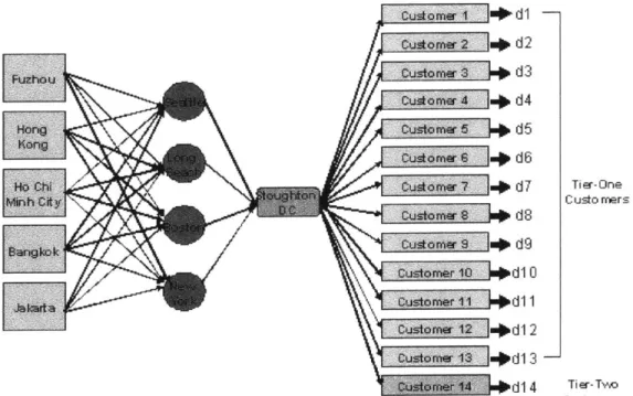
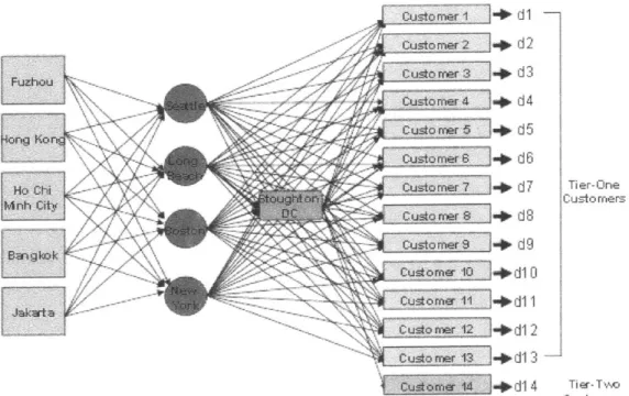
Figure 1-4 displays the existing network, a four-echelon distribution network which includes five departure ports in Asia, four entry ports in the US, a distribution center in Stoughton, hereafter called the Stoughton DC, and customers' locations. Before explaining the figure, we want to stress again that the network displayed in Figure 1-4 is the simplified compared to Shoe Co.'s actual supply chain. We will state the reasons why we simplified it in Chapter 3.

Figure 1-4 Existing Footwear Supply Chain

i;toe a Wd1 -dl 4 cuge2 .d2 cuitoaery .# d3 cuame 4 N d Custamer 6 Hyd7 Customer 710 V1 Csormer 11 4d11 Customer 12 Id1 2 cusdome 1 Id13-d1 4 Tier-One Custo mers Tier-Tvo Customers FUzho u Kong Ho J:W it O'e,

(14)

In Figure 1-4, the left nodes represent the location of five departure ports: Fuzhou, Hong Kong, Ho Chi Minh City, Bangkok, and Jakarta. Shoe Co. exports its footwear product via ocean carriers through these five ports to the US market. As we mentioned before, it is a simplified network and thus not all Asian ports are assumed to use in our project. In this case, we use Fuzhou to represent all of the Chinese ports and the reason will be stated in Chapter 3.

There are four potential arrival ports: Seattle, Long Beach, Boston, and New York. These four entry ports are also considered for hosting the DC bypass operation. Thus, these four entry ports will potentially serve as both arrival ports and DC bypass locations.

The Stoughton DC is used in the existing logistics network. It performs traditional

warehousing functions including receiving, putting away, storage, picking, and handling. In the DC bypass project, we suggest customers be separated into two tiers. All or some Tier-One Customer orders will be served by shipping products directly to the customers' locations.

The right nodes in Figure 1-5 represent the locations of customers. All customers, which are served by the Stoughton DC, are aggregated into two groups: Tier-One and Tier-Two. Tier-One Customers are represented by specific end locations, usually their distribution centers. Only Tier-One Customers may participate in the DC bypass network. All other customers are classified as Tier-Two Customers and will not participate in the DC bypass network. That is, even if the DC bypass is implemented, Tier-Two Customers will still be served by the Stoughton DC although the exact flow pattern through the network will be determined by the model.

(15)

Figure 1-5 Potential Footwear Supply Chain Fuzhou Ho Chi M nh City 76 Customer + d1 Z, Customn-er 2 J- d 2 cu worer 3 1- d 3 Customer 4 * d 4 C ustomr 5 +d5 custom-r 6 d6 40staer 7 * d7 Tier-One Customers - Custo mrer 8 a* d8 Cu-zo Mr 9 d9 Customer 10 *d1 0 C usto m-er 12 +d1 2 C usto ror 13 J- d1

3-tIZ4 oM - 1 d4 4 Tier- T*,o

Customers

As shown in Figure 1-5, the DC bypass project converts the three echelon network into a two echelon network for selected items: departure ports to entry ports, then directly on to a customer. After products for Tier-One Customers arrive at an entry port, they are shipped from directly to Tier-One Customers' location or to the Stoughton DC and then onto the customer's location. There are thirteen Tier-One Customers. In Figure 1-5, d denotes annual demand. dl to d13 represents the One Customer annual demand which is satisfied by Shoe Co.. All Tier-Two Customers' orders are aggregated into one group, Customer 14, in our model because these

orders all destine at the Stoughton DC and the customer pays for the transportation for the Stoughton DC to their distribution centers.

Through the DC bypass project, Shoe Co. expects a reduction in total costs. Possible benefits will be discussed and identified.

(16)

Methods to determine a specific location or multiple locations for the DC bypass operations will be discussed. Furthermore, the robustness of the optimal solution will be measured through a sensitivity analysis.

Other benefits from the DC bypass project include the reduction of lead time but we will not cover this topic in this thesis. Intuitively, the lead time from the arrival port directly to the Tier-One Customers' locations will be less than that of the routing through the Stoughton DC because the latter includes the processing time in the Stoughton DC. We will discuss this topic in Chapter

5 for the further research.

In summary, through the DC bypass project, we want to answer the following questions:

1. Should the DC bypass be implemented to minimize the total supply chain costs?

2. If the DC bypass should be implemented, should we implement it for all Tier-One Customers' orders or some of them?

3.What location should be chosen to implement the DC bypass operation?

4. Should we choose one port or multiple facilities for the DC bypass?

5. How many Tier-One Customers' order should go through these entry ports?

6. How does the network solution vary with different costs? For example, if the capital cost to set up a facility for DC bypass operation decrease, will any port become more

desirable? How does the optimized result vary if a DC bypass handling cost change?

The remainder of this thesis is organized as follows. Chapter 2 discusses previous

(17)

explains the source of data and summarizes the data and assumptions. Chapter 4 presents the mixed integer linear programming model used in the analysis. Finally, Chapter 5 reviews the analysis and recommends further research.

(18)

2 Literature Review - Methodologies and Case Studies

This chapter summarizes commonly used methodologies for the network design problem. Moreover, we refer to previous case studies similar to our project to illustrate these methodologies.

2.1 Minimum Cost Flow Problem

Hillier and Lieberman (2005) note that network analysis is used in many areas including communication, electricity, and transportation. Furthermore, there are many basic prototypes of network problems such as the shortest path problem, the minimum spanning tree problem, and the maximum flow problem. The most commonly applied problem in the network analysis is the minimum cost flow problem. The problem converts a network into the configuration of nodes and links. For example, in a logistics network, nodes are the locations of facilities; links, also called arcs, are transportation movements between facilities. Costs of activities occurring at nodes and arcs are expressed by momentary units such as dollars. For example, when footwear products are shipped by an ocean carrier from Asia to the US, the transportation is expressed by the ocean freight spent on this activity.

Minimum Cost Flow Problems can be formulated and solved by mathematical programming such as linear and mixed integer linear programming. According to Shapiro (2001),

mathematical programming models are 'venerable' studies in the field of operations research since the 1950s. They can help managers to make supply chain decisions including network design problems. Linear programming and mixed integer programming can be used in all types

(19)

of supply chain decisions. They can produce analyses of a system (e.g. a logistics network) with the goal of maximizing or minimizing an objective function subject to constraints, e.g., the maximization of profit given a budget constraint on marketing and production. A study for Citgo Petroleum Corporation (Klingman, Phillips, Steiger, & Young, 1987) is a typical example of applying the minimum cost flow method to improve a company's supply chain. The company developed a linear-programming-based network optimization model that reduced inventory by $116 million. In brief, network design problems can be regarded as minimum cost flow

problems, which can be solved by optimization method such as linear programming.

The difference between linear and mixed integer linear programming is that the former assumes all variables are continuous whereas the later suppose some variables are continuous while others are integers. The decision variables of mixed integer linear programming can be both the output of products at and among facilities, and binary variables, which decide whether to open a facility. The objective in a network design problem is typically a minimization of total supply chain costs given five major constraints: capacity constraints, customer services goals (e.g. 99.97% fill rate), logical constraints (e.g. if a facility is built, it must have a product flow), balance constraints (e.g. the number of products moving into a location is equal to the number of products moving out), and demand constraints (all customer demand must be served).

Overall, network design problems are complicated because there are many trade-offs in network design problems. Mathematical programming can help to find the best balance between the trade-offs. For example, an increase in the number of warehouses decreases outbound transportation costs but increases inventory and facility costs. The method can determine how many warehouses to be set to minimize total costs including transportation, inventory, and facility costs. In the mid- 1 990s, Sery, Perst, and Shobrys (2001) described how BASF North

(20)

America, a global chemical company, examined its distribution network. BASF faced conflicting objectives of minimizing transportation costs while improving customer service goals. The costs

included fixed costs to run a distribution center, variable handling, inventory costs, and

transportation costs. The service was measured by same-day and next-day delivery. Therefore, by using linear programming, Sery at el. (2001) helped BASF's management find a balance between the trade-offs. BASF decided to open a new warehouse according to this analysis and

increased the volume of goods delivered next day by fifteen percent.

In addition to mathematical programming techniques, Chopra and Meindl (2003) also suggest the use of a gravity model, a mathematical technique used to find the best location of a facility, say, a distribution center, which minimizes distribution costs. The method assumes the locations of facilities are on a Cartesian co-ordinate system in which the origin and the scale in the system is user-defined. It also premises that transportation costs are directly proportional to both distance and volume shipped and that the distance is weighted by the volume of products. The optimal location is that, which minimizes the weighted distance between the facility and the markets.

While the gravity method is easy to solve, it may not lead to a feasible location and tends to oversimplify the problem. For example, supposed a company wants to decide where to locate a warehouse. The result of a gravity model may suggest the best location to minimize the

distribution cost is a place at Longitude 41-53'l 8" N and Latitude 087-36'08" W, which is the location of Lake Michigan! Also, the gravity model assumes that all facilities are open. Thus, optimization method is better than the gravity method for our project because it shall not suggest an infeasible location and consider not just distribution costs but total supply chains costs.

(21)

2.2 Baseline, Optimization, and Simulation Models

To derive an optimal solution for a network design, Levi, Kaminsky, and Simchi-Levi (2004) suggest a two-step procedure. First, a company should develop a baseline model representing its current logistics network. Then, based on the validated baseline model, the company should build another model to find a feasible solution such as a cheaper or more responsive network by dispatching facilities such as distribution center candidates. They suggest using one of two methodologies: optimization or simulation.

We have already described exact optimization techniques using mixed integer linear programming methods. In addition to exact approaches, there is a whole family of heuristics techniques. Heuristics methods find good but not necessarily optimal solutions. There are two reasons for a company to use heuristics. First, as the size of a network problem increases, it is more difficult to get a feasible solution by exact algorithms. Heuristics can help find a better starting solution for exact methods. Second, heuristics are much faster and are easier to explain.

While optimization is typically used to deal with static information, simulation captures stochastic or random data. Simulation is a process of modeling the random features of a system and then making repeated runs to uncover likely results. It is used to model dynamic systems or systems that are too analytically complex for optimization. For example, suppose that customer demand follows a normal distribution and affects the profits, we can simulate how the profits changes as the demand randomly changes. The requirements of a good transportation network vary with several factors. For example, if demand is concentrated in a certain area, a centralized warehouse tends to be more adequate than multiple warehouses. Simulation can be used to capture the dynamics of a logistics system. However, simulation cannot determine the best

(22)

network but, rather, can evaluate or score each network configuration. For example, we can develop two logistics network: one has a centralized warehouse while other has multiple

warehouses. Then, we can see how supply chain costs vary with the demand under two different logistics network. Then, the managers can choose the better one. In brief, simulation is a tool for the management to select between a set of options, which is not necessarily optimal.

2.3 Conclusion

For many years, these optimization methods have been applied by many companies such as BASF, Citigo, and HP as the above cases showed. Linear-programming-based and mixed-integer-programming-based optimization models are the most commonly used tools in network design problems. Mixed integer programming is a better tool to formulate our project because we need a model to determine the flow of products at the network (continuous variables) and to decide which entry port is used to import the products and open a facility for the DC bypass operations (binary variables). The mixed-integer-based model is used in many case studies. Arntzen, Brown, Harrison, and Trafton (1995) developed a mixed-integer linear program, called the Global Supply Chain Model for Digital Equipment Corporation (DEC). The model

represented DEC's distribution, production, and vendor network and helped management redesign DEC's network and saved over $100 million accordingly. We will use mixed integer programming to formulate and solve our problem for this project.

(23)

3 Data

As Chapter 2 revealed, we can solve network design problems by using a mixed-integer-linear-programming-based optimization model. This requires a large amount of data, however. In Section 3.1, we will explain the source of the data. In reality, it may not be possible to collect all of the data we need. Therefore, we also need to make assumptions to extract the information we need from the data we actually collect. For example, we need to know port handling charges, but typically door-to-door4 ocean charges are provided. We have to make assumptions to extract port handling charges from the total costs. In Section 3.2, we will summarize the data we collect and describe the assumptions.

Most of the data are from Shoe Co. However, to protect the privacy of Shoe Co., we have changed or modified data based on particular principles, which will be described later.

3.1 Sources of Data

The model required a large amount of both qualitative and quantitative data. First, we conducted interviews to create a qualitative description of the operation of Shoe Co.'s transportation

network. Then, through weekly meetings starting in February, data and the existing network map were validated. Moreover, transactional data was collected from Shoe Co.'s for us to understand

4 Door to door refers to the through-transport of goods from a shipper to a consignee. Door-to-Door transportation usually includes multiple modes such as vessels, trucks, or air in one shipment. Many ocean carriers provide door-to- door service to satisfy customers' demand.

(24)

the demand pattern. No data is based on future forecasts except the average number of shoes per container in 2005.

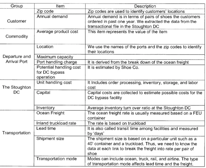
All data can be classified into the following groups: customers, commodity, departure and arrival ports, the Stoughton DC, and transportation (Table 3-1). We will illustrate the data we collect and how we make assumptions based on it in Section 3.2.

Table 3-1 Data Collection List

Group Item Description

Zip code Zip codes are used to identify customers' locations

Annual demand Annual demand is in terms of pairs of shoes the customers Customer ordered in past one year. We extracted the data from the

transactional file in the Stoughton DC

Average product cost This item represents the value of the item Commodity

Location We use the names of the ports and the zip codes to identify their locations

Departure and Maximum capacity

Arrival Port Port handling charge It is derived from the break down of the ocean freight Potential handling cost It is estimated by Shoe Co.

for DC bypass

operation

Unit handling cost It Includes order processing, inventory, storage, and labor

The Stoughton cost

DC Capital Capital costs are collected to estimate possible costs for the

DC bypass facility

Inventory Average inventory turn over ratio at the Stoughton DC Ocean Freight The ocean freight rate is usually measured based on a FEU

container

Inland truckload rate The rate is based on truckload

Lead time It is also called transit time among facilities and measured

Transportation by 'days'

Shipment size The shipment size is based on a particular unit such as a 40' container and a truckload. Thus, we need to know the data at each link to break the freight into rate per pair of shoe

Transportation mode Modes can include ocean, truck, rail, and airline. The type of transportation mode affects lead time and the freight.

(25)

3.2 Data and Assumptions

In reality, there are over 300 different combinations of routings to ship product from Asia to a customer location. However, we do not build a model based on these combinations but a simplified model. For example, as we mentioned in Chapter 1, we do not assume that we export cargo from all ports Shoe Co. uses now because the DC bypass project is evaluated for selected customers, Tier-One Customers, and thus Shoe Co. chooses major ports to import and export products to aggregate the flow of the products. The aggregation will not hurt the accuracy of the model and we will validate the accuracy in Chapter 4. Moreover, the aggregation by adequately choosing major ports can decrease the complexity of the formulation and consequently reduce the solver time and get a feasible solution more easily. Therefore, we decide to analyze and optimize the network based on a simplified logistics network.

Before optimizing the network, we need to make certain assumptions. The assumptions are as follows:

3.2.1 Commodity

We assume that products are shipped via FEU containers at sea and via a truckload on land. Moreover, to build the optimization model, we need to break the freight into transportation cost per pair of shoes at each link. Therefore, we should know the average numbers of shoes a FEU container and a truckload can hold. According to Shoe Co., the shipment size averages between 6,000 to 6,500 pairs per FEU container. Table 3-2, based on forecasts and historic data, shows the average number of shoes per container for 3 years. In this project, we refer to the average number, 6,171 pairs of shoes, in 2005 to break the door-to-door- ocean rates.

(26)

Table 3-2 Average Pairs of Shoes per FEU Container

Year Units per FEU Container

2003 6,393

2004 6,150

2005 6,171

Moreover, we focus on the basic cost unit is cents per pair.

1.5 pound and account for 0.39

annual flow of finished goods, modeled as pairs of shoes. The According to Shoe Co., each pair of shoes is assumed to weigh cubic feet.

3.2.2 Breakdown of the Ocean Freight

For the modeling, we need to know the following costs in terms of cents per pair of shoe: handling cost at departure and arrival port, port-to-port5 ocean freight, and inland transportation rate for the shipment from then US entry port to the Stoughton DC. These costs are included into the door-to-door ocean freight. The freight rate per FEU container includes the bunker6

adjustment factor7 and security fees'. Then, we need to figure out a reasonable assumption to break the door-to-door freight into a cost per unit.

Table 3-3 displays the average ocean freight costs. According to the agreement between Shoe Co. and its ocean carriers, Shoe Co. cannot reveal its rate to other organizations. Therefore,

5 Port-to-port denotes the transport of goods via an ocean route from a departure port to an arrival port. 6 Bunker is a fuel for ships to sail.

7 Bunker adjustment factor refers to a fee for adjustment applied by shipping carriers to offset the effect of fluctuations in the cost of bunkers.

' There two types of security fees: Terminal Security Fee, charged for the shipments via the ports where the threat

and the need for increased security are based on a realistic threat; Carrier Security Fee, based on ongoing costs to keep ships and the crew secure.

(27)

to avoid breaking the agreement, Shoe Co. provided us the rate quoted by one of the ocean carriers it hires without revealing the carrier's name.

Shoe Co. pays for the door-to-door ocean freight from Asia to the Stoughton DC in the existing network. The basic unit of the door-to-door rate is a FEU container.

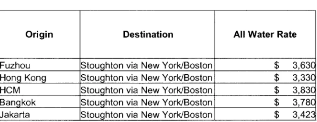
In the existing network via all-water routes, the arrival ports are either Boston or New York. Moreover, the door-to-door freight rate, as presented in Table 3-3, is the same regardless of the arrival port.

Table 3-3 Door-to-Door All-Water Ocean Freight

Origin Destination All Water Rate

Fuzhou Stoughton via New York/Boston $ 3,630

Hong Kong Stoughton via New York/Boston $ 3,330 HCM Stoughton via New York/Boston $ 3,83C

Bangkok Stoughton via New York/Boston $ 3,78C

Jakarta Stoughton via New York/Boston $ 3,423

To break down the door-to-door ocean rate into cost per unit, we refer to Saanen's research in 2004 (Table 3-4). The door-to-door ocean freight rate consists of different costs for activities such as inland transportation, port handling, and sea shipping. For example, Sannen asserts that 33% of the door-to-door ocean freight costs are due to sea shipping (port to port) costs.

Percentages for other activities such as port handling are displayed in Table 3-4.

Table 3-4 Average Share of Ocean Freight

Inland Truck in Departure Port Arrival Port Truck/Rail in

the Origin Handling Sea Shipping Handling the Destination Total

Country Country

(28)

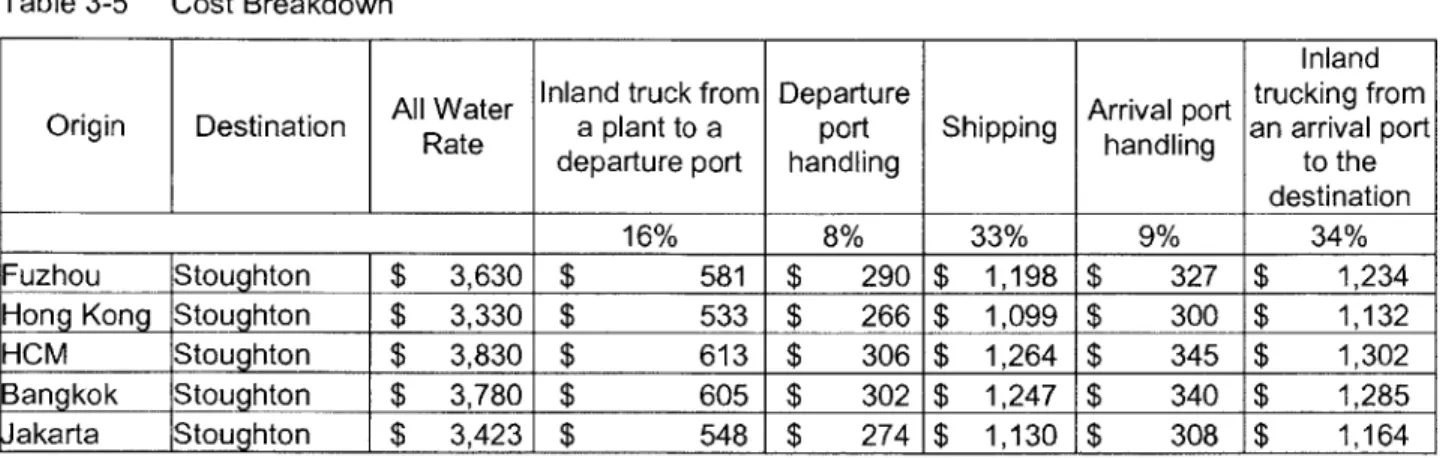
Then, as listed in Table3-5, we get the following costs by using Shoe Co.'s freight times a certain percentage derived from Table 3-4. The arrival port is Boston or New York.

Table 3-5 Cost Breakdown

Inland

All Water Inland truck from Departure Arrival port trucking from

Origin Destination Rate a plant to a port Shipping handling an arrival port

departure port handling to the

destination

16% 8% 33% 9% 34%

Fuzhou Stoughton $ 3,630 $ 581 $ 290 $ 1,198 $ 327 $ 1,234

Hong Kong Stoughton $ 3,330 $ 533 $ 266 $ 1,099 $ 300 $ 1,132

HCM Stoughton $ 3,830 $ 613 $ 306 $ 1,264 $ 345 $ 1,302

Bangkok Stoughton $ 3,780 $ 605 $ 302 $ 1,247 $ 340 $ 1,285

Jakarta Stoughton $ 3,423 $ 548 $ 274 $ 1,130 $ 308 $ 1,164

Per our assumption, the port handling charge is the same in Boston as in that in New York. Therefore, it is not reasonable for us to have a arrival port handling cost ranging from $300 to $340. Therefore, we decided to unify the handling cost at an arrival port by averaging the arrival port handling costs listed in Table 3-5, that is, $324. Then, we readjust the ocean shipping rate by modifying the number accordingly as shown in Table 3-6.

Table 3-6 Adjusted Cost Breakdown

Inland

. All Water Inland truck from Departure Adjusted Arrival port trucking from Origin Destination Rate a plant to a port Shipping handling an arrival port

departure port handling to the

destination

Fuzhou Stoughton $ 3,630 $ 581 $ 290 $ 1,201 $ 324 $ 1,234

Hong Kong Stoughton $ 3,330 $ 533 $ 266 $ 1,075 $ 324 $ 1,132

HCM Stoughton $ 3,830 $ 613 $ 306 $ 1,285 $ 324 $ 1,302

Bangkok Stoughton $ 3,780 $ 605 $ 302 $ 1,264 $ 324 $ 1,285

Jakarta Stoughton $ 3,423 $ 548 $ 274 $ 1,114 $ 324 $ 1,164

Likewise, we also get the share of ocean freight for the mini-land route from Asia to Long Beach and Seattle as listed in Table 3-7.

(29)

Table 3-7 Adjusted Cost Breakdown According to a Particular Ratio

All Water Inland truck from Departure Adjusted Arrival port Origin Destination Rate a plant to a port Shipping handling

departure port handling

Fuzhou Seattle $ 2,900 $ 581 $ 290 $ 1,770 $ 259

Hong Kong Seattle $ 2,700 $ 533 $ 266 $ 1,642 $ 259 HCM Seattle $ 2,800 $ 613 $ 306 $ 1,622 $ 259

Bangkok Seattle $ 3,000 $ 605 $ 302 $ 1,834 $ 259

Jakarta Seattle $ 3,000 $ 548 $ 274 $ 1,919 $ 259

Fuzhou Long Beach $ 2,900 $ 581 $ 290 $ 1,770 $ 259 Hong Kong Long Beach $ 2,700 $ 533 $ 266 $ 1,642 $ 259 HCM Long Beach $ 2,800 $ 613 $ 306 $ 1,622 $ 259

Bangkok Long Beach $ 3,000 $ 605 $ 302 $ 1,834 $ 259 Jakarta Long Beach $ 3,000 $ 548 $ 274 $ 1,919 $ 259

From Section 3.2.1, we know that average number of shoes in a FEU container is 6,171. Therefore, we can convert the above costs into costs per pair of shoes by dividing the costs by

6,171. Then, we can get unit ocean shipping rate for the replenishment link. Take shipping costs

from Fuzhou to Seattle for example, the unit shipping rate is 29 cents per pair of shoes.

3.2.3 Link- Replenishment, Inland Transportation, the DC bypass, and Outbound

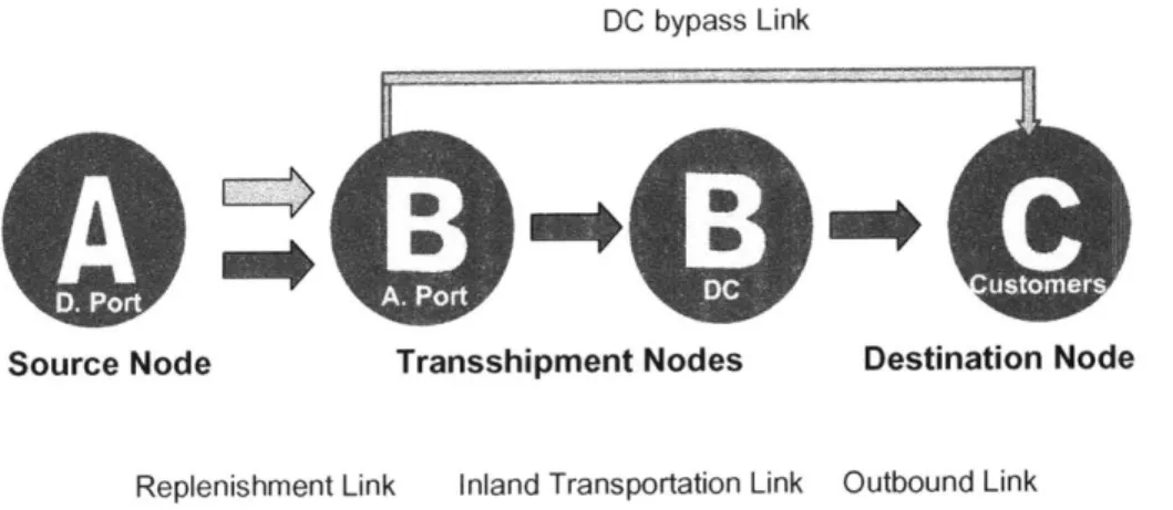
As shown in Figure 3-1, There are four types of links in our analysis: replenishment, inland transportation, the DC bypass, and outbound. Replenishment links represent shipments between Asian departure ports and the US arrival ports. Inland transportation links identify the

distribution between arrival ports and the Stoughton. Outbound links capture the transportation, paid by the customers, from the Stoughton DC to Tier-One Customers' locations. DC bypass link is similar to the outbound link. It represents the shipments from the arrival ports to the Tier-One Customers' locations but the transportation costs are paid by Shoe Co..

(30)

Figure 3-1 Links in Shoe Co.'s Supply Chain

DC bypass Link

Source Node Transshipment Nodes Destination Node

Replenishment Link Inland Transportation Link Outbound Link

In summary, there are two flows in Figure 3-1. One is the flow of products in the existing supply chain network. They depict the flow of finished products in the existing three-echelon network including departure ports, arrival ports, Stoughton DC, and customers. The other is the

flow of products in the DC bypass network, a two-echelon logistics network including departure ports, arrival ports, and customers.

Replenishment Link

In general, ocean contract rates are confidential and can only be issued with the carrier's permission to the third party. Therefore, as we mentioned in the beginning of the chapter, all rates are real without knowing the carrier's name.

The majority of Shoe Co.'s product is shipped via full containers from the factory. Very few of them are transloaded at the port. Transloading is the process of transferring a shipment from one mode of transportation to another. It usually refers to an operation to discharge cargo from a container on a rail car to a truck, and then eventually delivered to the customers' door by a truck. The reason why transloading is performed is for the benefit of economies of scale because the

(31)

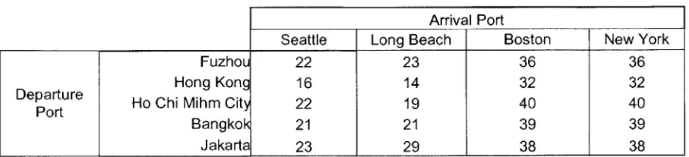
Table 3-8 shows the lead time (days) from Asian ports to the US ports. Though the purpose of this project is to seek the least cost solution, the data can be used in the further research, which includes a consideration of the lead time.

Table 3-8 Lead Time (day) at Replenishment Link

Arrival Port

Seattle Long Beach Boston New York

Fuzhou 22 23 36 36

Hong Kong 16 14 32 32

Departure Ho Chi Mihm City 22 19 40 40

Bangkok 21 21 39 39

Jakart 23 29 38 38

Inland Transportation Link, DC bypass Link, and Outbound Link

Truckload transportation rates were based on $2 billion of total truckload movements. A regression of this freight resulted in an estimated cost function. The resulting equation is $262 +

$1.05*Distance (mile). By this equation, we derive unit rate (cent) for inland transportation and the DC bypass link (Table 3-9 and Table 3-10). Distribution at inland transportation link is paid by Shoe. Co while the outbound transportation rate from the Stoughton DC to a customer is paid by the customer. Therefore, in the model, we assume that the unit rate from the Stoughton DC to

customers' location is zero (Table 3-10).

Table 3-9 Unit Transportation Rate at Inland Transportation Link The Stoughton DC

Seattle 36.30

Arrival Port Long Beach 37.67

Boston 3.51

(32)

Table 3-10 Unit Transportation Rate at Inland Transportation and Outbound Link Tier-One Customer Seattle 38.6 27.4 20.1 31.4 35.1 27.4 31.6 44.1 43.9 40.6 39.0 20.2 20.2 Long Beach 33.9 24.6 4.3 24.0 26.3 24.6 24.1 42.9 44.8 36.4 36.1 4.3 4.3 Bostor 21.5 26.7 46.8 30.1 31.0 26.7 30.2 11.8 7.1 19.7 17.6 47.1 47.0 New York 18.4 24.2 44.3 27.2 28.0 24.2 27.3 8.9 4.3 16.6 14.5 44.7 44.6 Stoughtor - - T - - - - - - -

-Likewise, though we do not use the data about the lead time, we still collect the data for the further research in Chapter 6 (Table 3-11 and Table 3-12).

Table 3-11 Lead

Table 3-12

Time (day) at the DC Transfer Link

Lead Time (day) at DC Transfer and Outbound Link

Tier-One Customer Seattle 5 4 3 4 5 4 4 5 5 5 5 3 3 Long Beach 4 4 1 3 3 4 3 5 4 4 4 1 1 Boston 3 4 4 4 4 4 4 2 1 3 3 4 4 New York 3 3 4 4 4 3 4 2 1 3 3 4 4 152u6 3 4 5 7 10 11 12 13 Stoughtonj 3 4 4 4 4 4 4 2 1 3 3 -4 4

3.2.4 Ports- Departure and Arrival

In this section, we discuss the data about the port data and the underlying assumptions.

DC Transfer The Stoughton DC

Seattle 5

Arrival Port Long Beach 4

Boston 1 New York 1 6 7 8 1 2 3 4 5 9 10 11 12 13 6 7 8 1 2 3 4 5 9 10 11 12 13

(33)

Departure Ports

Shoe Co. manufactures all shoes in Asia at factories near one of the departure ports, which are Fuzhou, Hong Kong, Ho Chi Minh City, Bangkok, and Jakarta. We assume that Shoe Co. exports its footwear product through these ports to the US market. According to Shoe Co.'s historic data for the last year, each port accounts for 20% of the total export volume as shown in Table 3-13. In our model, the percentage at the departure ports is fixed at this historic level. That is, in this project, the choice of the departure ports is not the decision we would like to make because we assume products are exported from Asia based on the percentage presented in Table 3-13. Moreover, the number of units also represents the maximum throughput at each port.

Table 3-13 Historic Export Volume at a Departure Port

Departure Port Unit Percentage

Fuzhou 4,350,990 20%

Hong Kong 4,350,990 20%

Ho Chi Mihm City 4,350,990 20%

Bangkok 4,350,990 20%

Jakarta 4,350,990 20%

Total 21,754,950 100%

Moreover, we do not assume other costs except port handling costs at departure ports as shown in Table 3-14, which are derived from door-to-door ocean rate as we illustrated earlier in this chapter.

Table 3-14 Handling Cost at a Departure Port

Cent/Unit

Fuzhou 4.70

Hong Kong 4.31

Ho Chi Mihm City 4.96

Bangkok 4.89

(34)

Arrival Ports and Candidates for the DC bypass Operation

In practice, Shoe Co. imports cargo via the US entry ports including Seattle, Tacoma, Long Beach, Houston, Miami, Charleston, Savannah, Norfolk, New York, Boston, and Halifax. Shipments arriving at Halifax are shipped on a feeder ship to Boston.

However, in our project, we assume that we import cargo via Long Beach, Seattle, Boston, or New York because we focus on Tier-One Customer orders and above ports are major entry ports for these customers. Moreover, all shipments to customers are via truck.

According to Shoe Co.'s historic data, each arrival port processes a certain percentage of the import volume (Table 3-15). The number of units also represents the maximum throughput at each port in our modeling. This maximum throughput, worked as the higher bound in the mixed integer linear programming, is used as a capacity constraint.

Table 3-15 Historic Import Volume at an Arrival Port

Arrival Port Unit Percentage

Seattle 1,087,748 5%

Long Beach 5,438,738 25%

Boston 870,198 4%

New Yorkj 14,358,267 66%

Total 21,754,950 100%

A capacity constraint is applied because of a risk issue. Few companies import products through one port because of the concept of portfolio. For example, suppose Shoe Co. imports all products via Long Beach in the peak season. If there is a congestion or strike in Long Beach, the transit time will increase and hurts Shoe Co.'s business because it cannot meet the demand of the peak season.

(35)

However, we may assume there is no capacity constraint under some scenarios to examine whether releasing the capacity constraint can cause savings in total supply chain costs and how the reallocation of the import volume affects the solutions.

Table 3-16 reveal possible unit handling cost for the DC bypass operation. The cost is estimated by Shoe Co. for the DC bypass network. Therefore, we need to conduct a sensitivity analysis to reveal how the change in this cost will affect the optimal results.

Table 3-16 Handling Cost for the DC Bypass Operation Handling for the DC Cent/Unit

bypass operation Cent/Unit

Seattle 5

Long Beach 5

Boston 5

New York 5

3.2.5 Stoughton Distribution Center

Shoe Co. actually has two DCs. A bigger one is at Stoughton while a smaller one is at Norwood. However, Shoe Co. employs one warehouse management system to operate both warehouses. The system regards two DCs as one DC in its database, Therefore, the transactional files we collected assume there is only one DC which serves Shoes Co.'s customers. Therefore, we premise that there is only one DC, the Stoughton DC, in the existing logistics network.

The new network will bypass the Stoughton DC. Now all footwear products of LCL orders are shipped to Stoughton DC directly after arriving at the entry ports in the US. In the DC bypass network, all or some Tier-One Customer orders will bypass the Stoughton DC. That is, if the DC bypass is implemented, related costs accruing in the Stoughton SC will be eliminated while other DC bypass costs will incur.

(36)

Inventory

Average inventory at the Stoughton DC is 4.1 million with an average inventory turnover ratio of four. That is, inventory stays in the Stoughton DC for 3 month on average. However, because our focus is on the minimization of total supply chain cost, not the lead time issue, we will not

include this data in our analysis.

Handling Cost

Average handling cost in the Stoughton DC is $0.92 per pair. This cost includes inventory, order processing, and labor costs.

Facility Cost

Capital cost of the Stoughton DC is $2.5 million while Norwood is $1.6 million. We need this information to estimate facility cost for DC bypass project. The higher the facility cost, the lower the chance the optimization model would suggest multiple locations for a DC bypass. In some initial models, we assume that it costs $2 million (the rough average of $2.5 and $1.6 million) if we build a new facility for the DC bypass project. However, this estimation may be too high because of two reasons: 1) the volume of products is less than the throughput at Stoughton DC because only some of the customers will participate this project; 2) Shoe Co. may hire a third party logistics firm to handle the DC bypass operation and thus may not have fixed costs. Due to the above reasons, we will conduct sensitivity analysis on facility costs to see how they impact the solution. The related analysis will be discussed in Chapter 5.

(37)

3.2.6 Customers

From the transactional file Shoe Co. provided, we can rank the top 13 customers according to order quantity in the past year as shown in the Table 3-17.

Table 3-17 Top 13 Customers

Rank Shipment Quantity %

1 4,497,813 21% 2 857,774 4% 3 744,678 3% 4 744,565 3% 5 652,326 3% 6 502,499 2% 7 485,674 2% 8 420,561 2% 9 400,905 2% 10 360,926 2% 11 353,941 2% 12 340,391 2% 13 325,398 1% Total 21754950 100%

However, not all of these customers are candidates for the DC bypass project. Customers are classified into two tiers. Customers, which are served by Stoughton DC, are aggregated into two groups: Tier-One Customers and Tier-Two Customers. Tier-One Customers are represented by specific end locations, usually their distribution centers. Only Tier-One Customers may

participate in the DC bypass network. Shoe Co. chose DC bypass partner based the following criteria: 1) potential order quantity in the future; 2) general order pattern; 3) ease and willingness to join the DC bypass project; and 4) the location of customers. Table 3-18 summarizes the order quantity of 13 potential customers for this DC bypass customers. These customers, Tier-One Customers, account for 26% of order quantity shipping from Stoughton DC.

(38)

Table 3-18 Tier-One Customers in the DC Bypass project

Demand Weight Demand Demand % of Total

Customer Customer Location Demand (Units) (Pounds) (CWT9) (CFT") Volume

1 Birmingham, AL 353,946 530,919 5,309 137,082 2% 2 Junction City, KS 400,905 530,919 6,014 155,269 2%

3 West Puente Valle, CA 360,926 601,358 5,414 139,785 2% 4 Haslet, TX 652,326 541,389 9,785 252,643 3% 5 Katy, TX 485,674 978,489 7,285 188,099 2% 6 Junction City, KS 260,996 728,511 3,915 101,083 1% 7 Fort Worth, TX 744,678 24,280,812 11,170 288,410 3% 8 Newport News, VA 325,398 1,117,017 4,881 126,025 1% 9 Bronx, NY 502,499 488,097 7,537 194,616 2% 10 McDonough, GA 744,565 753,749 11,168 288,367 3% 11 Whites Village, TN 156,565 1,116,848 2,348 60,637 1% 12 Watts, CA 238,873 234,848 3,583 92,514 1% 13 Downey, CA 340,391 358,310 5,106 131,832 2%

We find that these locations of Tier-One Customers correspond to Top 10 Cities, where the major destinations of orders served by the Stoughton DC in the past one year (Table 3-19). These orders include the demand from both Tier-One and Tier-Two Customers.

Table 3-19 Top 10 Cities

To 10 Cities with the Largest Annual Volume

City Zi Shipment Quantit % of Total Volume

Junction City, KS 66441 1,175,556 5.10% Bronx, NY 10461 504,248 2.19% Katy, TX 77449 485,674 2.11% Haslet, TX 76052 447,380 1.94% Carlisle, PA 17013 417,613 1.81% Birmingham, AL 35211 351,309 1.52% Evansville, IN 47725 293,437 1.27% Fontana, CA 92336 269,790 1.17% Los Angeles, CA 90061 241,728 1.05% Irving, TX 75061 220,136 0.96%

9 An abbreviation for a hundred weight, or weight in hundreds of pounds.₁₀

(39)

4 Model

Section 4.1 illustrates the methodology we use to assess Shoe Co.'s transportation network. The methodology consists of two procedures. First, we create a baseline model to represent the existing network. Second, we develop models with different scenarios to optimize the logistics network. Section 4.2 explains the formulations used in the optimization model. The optimization model is based on assumptions described in Chapter 3

4.1 Methodology

The baseline model represents Shoe Co.'s existing logistics network. This allows us to assess the correctness and accuracy of our model. We can derive total supply chain costs from the baseline model and then compare the cost with actual costs Shoe Co. spends. If the cost from the baseline model is similar to the cost in the real world, the baseline model is built correctly. After

validating the baseline model, we build the optimization models under different scenarios.

The method we use to optimize the logistics network is called mixed integer linear

programming, which is used to solve the minimum cost flow problem. Behind the optimization models, two points are emphasized: trade-offs and scenarios. We can understand the possible impacts from the new network through the trade-offs among different costs. For example, increases in products flowing through the DC bypass network raise the inland transportation costs between arrival ports to customers' locations but lowers handling costs at the Stoughton DC. Through mixed integer linear programming, we can find the optimal flow of products

(40)

through the network to minimize total costs. As to scenarios, because changes in assumptions may change the results, several scenarios are described and the resulting solutions under different scenarios will be discussed in Chapter 5.

4.1.1 Baseline Model

In this project, a baseline model assumes all products are shipped through the Stoughton DC. A good baseline model must illustrate the existing logistics network. The total costs and lead times accrued by the baseline should be similar to the costs the real network has. Table 4-1 shows annual costs from the baseline model.

Table 4-1 Cost in Baseline Model

Tier-One Customer Tier-Two Customer Subtotal

Facility DC Bypass Facility $ - $ - $ -Port Facilit $ - $ - $ -Transportation Replenishment Costs $ 1,978,074 $ 5,752,706 $ 7,730,781 Inland Costs $ 2,095,499 $ 1,187,445 $ 3,282,943 Outbound Costs $ - $

$

-Handling Asia Port $ 249,805 $ 760,843 $ 1,010,648 US Port $ 281,802 $ 791,668 $ 1,073,470 DC Bypass $ - $ - $ -Stoughton DC $ 5,122,323 $ 14,892,231 $ 20,014,554 Faciity $ -Transportation $ 11,013,724 Handling $ 22,098,672 Total Cost $ 33,112,396 Unit os $1.52

(41)

The real unit supply chain costs are not available in this case. The similar data we have is that Shoe Co. pays door-to-door freight rate about 63 cents per pair of shoes. Thus, we derive unit door distribution costs from Table 4-1 to validate the baseline model. The door-to-door costs include transportation and port handling charges. The average unit cost in the baseline model is 60 cents, which only has 4% difference compared to real unit costs. Therefore, we can prove the accuracy of the baseline model. Then, we can derive costs in optimization models to see whether a optimized network save costs. In the Chapter 5, we will use unit supply chain cost ($/pair) to compare the costs in each scenario with those in the baseline model.

4.1.2 Optimization Model

The optimization model represents the future footwear supply chain Shoe Co. may implement. It consists of the existing and the DC bypass network. In this model, all Tier-Two Customers' demand is served by the existing network while Tier-One Customers' demand can be served either by the existing logistics network or the DC bypass network or both.

4.1.2.1 Trade-offs

We intend to find the least total supply chain cost. Before building optimization models, we should understand possible trade-offs about different cost such as transportation and handling costs. There are three main trade-offs in this project: