Algorithms for E. coli genome engineering

Algorithms for E. coli Genome Engineering

By Muneeza S. Patel

[Previous/Other degree information: i.e.: S.B. C.S. & M. Bio, MIT, 2015]

Submitted to the

Department of Electrical Engineering and Computer Science

In Partial Fulfillment of the Requirements for the Degree of

Master of Engineering in Computer Science & Molecular Biology

At the

Massachusetts Institute of Technology

June 2016

All Rights Reserved.

Author: _____________________________________________

Certified by: _____________________________________________

May 20th 2016

Certified by: _____________________________________________

May 20th 2016

Accepted by: ______________________________________________

Dr. Christopher J. Terman, Chairman, Masters of Engineering Thesis Committee

1. Abstract

Genome engineering refers to the tools and techniques developed to perform targeted editing of a genome. This project focuses specifically on modifying regions in the E. coli genome by integrating DNA constructs. In order to prevent the disruption of the host genome, these regions, or integration sites, must be carefully chosen such that the insertion of DNA constructs is specific, i.e. the construct is only inserted at the intended site. We developed a way to perform large-scale integrations and build a dataset that allowed us to investigate the correlations between the characteristics of regions and their associated specificities. Using computational tools, we characterized the specificity of 150 genomic sites in E. coli. Additionally we discovered Repetitive Extragenic Palindrome (REP) sites that have high levels of efficiency but varying levels of specificity. We suggest that these sites could potentially be useful regions to target, depending on the application.

Acknowledgements

I  would  like  to  thank  my  supervisor  Dr.  Oliver  Purcell  for  always  teaching  me   patiently  and  mentoring  me  about  issues  related  to  science  and  beyond.  Without   his  guidance,  support  and  humor,  this  project  would  not  have  been  possible.      

I  would  also  like  to  thank  Professor  Timothy  Lu  for  always  being  supportive  and   providing  me  with  all  the  resources  necessary  for  conducting  my  research.        

I  dedicate  my  work  to  my  family  for  their  unconditional  love  and  support,  always.      

Lastly,  thank  you  Aziz,  Eta,  Lina  &  Noor  –  getting  through  MIT  without  your   support  would  not  have  been  possible.    

Outline:

Section I:

4. Background: Genome Engineering 8

5. Previous Work 10

Section II:

7. Algorithm Development 16

8. Developing the Specificity Module of the Algorithm 19

9. Limitations of Initial Approach 25

Section III:

11. Enrichment of Relevant Sequences using Arbitrary PCR 37

12. DNA Sequencing 44

13. Analyzing the Integrity of the Data 49

14. Results 57

15. Discussion & Future Work 68

16. Bibliography 70

2. Author Summary

Lamba red recombineering is one of methods of performing genome engineering. However, this method of genome editing is not very specific and efficient and is highly dependent on the genomic regions that are targeted (integration sites). In this project we explored ways of identifying what makes a site well suited for lambda red genome engineering. We wanted to explore whether we can eventually predict the “goodness” of an integration site using an algorithm. Our initial approach to the problem was to write an algorithm based on some characteristics that we felt would be key to determining the goodness of a site. Choosing to initially focus on specificity of the integrations, we used experimental approaches to evaluate whether our algorithm had any predictive powers for specificity. Upon failing, we revised our plan to generate a dataset of ~150 sites and their integration data (whether integration was successful, specific and efficient at that site).

We used this dataset to explore correlations between the specificity data and characteristics we thought might affect the specificity of sites. The most promising characteristics appeared to be the uniqueness of the genomic site (as determined by BLAST) and the existence of Repetitive Extragenic Palindrome (REP) sites at the site of integration.

Section I of this thesis sets up the problem, section II talks about the initial approach we took to the problem and section III discusses our modified approach – which formed the bulk of this thesis project. Section I and III are the most relevant to understand the project, while Section II gives more content to the project in addition to detailed insight to what approaches did not work.

Section I

This section discusses lambda Red recombineering, the problems associated with the technique and the problem we chose to tackle. It also gives an overview of the current literature in the field.

3. Introduction

Genome engineering refers to the vast area of tools and techniques developed to perform targeted editing of a genome for a wide range of applications [1]. With recent advances in the field, we are now able to modify a specific site in the genome, thereby increasing the precision of genome modification [2]. This project focuses specifically on modifying regions in the Escherichia coli (E. coli) genome by integrating functional DNA constructs (gene circuits, genetic pathways) in order to produce a useful chemical or introduce a new function in the organism [3]. These regions in the genome, or integration sites, must be carefully chosen such that the insertion of DNA constructs in the region is minimally disruptive to the surrounding genes and the function of the organism and therefore does not cause any unwanted affects on the host genome.

Traditionally, integration of DNA constructs in E. coli is done based on what is known about the integration sites experimentally. However, these might potentially not be the most ideal sites. With the new tools and techniques available in the field of computational biology we can now attempt to develop algorithms that can predict safe integration sites. Safe integration sites have two main criteria; insertion of DNA at that site should have a minimal affect on the host and the host should have a minimal affect on the DNA construct at that site. These safe integration sites can then be used as sites of genome modification for genome engineering and can be used to integrate genetic constructs like circuits and pathways in to the genome. Additionally, being able to predict safe integration sites in E. coli will enable us to not only expand our knowledge about the E. coli genome but also make engineering of the E. coli genome for both academic research and commercial use, more efficient.

In addition to a site being safe, we also want to ensure that the integration is specific, i.e. the construct is integrated specifically in that site and not in other regions of the genome and that the integration should be efficient, i.e. there are a large number of specific integrations per unit of the DNA construct transformed. We aim for our algorithm to be able to predict all three features of integration sites: safety, specificity and efficiency. However, the main aim and focus of my master’s thesis is to be able to predict the specificity of integration, specifically in the lambda Red recombination system. Specificity was chosen as a starting

point for the development of the algorithm due to the availability of preliminary data, suggesting that predicting specificity of an integration site might not be a trivial task and may take several rounds of algorithm optimization. In order to achieve this goal, large-scale pooled integration experiments were performed, and next-generation sequencing was used to analyze the integration events at various sites. This data was then used to predict the specificity of the integration sites, which can be used to train the algorithm.

The next step to train this algorithm would be to predict the efficiency of sites using the dataset. Lastly, we would also want data on the safety of sites by isolating individual integrants and performing growth rate experiments. Once validated, this algorithm will not only allow for more efficient E. coli genomic engineering but in the future, can also be expanded to other mammalian organism models.

4. Background: Genome Engineering

With the growth in the field of synthetic biology, we want to be able to manipulate genomes and modify and transfer genes from one genome to another efficiently. There are several techniques of genome editing – the most popular being the CRISPR/Cas system due to its high fidelity. Besides CRISPR/Cas, another state of the art technique to perform genome modifications is Recombineering (recombination-mediated genetic engineering) [4], which is a molecular biology technique, based on homologous recombination systems [5]. This method enables us to do gene knockouts, deletions and point mutations at very precise locations in the genome. The lambda Red recombination system is a commonly used system and the system that we have used in this project.

The lambda Red recombineering system requires a cassette, which includes the gene to be inserted, along with a 50-70 base-pair homology arm, which would specify the site at which the gene would be inserted. Once this construct with the cassette to be inserted along with the homology arms is inserted in to a cell, the homology arms are swapped, allowing for the exchange of DNA material in between the homology arms, which in our case is the cassette [6]. The most common problem with recombineering is the cassette being non-specifically

integrated in to other parts of the genome that we do not want it to go in. Since the non-specific integrations can disrupt the host genome itself or may cause other unwanted off-target affects, we want to be able to minimize those. This project therefore aims to identify sites that would increase this specificity, making engineering of the E. coli genome for both academic research and commercial use, more prolific.

Figure 1: Differences in the protocols between the more traditional genetic engineering versus the more advanced recombineering methods of genomic engineering. In recombineering the PCR amplified cassette includes a gene to be inserted and two reporter sequences which are identical to the sites we want to insert the gene at in the target plasmid/genome [Diagram taken from a Nature Review] [7].

We hoped that understanding what makes a site specific and non-specific will allow us to train our algorithm to predict specificity of an unknown site. Once the algorithm can successfully predict specificity of integration, we can then move on to trying to predict other characteristics of an ideal integration site, e.g. safety and efficiency.

5. Previous Work

The system of genetic integration that we are trying to model is the lambda Red recombination system in E. Coli which uses homologous recombination to target regions in the genome and insert large DNA sequences [8]. This method enables us to do gene-knockouts, deletions and point mutations at very precise locations in the genome, and therefore allows us to experimentally validate specific insertion points in E. coli. Some work has been done previously to understand the criteria for designing oligonucleotides to perform lamba red recombination that would improve integration efficiency. For example, targeting the lagging strand of replicating DNA has been shown to be more efficient than targeting the leading strand [9]. It was also found in previous studies that the replacement efficiency for the recombination is dependent on oligo length, with highest efficiency at 90 bp since longer oligos may have more regions of homology to the chromosome, thereby increasing the likelihood of homologous recombination [10].

In addition to length, some previous work has also been done to identify correlations between oligo structure and recombination efficiency. It was found that for longer oligos that can form inhibitory secondary structures (e.g. hairpin loops), the replacement efficiencies are reduced [11]. Along these lines, it was observed that oligos with computationally predicted minimal folding energies of less than -12.5 kcal/mol showed significantly reduced replacement efficiencies [12].

However, very little work has been done to investigate what allows for an integration event to be specific, i.e. the construct is integrated specifically in the intended site and not in other regions of the genome. The lambda Red recombination system allows for non-specific integrations, and we hope to, with our modeling, improve the specificity of integrations. There have been some attempts made to computationally predict and improve the specificity using the CRISPR system of genome editing [13,14,15], but none, to our knowledge, to computationally predict the specificity using the lambda Red system.

by studying phenotypes of cells and organisms, their transcriptional and metabolic networks [16]. Understanding these networks can enable us to understand the effect of integrations/perturbations, thereby allowing us to better predict safe integration sites.

Section II

This section discusses our initial approach to the problem. The project initially started off as a DARPA Project to identify some “safe” sites that can be used for integration. We wrote an algorithm to identify sites, and score them on how safe they are based on some characteristics we thought might be important. We chose specificity as an initial feature to optimize and predict, which is the basis of this thesis.

We attempted to experimentally validate the algorithm and examine whether the experimental results for specificity matched what our algorithm predicted. Our preliminary analysis showed that we needed a lot more data, and hence a modified approach to performing integrations, in order to reveal underlying correlations. This led to a modified approach of generating a large dataset of integrations, which is discussed in section III.

We, however, did find some highly specific sites, which formed our recommendation to DARPA and were later used to evaluate our modified approach.

6. Safe Harbor Project

This project started off as a DARPA funded project that aimed to understand what makes a site suitable for integrate and to identify a few safe sites. In order to accomplish this, we developed an algorithm to score potential integration sites in E. coli in order to systematically generate a list of regions in the genome for integrations that would be minimally disruptive.

As mentioned earlier, the characteristics ideal integration sites were determined to be safety, efficiency and specificity.

Characteristics of an ideal integration site: 1) An ideal integration site should be safe:

I. When a construct is integrated in that site, there is minimal affect on the surrounding host genome and phenotype.

II. The construct itself is not affected and modified by the integration i.e. the surrounding host genome does not have an affect on the construct.

2) An ideal integration site should be efficient:

The integration is highly efficient i.e. there are a large number of specific integrations per unit of the DNA construct transformed

3) An ideal integration site should be specific:

When a construct is integrated at a site, it is integrated specifically in that site and not in other regions of the genome.

Jerry Wang, a master’s student in the Lu lab constructed the alpha version of the algorithm which took factor 1, i.e. safety in to consideration [17]:

1. Integration site should not be inside any transcriptional region, causing minimal affect on the host genome (factor 1A)

2. Integration site should be maximally far away from genes to either side of the integration site, causing minimal affect on the host genome and not being affected by the host genome itself (factor 1B)

minimal affect on the host phenotype (factor 1A)

4. Integration site should preferably have a neighboring hypothetical gene, cryptic gene or non-essential gene causing minimal affect on the host phenotype (factor 1A)

In version beta of the algorithm, which I wrote, we added the specificity module in addition to the safety module:

5. There should be minimal self-similarity between the integration site and

the 50 base pair homology arm and the rest of the genome, causing it to integrate specifically in that particular site (factor 3)

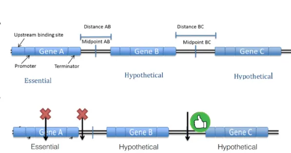
Figure 2: Figure 2A is a pictorial representation of a small genomic region as seen by our algorithm. Figure 2B shows the type of site we want to pick. We ideally want to pick sites that are midpoints between genes and are maximally far away from any gene. We also want to pick regions which are not close to any essential genes. Lastly we want to pick regions that are specific in the entire genome.

These metrics were chosen because irrespective of whichever factor we are trying to predict and optimize, ideally we do not want any of our integration sites inside any transcriptional region (genes along with their promoters). If we integrate a foreign gene inside the host transcriptional region, we will end up disrupting the host genome. Therefore as a preventative measure, we want to pick midpoints between genes to minimize the affect on the host genome. Additionally, we predict that we only want to integrate a new gene next to genes which are not essential, hypothetical or cryptic in order to minimize affects on the host

genome.

Essential genes in comparison to non-essential genes are genes, which if disrupted, will kill the organism while hypothetical genes are genes that are not confirmed to be genes [18]. Therefore integrating next to a hypothetical gene might not be as bad as integrating next to an essential gene since there a chance that the hypothetical gene is not a gene. Additionally cryptic genes are phenotypically silent DNA sequences, not normally expressed during the life cycle of the organism and only activated by mutation or recombination [19]. Therefore disrupting a cryptic gene, or a non-essential gene might not have a huge adverse affect on the host organism in comparison to disrupting an essential gene.

Lastly, we want to ensure that when we are integrating a gene it only goes in to the site we want it to go in to, i.e., specific integration. Our initial hypothesis was that if the site that we pick in the genome for integration is similar to a lot of other regions in the genome, our integration gene would end up integrating in to all of those regions. Thus we need to pick sites that are highly specific in the genome, so that we can direct the gene to go in to only that site specifically.

Scoring the Integration Sites:

Developing the algorithm included thinking about all the potential factors that we should be on a lookout for while looking for an ideal integration site. We aim to eventually factor in all the factors for site scoring as mentioned in the section above. However computing the score for a site (which quantifies the “goodness” of an integration site) is not very trivial because we have no information about which factor should weigh more than the other. For example, although intuition might tell us that the factor “integration site is next to an essential gene” should weigh more than the factor “distance from a neighboring gene”, we do not have any background data that proves it. We anticipate that overtime we would have to tweak around the weights of the scoring function in order to be able to come up with the most ideal scoring function and thus a correlation between all these factors. Therefore the algorithm was modified to be built in a way that the weights for each factor could easily be tweaked. Our

plan is to eventually settle to an ideal weighting metric (find the unknowns in the formula) by performing several integrations and using the integration data as a training dataset.

𝑆𝑖𝑡𝑒  𝑆𝑐𝑜𝑟𝑒 = 𝒂𝐷 + 𝒃𝐻 + 𝒄𝐶 − 𝒅𝐸 − 𝒆𝐵 where      𝐷 = 𝑑𝑖𝑠𝑡𝑎𝑛𝑐𝑒  𝑓𝑟𝑜𝑚  𝑛𝑒𝑖𝑔ℎ𝑏𝑜𝑟𝑖𝑛𝑔  𝑔𝑒𝑛𝑒, 𝐻 =   1  𝑖𝑓  𝑛𝑒𝑖𝑔ℎ𝑏𝑜𝑟𝑖𝑛𝑔  𝑔𝑒𝑛𝑒  ℎ𝑦𝑝𝑜𝑡ℎ𝑒𝑡𝑖𝑐𝑎𝑙 0  𝑜𝑡ℎ𝑒𝑟𝑤𝑖𝑠𝑒 ,      𝐶 =   1  𝑖𝑓  𝑛𝑒𝑖𝑔ℎ𝑏𝑜𝑟𝑖𝑛𝑔  𝑔𝑒𝑛𝑒  𝑐𝑟𝑦𝑝𝑡𝑖𝑐 0  𝑜𝑡ℎ𝑒𝑟𝑤𝑖𝑠𝑒 ,      𝐸 =   1  𝑖𝑓  𝑛𝑒𝑖𝑔ℎ𝑏𝑜𝑟𝑖𝑛𝑔  𝑔𝑒𝑛𝑒  𝑒𝑠𝑠𝑒𝑛𝑡𝑖𝑎𝑙 0  𝑜𝑡ℎ𝑒𝑟𝑤𝑖𝑠𝑒 , 𝐵 = 𝐵𝐿𝐴𝑆𝑇  𝑠𝑐𝑜𝑟𝑒

For my master’s thesis project, I simply focused on whether we can predict the specificity of integration.

For our initial set of integrations we wanted to see if we could predict the specificity of integrations using its BLAST (Basic Local Alignment Tool) [20] score which essentially is a measure of how conserved/non-conserved the site is within the genome. Therefore in the beta version of the algorithm, which includes the specificity module, a = 1, b = 0, c = 0, d = 0, e =1.

In order to get to the final version of the algorithm that would be able to predict ideal sites, we would need to identify through experimentation what the true values of the variables a, b, c, d and e are.

7. Algorithm Development

The algorithm development work had been previously initiated as part of my superUROP project. The algorithm, in its alpha version, scores all possible integration sites in E. coli and outputs a list of sites ranging from the most ideal to the least ideal sites. It is built keeping the

five main metrics in mind, i.e. the ideal integration site should not be inside the genes of the host genome, the ideal integration site should be maximally far away from the host genes, it should not be next to an essential (highly important to the host organism) gene and the site should be at a highly specific region in the genome. The factors from above were built in to the algorithm and all the possible insertion sites were determined and then scored (based on the scoring function given). Note that the current version is activated to only score the sites based on the specificity feature in order to be able to optimize that feature first.

The algorithm was written in python using the features of biopython [21]. We used the MG1655 E. coli databases (Version 16.5, Updated November 6 2012) for genes, binding factors, promoters and transcription units from the Ecocyc open source database. The algorithm first takes in a complete database which has information about all the genes, promoters, binding regions and transcription units. It then parses through the information to store instances of each transcriptional unit. The instances of transcription units, genes, promoters, binding regions are initialized as follows:

1) Gene

The constructor of a gene consists of its Unique ID (UID), gene name, left most position of the gene, right most position of the gene, essentiality boolean, cryptic boolean, hypothetical Boolean & direction of the gene (+ or -).

2) Terminator

The constructor of a terminator consists of its UID, it’s left most base pair position and its right most base pair position.

3) Promoter

The constructor of a promoter consists of its UID, its name, its transcription start site (plus1) and an upstream base pair value (default value currently set to 100 bp)

4) Bind Site

The constructor of a bind site consists of its UID, the length of the binding site (whose default value is set to 15 bp), and center (whose default value is set to None)

The constructor of a transunit consists of its UID, its name, and the position of its left most base pair, the position of its right most base pair and a set of components (genes) that are essential, cryptic, or hypothetical.

Once all the transcriptional units are identified the algorithm finds the midpoints between the transcriptional units. It then performs the scoring for all the midpoints based on the type of genes next to it and the BLAST score of 50 base pair homology arms of each site. The BLAST (Basic Local Alignment Search Tool) is an open source software from NCBI that takes in DNA sequence and a reference genome and produces a score that tells you how similar or dissimilar the DNA sequence is to the reference genome. Thus using BLAST on the 50 base pair homology arms gave us the information about whether the site was specific to the region or not.

The flowchart below breaks down the development of the algorithm in to series of steps:

Databases    

Obtain  the  Correct  databases  and  relevant  information  to  de?ine  the   relevant  components  (genes,  terminators,  trascription  units  etc)  

Parsers  

De?ine  parsers  and  parse  the  information  from  the  databases  

Intialization  

Use  the  Parsed  information  to  create  a  gene,   terminator,  binding  site,  transcription  unit  etc  

Scoring  

Find  midpoints  between  the  transcription  units   and  score  the  midpoints  

Results  

8. Developing the Specificity Module of the Algorithm

Picking Specificity as a Metric:

We picked specificity as an initial feature to optimize and predict. In order to understand whether our predictive approach would work, we performed preliminary experiments to see if we could predict the specificity characteristic of an ideal integration site (Factor D: When a construct is integrated at a site, it is integrated specifically in that site and not in other regions of the genome). We used the BLAST (Basic Local Alignment Tool) score of the homology arms of the score, which is essentially a measure of how conserved/non-conserved the site is within the genome. We expected to see that sites with a larger BLAST score (the site appears to be similar to other sites in the genome) has less specific integrations versus sites with a smaller BLAST score (the site is not similar to other regions in the genome) have more specific integrations.

Conducting Experiments to Predict Specificity:

For each site, its associated BLAST score was calculated by summing the score of the top 10 hits if there were more than 10 hits, or the sum of all the hits if there were less than 10 hits. Fifteen sites, with the highest BLAST score and the lowest BLAST score were selected and integrations were performed at those sites.

In order to perform lambda Red integration, homology arms of 50bp from each site (a site is a midpoint between genes), were picked and a construct with a KAN resistance gene was flanked. The resulting construct had the homology arms and gene for KAN resistance.

Each of the constructs was integrated in an E. coli strain (EcBZ14), prepared for lamba red recombination (MutS-) [Protocol: Appendix 1]. The resulting colonies were picked and using simple PCR procedures, the colonies were checked for specific versus non-specific integration.

A primer internal to the construct, and another in the genomic region were used to check if the construct had gone in specifically. This method however was not perfect since, if we did not see a PCR product, we were not able to figure out whether the construct had gone in non-specifically, or whether the PCR did not work due to experimental conditions. Secondly, we also wanted to analyze whether the colonies were mutations and where exactly did the construct end up integrating.

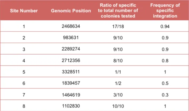
Although not a perfect method, we were still able to get some preliminary data regarding the specificity of some sites as shown in Table 1.

Table 1: The table shows each of the sites and their associated blast scores and percentage specificities. The data for the bottom three sites (highlighted) were obtained from a postdoctoral fellow in the lab (Bijan Zakeri).

Figure 3: A pictorial representation of how we checked our colonies for specific or non-specific integration. The forward primer bound to the construct with the KanR gene while the reverse primer flanked the genomic region. A positive PCR result showed specific integration.

Analyzing the Specificity Data:

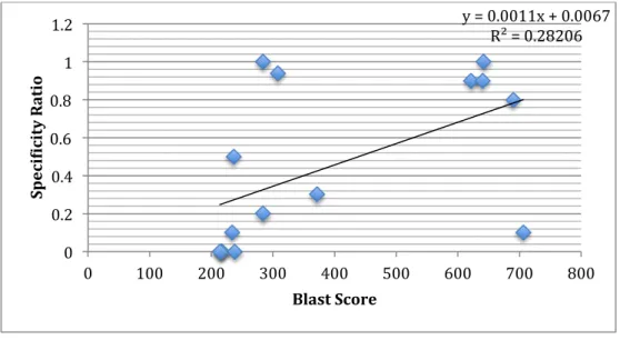
The specificity data we found for the sites was spread out enough for us to do some initial analysis including some high specificity and low specificity sites. We compared the BLAST scores for each of the sites with its specificity score (as mentioned, our hypothesis was that as the BLAST score of a site increases, its specificity should decrease since there are more regions available for homologous recombination). The following graph shows the results of the comparison.

The graph shows that the correlation between specificity and BLAST score was poor. We also examined whether we could find any other existing correlations between the specificity of integration at a particular site and the characteristics of that site for example correlation between GC content of the homology arms and specificity of integration, or the correlation between the predicted stability of DNA secondary structures that could occur in the ssDNA form of the homology arms and the specificity of integration.

y  =  0.0011x  +  0.0067   R²  =  0.28206   0   0.2   0.4   0.6   0.8   1   1.2   0   100   200   300   400   500   600   700   800   Spec i;ic ity  R atio   Blast  Score  

Figure 4: Graph representing the correlation between the BLAST score for sites and their specificity ratio. The correlation between the two was not strong enough to make a definitive statement.

We also analyzed the correlation between specificity and combination of the above-mentioned factors. The graphs in Figure 7 show the results.

y = -0.0206x + 0.0204 R² = 0.22407 0   0.2   0.4   0.6   0.8   1   1.2   -­‐40   -­‐35   -­‐30   -­‐25   -­‐20   -­‐15   -­‐10   -­‐5   0   Spec i;ic ity  

Free  energy  (Kcal/Mole)  

Stability of DNA 2 Structure

y = 0.0217x - 0.4923 R² = 0.23304 0   0.2   0.4   0.6   0.8   1   1.2   0   10   20   30   40   50   60   70   Spec i;ic ity   %  GC  Content  

GC Content vs Specificity

Figure 5: Graph representing the correlation between the stability of the DNA secondary structure for sites and their specificity ratio. The correlation between the two was not strong enough to make a definitive statement.

Figure 6: Graph representing the correlation between GC content of the homology arms for sites and their specificity ratio. The correlation between the two was not strong enough to make a definitive statement.

In none of these analysis did we find a strong correlation, leading to the conclusion that in order to predict even characteristics like specificity we would need a more sophisticated approach for example machine-learning. This would require a large dataset of integrations and associated data. The data will be needed to uncover any correlations and to train our algorithm to be able to predict whether a site is specific or not. This conclusion led us to formulating our second approach to tackle this problem.

Identifying some “Safe Harbors”:

As mentioned previously, this project started off as a DARPA project to propose a few “safe harbors” for integration to them. Although we had not yet formulated a predictive metric to find genomic sites that are highly specific for integration during our experiments we found some highly specific sites (shows at least 30% specificity). In most of these cases we observed colony growth within the normal expected time, i.e. there was no adverse affect on

Figure 7: Graphs representing the correlation between a combination of factors (GC content, DNA structure stability, BLAST score) for sites and their specificity ratio.

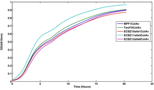
the growth of the organism. However, a few sites were picked and we performed growth rate experiments on them to determine any growth effects. The experiment was performed in a 96-well plate in a Tecan Infinite 200 Pro. Cells were first grown overnight to saturation (5ml LB in 15ml culture tubes), and then diluted down 100x into 200ul LB before loading onto the plate reader. Reads were performed every 1-minute, with 10seconds of 3mm amplitude orbital shaking prior to the reading. Figure 8 shows the growth curves of four different Safe Harbors. “MPF1colAv” is the non-integrated E. coli strain, while TwoFAColAv, EXBZ10site1colAv, ECBZ11site3colAv and ECBZ12site6colAv correspond to sites 1, 6, 7 and 8 respectively. As shown by the graph, we did not see any adverse effects on growth, whereas for site 7 we saw a slight advantage to grown due to the integration at that site.

Table 2: The table shows the sites we identified as “specific” based on specificity ratio 0.3 and above.

9. Limitations of Initial Approach

Once these safe harbor sites were identified, they were recommended to DARPA. However, previous analysis suggested that the data from 15 sites was not enough to reveal underlying trends -- unless the correlations are very strong, they will require many more data points to uncover. However, using the current protocol to integrate in to 150 sites was not possible either since each integration was very laborious.

Lastly, as mentioned previously, our method of identifying whether a site was specific or not (using simple PCR procedures) was not very robust. Our simple PCR approach was only useful to identify specific integrations but gave us no information about whether the PCR worked, or whether the construct went in to the genome non-specifically. In order to truly uncover the underlying correlations we needed to 1) integrate in to a lot more sites 2) be able to do it efficiently 3) and accurately identify where our construct got integrated.

In light of this need to generate a lot more data, we completely revised our experimental plan. We designed an approach for simultaneously performing 150 integrations and measuring the

Figure 8: The figure shows the growth curves of four different Safe Harbors. “MPF1colAv” is the non-integrated E. coli strain, while TwoFAColAv, EXBZ10site1colAv, ECBZ11site3colAv and

ECBZ12site6colAv correspond to sites 1, 6, 7 and 8 respectively (See chart on the left). All of the sites did

not show any adverse affects on growth rate of the organism due to integration.

0 5 10 15 20 25 0 0.1 0.2 0.3 0.4 0.5 0.6 0.7 0.8 0.9 1 Time (Hours) OD(A610nm) MPF1ColAv TwoFAColAv ECBZ10site1ColAv ECBZ11site3ColAv ECBZ12site6ColAv

specificity of the integrations using Next-Generation Sequencing (NGS). We believed that this dataset would allow us to search a wide range of genomic features to uncover correlations. Our revised plan to conduct large-scale integrations was as follows:

1) Pick 150 sites and build constructs to integrate (with KanR)

2) Performed pooled integrations of all the constructs simultaneously in to cells. 3) Selection in Liquid for KanR – increase the number of integrants

4) Sequence the entire population.

5) For each site, count the number of specific and non-specific integrations 6) Use the specificity data to identify correlations.

Section III

This section talks about our modified approach to tackling the problem. We conducted large scaled pooled integrations (at ~150 sites throughout the E. coli genome) and used Next Generation Sequencing to analyze the integration data. In this section we discuss the methods used to perform the experiments and the different approaches we used, how we analyzed the sequencing data and how we evaluated the integrity of the dataset. We also present the specificity data for all the integration sites and evaluate the correlations between the specificity data and characteristics we think might affect specificity. Lastly, we analyzed REP sites and whether integrating at those sites affect specificity or efficiency of integrations.

10. Modified Approach: Large-scale Pooled Integrations

In order to uncover the underlying trends between specificity and factors affecting specificity, we decided conduct large-scale pooled integrations and use NGS to analyze the specificity and non-specificity of the sites. The tasks that were therefore laid out were as follows:

1) Design a construct to integrate that would not only enable us to select on the integrants, but also allow us to distinguish between individual integration events.

2) Pick random 150 sites to integrate in. 3) Conduct the pooled integration experiment

4) Compare and contrast the integration results between the experimental, individual approach of integration versus the pooled and computation approach of integration to make sure that the different methods did not affect the specificity results.

6) Sequence the data from the experiments and analyze the data computationally.

Designing the Constructs:

Due to the large-scale pool approach to integrations, we had to ensure our constructs were designed in a way such that we would be would be able to identify separate integration events. Additionally since different integrations would give different growth rate affects, we wanted to have an identifier to be able distinguish between each instance of an integration once. This was made possible by making a construct with a Kanamycin resistance marker, flanked by 14 random nucleotides (which functioned as a marker to reduce bias and act as integration event identifier) and the corresponding 50 bp homology arms for each site as shown in Figure 9.

Figure 9: A pictorial representation of the construct used for the integration experiments. Along with the homology arms, the constructs contain a unique N14 barcode, and a KanR gene for selection.

Making Constructs:

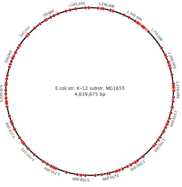
150 random integration sites were picked to integrate the constructs at. The sites were picked in a way to maximize the number of sites not in any transcriptional units. Table 3 shows all the sites (in bp) that were picked for the experiment.

Figure 10: The E. coli genome with all the integration sites we picked marked in red. Sites were picked throughout the genome for integration. Note that this is an approximation since the strain we used for the experiment is E. coli strain EcNR2 (mutS– , λ-Red+ ).

For each of these sites, the primers were ordered and the constructs were built using PCR [Protocol in Appendix].

Integration Experiment – Two Different Approaches:

Once the 150 constructs were made, they were integrated in to cells. The integrants were then pooled together in LB and the cells were allowed to recover. Once the cells had reached the saturation point in their growth phase, we performed genome extraction (1×10! _{cells) on the}

cells. This DNA was then sequenced to get the data.

3129289 2561255 696581 3859285 266112 2536599 3634073 2411317 720171 3193023 983631 2785404 1864659 1577531 4457435 4294138 1636965 1570286 931426 1647519 507941 1650826 1228602 3004004 302953 5606 2403632 2594863 1565366 2355944 3010525 819886 3049068 4116296 3760102 1952519 4534345 4091016 2689540 3638706 2566257 479248 3788277 249487 1416474 4106677 1211656 310934 4368537 3748977 2116586 3058750 2985294 642664 2627578 376647 1067142 189609 2980395 1291660 216079 4498499 2454116 4538412 892736 2509419 2196383 4158957 1639006 2414988 2314949 3181590 89294 1314298 167333 353942 1582161 1184931 640601 3861774 3267832 2209086 19715 502629 4460989 2000008 3055106 4499869 4539718 2010569 2234643 1292543 59483 1588223 2506393 2915951 1627130 4240477 1934507 3465117 3250131 2765449 4597630 4248717 4324973 4455259 578295 2405054 1653288 707280 4482403 1676200 271954 3161640 1608866 1179642 3376813 4530087 3134575 2641073 3502881 1096420 3080796 3779119 2541736 4312293 2513565 781059 3510531 3421330 3734278 695576 2224466 1937180 1464619 1529700 2039236 2723982 3825398 3623619

Table 3: The list of the ~150 sites we chose to integrate at for the experiment.

One of the uncertainties while integrating was the amount of time the cells needed to recover in the pooled integration before selection, such that we can minimize the growth rate bias of the different integrants and allow for integrated cells with low growth rates to grow as well. To allow for this we performed the experiment in two ways, altering the selection process each time.

Integration Experiment 1:

In the first integration experiment (protocol: Appendix 2), The constructs were integrated in cells (5 constructs integrated in one go, 200ng of each construct), when the cells were at 0.6 OD. The integrants were all pooled together in 200ml of LB and the cells recovered for an

Figure 11: The protocol used for the pooled integration experiment number 1. In this protocol, the cells were allowed to recover for one hour in 200ml of LB after which they were selected in Kanamycin.

hour. After an hour, 50ug/ml Kanamycin was added to the culture to select for the cells that had undergone integration. The genome was then extracted and used for sequencing. This protocol was the most similar to the integration protocol we had used earlier. However, it was unclear whether one hour of recovery time was enough for the more disruptive integrants to grow. Since this was an important piece of information to have, we decided to alter the selection step in experiment 2.

Integration Experiment 2:

In the second integration experiment (protocol: Appendix 3), The constructs were integrated in cells (5 constructs integrated in one go, 200ng of each construct), when the cells were at 0.6 OD. The integrants were all pooled together and allowed to recover overnight. The next day, the culture was diluted 1:100 in 2.8 L of LB-Kan (50ug/ml) to select for cells that had undergone integration. The culture was allowed to grow over night and genome extraction was done the next day.

Figure 12: The protocol used for the pooled integration experiment number 2. In this protocol, the cells were allowed to recover overnight and diluted 1:100 the next day in LB-Kan. The cells were given a lot more time to recover before selection.

Control Integrations:

For each experiment, in order to ensure that the integrations had occurred successfully, we also had positive (constructs we knew show some integration) and negative controls (no DNA, uninduced cells). The positive and negative controls were separated at the pooling step, allowed to recover individually and then plated on Kanamycin plates. For the negative controls we did not expect any colonies to appear on the plate, whereas for positive controls we expected to see a lot of the colonies.

Positive Control:

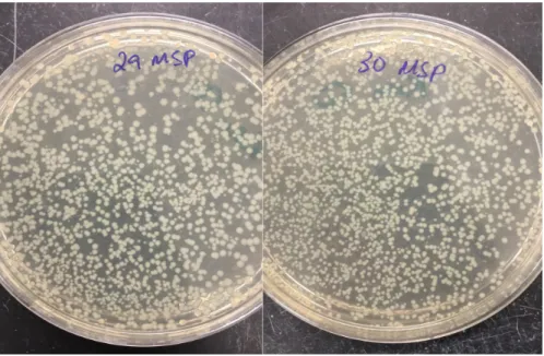
Two positive control samples were integrated to ensure that the cells were viable, the integration was successful and that integrating 5 DNA constructs together did not affect the integration event itself. Once integrated, the positive control samples were recovered in 1ml of LB. The cultures were then plated on Kan 50mg/ml plates. Both the plates show several colonies indicating that the integrations were successful.

Plate 29: Integration of sample 1 (containing DNA construct 1,2,3,4,5) Plate 30: Integration of sample 2 (containing DNA construct 6,7,8,9,10)

Negative Controls:

Plate 31: uninduced cells + DNA from sample 1 (Constructs 1,2,3,4,5) Plate 32: induced cells + no DNA (only water).

The negative control mixtures were electroporated and recovered overnight in 1ml of LB. The cultures were then plated on 50mg/ml KAN plates and the colonies observed.

Both the plates had little to no growth, allowing us to confirm that the integrations occurred successfully and that most of the cells that would grow in our actual experimental culture would be real integration events.

Cross Validation – Initial Approach versus New Approach:

One of the critical things was to ensure that the data we get from our new method of identifying the specificity of a site (pooled integrations, computationally analyzing sequences) is predictive of the data from the standard, traditional approach of integration (individual integrations, colony PCRs), otherwise the correlations we find would not be representative of the true wet-lab conditions.

Figure 14: The results of the negative controls done along with the pooled integration experiments. Sample 31 and 32 both contain 5 constructs each, validating that the integration experiment worked and that pooling technique is viable. We see no colonies on plate 32 and only some growth mutants on plate 31.

In order to be able to do this, we also built constructs for five other sites that we knew from prior experiments would be informative sites to integrate at (2468634, 1464619, 1102830, 983631, 2712356) in the same way as we built them for the rest of the 150 sites.

In the old method, the integrated cells are re-suspended in LB and recovered overnight. After which they are plated on Kan plates, which selects the cells that have undergone integration. Colony PCR is then performed on these colonies to identify whether the integration was specific or non-specific.

Figure 15: The differences between the old, standard approach of lambda Red integrations, in comparison to our new method of integrations and determining specificity. Instead of selecting cells on Kan plates, the integrants are selected in LB-Kan and genomes sequenced.

We however, revised the PCR approach (in comparison to the earlier experiments) to give us more information about whether our construct have integrated or not, and if integrated, had it gone in specifically. In order to identify this, the primers are designed in a way that the PCR might produce two products (Figure 16).

• If PCR with primer 1 and 3 is successful, we know that the construct integrated and integrated specifically.

• If PCR with primer 1 and 3 does not work and PCR with primer 1 and 2 is a small band, we can claim that the construct went in non-specifically or the colony was resistant because of a mutation.

• If PCR with primer 1 and 3 does not work and PCR with primer 1 and 2 is a big band, we can claim that the construct has probably gone in correct and that the PCR with primer 1 and 3 was just a false negative.

On the other hand, in the new method, the integrated cells are re-suspended in LB and recovered overnight. The cells are then diluted in LB-Kan and allowed to grow (selection step). The cultures then undergo genome extraction and the genomes are sequenced to reveal all the integration events. The specificity and non-specificity of integrations is determined using computational tools.

Figure 16: The modified approach to determining specificity using PCRs. Instead of just one reverse primer in the cassette, we used another reverse primer in the genomic region. If both the PCRs worked, we know the integration was specific but, if only PCR with primer 1 and 2 worked, it can tell us about whether we have a false negative PCR 1 and 3, or whether the construct went in non-specifically.

We performed this comparison for five sites. The constructs were integrated in to cells. Before the selection step, the integrant samples (1ml each) were split in to two samples (500ul each). One of the 500ul was selected in culture with Kanamycin, and the genome extracted and sequences. The other 500ul was plated on Kanamycin plates, the colonies counted and then analyzed (using the PCR method mentioned above) for specificity. The specificity results from both the approaches were very similar allowing us to conclude that the new approach and the old approach and comparable (The results are further explained in Section 13).

11. Enrichment of Relevant Sequences using Arbitrary PCR

Capturing the Data:

Before we sequenced the genome, we wanted to make sure that the amount of the data that we would get back from sequencing captures all the integration events that we expected to see to give us valid data.

Based on our previous integration experiments, we observed an average of 50 colonies per plate for each integration (each corresponding to a unique integration event). Given that we were integrating 150 constructs, we were expecting about 7500 unique integration events.

Since the Next-Generation Sequencing captures 1ng of DNA, we wanted to ensure that 1ng of E. coli genomic DNA would be able to capture 7,500 unique integration events.

Given that the E. coli genome is 5,000,000 bp long [22], and 1 mole of bp is 650g [23], 1 E. coli genome (5,000,000 bp) would be 5×10!!"  _{g. Since the sequencer captured 1ng of DNA,}

that would 1×10!! _{/ 5×10}!!" _{= 2×10}! _{(200,000) genomes, which is a lot more than 7500}

genomes. Therefore, we were confident, that using the sequencing method we would be able to capture all the integration events that occurred.

Preparing the Samples:

Now that we had the genomes from experiment 1, experiment 2 and the controls experiments, we needed to sequence the genomes. In order to do that we had to conduct a series of steps to successfully get the required data.

We had 7 samples:

1. Genome from Experiment 1 (Pooled Integrations) 2. Genome from Experiment 2 (Pooled Integrations)

3 – 7: Genome from control experiments (to check whether the computational and experimental methods give the same specificity results).

The first step was to shear the samples to our required size of 300-400bp so that we can cover the homology arm, the N14 barcode sequences, and enough genome to indicate specific or non-specific integration. We chose this size for sonication because the maximum read length of the MiSeq system for Illumina Sequencing is 300bp. The samples were sheared via sonication and the samples of size 250-400bp were selected for sequencing. An example of the genomic DNA sample (from experiment 2) after sonication, which was then run on the Advanced analytical Fragment Analyzer (by Advanced Analytical) to quantify the lengths of the sequences, is shown in Figure 17.

Figure 17: The results of the fragment analyzer run on one of the sheared sample. The average sheared size was ~400, which covers our 50 bp homology arm, N14 sequence and enough genomic region to know whether the integration was specific or not.

The next step (performed by the MIT MicroBio Center) was then to enrich for the parts of the genome that were relevant to us for sequencing (instead of sequencing the entire genome). An enrichment primer in our cassette that we used to build the constructs was used to enrich for the relevant sequences.

However, the enrichment was not successful in the first step due to the relative number of the relevant sequences being very small in comparison to the sequences from the entire genome. In order to troubleshoot for this, we used Arbitrary PCR (ARB PCR) techniques to enrich for the required regions, before sending the samples off for the sequencing enrichment step.

Enrichment Using Arbitrary PCR:

Arbitrary PCR [24,25,26] requires specific primers in the construct to bind to, and an arbitrary primer that will bind somewhere in the genome. We wanted to design the primers in such a way that we maximize the amount of genomic region that was captured in the sequencing, in order to analyze where in the genome the integration occurred.

The specific primer for the first round was designed to be 112 bp away from the N14 barcode sequence, and the specific primer for the second round was designed to be 66 bp away from the N14 barcode sequence.

Since we wanted at least 20 bp of the genomic region in order to understand whether the integration was specific or not, with high confidence, we wanted our product size after the first round of PCR to be at least 216 bp, or after the second round at least 170 bp.

We tried several different altered protocols of the Arbitrary PCR, mainly allowing for more cycles and time in the annealing round, or more cycles in the amplification round. The results we saw with more cycles in the amplification round were slightly better and so we used those moving forward [Protocol in Appendix].

In order to predict what we might see on the gel, we ran a simulation that picks a random N sequence from the sheared sample distribution, and enriches it using our primers.

Figure 19 is the resulting distribution of the length of the sequences. Note that for the simulation we estimated that our initial sheared distribution is a normal distribution with mean 405 and standard deviation 110 (which makes it an underestimating distribution, causing out simulation data to also be slightly underestimated; the higher bins should be a little larger and lower bins should we a little smaller.)

Figure 18: The internal specific primer is 112bp away from N14 and external specific primer is 66bp away from the N14. Round 1 of the PCR uses primer 1 and an arbitrary primer, and Round 2 uses primer 2 and a specific primer that bind to the tail of the arbitrary primers from round 1. All final arbitrary PCR products that are at least 170bp would give us at least 20 base pair of information regarding the genomic region the construct went in to.

Since there are many more ways a smaller sequence can be amplified in comparison to a larger sequence we amplify, we would have a lot more smaller sequences in our arbitrary PCR results, in comparison to large. However, as long we have a good population of sequences over 170 bp, we would be able to capture most of the integration events.

We therefore went ahead with the Arbitrary PCR approach in order to enrich the sample with the sequences that are relevant to us for sequencing (and the other parts of the genome are not amplified). Figure 20 shows the results of the arbitrary PCR (1: Enriched genome from Experiment 1, 2: Enriched genome from Experiment 2, 3: Enriched genomes of the positive control samples). The resulting genomes from the arbitrary PCRs were then given for sequencing.

Figure 19: A simulation of what length sequences we should expect from our Arbitrary PCR results. The simulation picks N random sequences from our sheared distribution population and enriches them using our arbitrary primers.

Lastly, we also wanted to validate that even though our arbitrary PCRs had worked, whether we able to achieve the purpose of the arbitrary PCR (only amplify genomic regions which had our constructs)

To this effect, we used the Arbitrary PCR products to test whether they contained regions that we were sure would have integrated (based on previous experiments). Therefore using a primer internal to the construct, and a genomic primer we tested for three sites we thought would have integrated and hence should show a positive result on the gel. We were able to successfully amplify those regions, indicating that our enrichment via Arbitrary PCRs was successful.

Figure 20: The final products of the arbitrary PCR (1: Enriched genome from Experiment 1, 2: Enriched genome from Experiment 2, 3: Enriched genomes of the positive control samples). This sample was used for Illumina Sequencing.

Figure 21 shows the results of the experiment conducted to check whether Aribitrary PCRs were able to enrich the required regions. Three different sites (1, 2 and 3) were tested on all three samples (A – experiment 1, B – experiment 2, C – positive controls). From the results we can see that all three of the regions show up to be positive, sites 1 and 2 seem to be specific, whereas for site 3, it seems like there was some non-specific integration. We further confirmed these results by sequencing the bands, and upon checking the sequences, we were able to confirm that these were true sequences that represented actual integration events. Sites 1 and 2 showed specific integration, whereas site 3 had non-specific integrations, hence the multiple bands.

Therefore we were able to move forward with sequencing the Aribitrary PCR products, enriched for our integration sequences confidently.

Figure 21: Results of the experiment conducted to check whether the ARB PCRs were able to enrich the required regions. Three sites were picked, and using primers in the construct and the genomic region, their presence was checked in the experiment 1, experiment 2 and positive control samples. The 2-log ladder was used for this experiment.

12. DNA Sequencing

Number of Reads:

The genomes were Illumina sequenced (MiSeq data) and the sequences were analyzed. We obtained ~2.5 Million reads. These reads were only 12.5% of the total data (as opposed to the usual 90% pass filter rate). Preliminary analysis showed that 75% of the first 9 nucleotides were C’s which resulted in a poor pass filter rate.

We suspect that the C bias is most likely in the N14 barcode sequence, which was prepared by Integrated DNA Technologies. The primers, because they were not hand mixed, probably carried forward some bias.

The priority, therefore, was to determine whether the data set could be used for analysis. We calculated the number of integrations observed per site, along with the number of unique integrations (as determined by the barcodes) per site. Many sites (60%) showed several integration events in addition to several unique integration events. Since the presence of this data would allow us to do a specificity count, we concluded that the dataset can be used for analysis, despite the low filter rate or 12.5%.

Figure 22: Histogram of the number of unique integrations (barcode counts) for each site. We see a large distribution in the number of unique integration events. Since the number of unique integration events determines specificity, we observe sites with both high and low efficiencies.

Figure 23: Zoom in of Figure 22 for Barcode counts between 0 and 50. There are several sites that have only a few integration events, i.e. have a low efficiency.

Our next step was to figure out whether the data coverage was high enough, i.e., whether we were able to obtain data for every site, given our sequencing data. Out of the 144 sites that we ended up integrating in, about 60% of the sites had integration events. The rest of the 40% that did not have any integration events most likely did not have any integration events not because of a lack of data, but because these sites were inefficient. This is further suggested by the data integrity analysis using our positive control sites. Figure 25 shows all the sites that were successfully integrated at (red) and all the sites that did not undergo successful integration (green).

Figure 24: Histogram of the percentage of unique barcode counts for each site. There was a large variation in the data (from 20% unique integrations to 90% unique integrations). Several sites had a large percentage unique barcodes i.e. unique integration events.

For the sites, that did have integrations, we observed a diverse number of integrations. Some sites (perhaps high efficiency sites) had hundreds of integrations, whereas some low efficiency sites (perhaps the integration had significant affects on the growth rate of the cells) had a smaller number of integrations.

Figure 25: The E. coli genome with all the integration sites that had successful integrations in red (sites on the outside of the circle) and the sites that did not have any integrations in green (sites on the circle). About 60% of the sites had at least one integration and 40% of the sites did not show any integration.

Figure 26: Histogram of the number of integrations/efficiency per site. Several sites had a large number of integrations.

Figure 27: Histogram of the number of integrations per site for sites that have less than 50 integrations.

Using all this data, we had to analyze whether our data set was complete (consists of enough observations to draw conclusions) and therefore whether the results that we concluded from the data set were meaningful.

As mentioned earlier, for 150 constructs we expected about 50 integration events on average each (from prior data), and therefore 7500 genomes. Based on our data set, out of the 7000 observed integrations, only 2000 of them were unique integration events, indicating that the average multiplication rate for an integrant was 7000/2000 = 3.5. Therefore for each of the 7500 predicted unique integration events, we could expect 3.5X times the sequences – 26.5 thousand sequences (1% of our dataset).

In order to examine whether this 1% is significant, we could do a statistical test. However, this is not of utmost importance since the ultimate test of whether our data is coherent is whether the predictions it makes are significant.

13. Analyzing the Integrity of the Data

In order to analyze the integrity of the dataset, we needed to calculate the specificity of all the sites.

Specificity of Sites:

The dataset was used to calculate the specificity of all sites. This was done computationally and the script was written in python using biopython and the BLAST modules.

For each of the sites, we checked for all the sequences in our dataset that contained its homology arm. Once we had all the sequences with the homology arm for a particular site, we got the associated N14 sequence, and the rest of the sequence that was the part of the genome site the integration occurred at. Using the BLAST tool, we then analyzed the genome sites, and marked an integration event specific if the genomic region was the same as what we had expected it to be had it gone in specifically, otherwise it was marked non-specific. Since this was done using BLAST, we accepted sequences with greater than 90% identity as specific.

Lastly, all the specific sequence counts were normalized by the number of unique barcodes that were seen. For example, if for a particular site we had seen the barcode before, we did not double count it in our specificity calculation.

Using this we were able to calculate the percentage specificity for all the sites that had at least one integration (spreadsheet in Appendix). The specificity data had a large spread; we had some sites that were completely non-specific, and some that were highly specific (>90% specificity). Specificity % of sites >90% 26 >80% 35 >70% 42 >60% 44 >50% 48 >40% 53 >30% 57 >20% 61 <10% 32

for each site in our list of sites:

store all the sequences in the dataset in which its homology arm exists for each of those sequences containing the homology arm:

identify the barcode sequence identify the genomic region

check if the genomic region is what we expected --> mark it specific/non-specific

use the barcode sequences to normalize for integration events return the percentage specificity for each of the sites

Figure 28: Pseudo-code for how we computationally calculated the specificity of all the sites.

Figure 29: The graph shows the histogram of sites and their % specificity. We observed a large spread in specificities – many sites were highly specific, or not specific at all. About 42% of the sites had greater than 70% specificity whereas 32% of the sites had less than 10% specificity.

26% of the sites had specificity of greater than 90%, 42% of the sites had specificity of greater than 70% (highly specific sites) and about 32% of the sites had specificity of less than 10% (highly non-specific sites).

We then further wanted to analyze the characteristics of some of the sites that showed no integration, or one’s that showed highly specific integration.

Sites Without Integration:

These sites were analyzed using the EcoCyc Database [27]. Most of the sites that showed no integration were either inside a pseudogene (Functionless relatives of genes that have lost their gene expression in the cell or their ability to code protein) [28], next to a gene for conserved protein, or inside a gene (although we tried to pick midpoints as sites, some of the sites were still inside a gene because either the homology arm overlapped with the gene, or there were newly annotated genes which were not present in Version 16.5 of Ecocyc Database that we used for computational purposes). A few examples of such sites are as follows:

1) Site 2032688, showed no integration, in a pseudogene Yed_S2.

This gene is interrupted, meaning it is a fragment of a larger coding sequence with an inserted stop codon. (No Literature Information)

2) Site 4460989, showed no integration, inside a gene treC, trehalose-6-phosphate hydrolase (enzyme)

Figure 30: A pictorial representation of the possible role of Yed_S2 in E. coli. [Figure from EcoCyc database]

3) Site 2925855, showed no integration. Next to a conserved protein ygdH, function unknown.

Highly Specific Sites:

Some high specific sites were analyzed using the EcoCyc online database. Many sites that were observed did not have another gene in the next 200bp of site, or were in a specific type of extragenic sites called Repetitive Extragenic Palindrome (REP) Sequences (Table 5).Some examples of highly specific sites are as follows:

1) Site 781059

No gene in the surrounding 200bp of the site. Specificity: 97.6

Number of Integrations: 182

2) Site 2314949

In extragenic site, REP162d Specificity: 89.4

Number of sequences: 22

Figure 31: A pictorial representation of the possible role of treC in E. coli. [Figure from EcoCyc database]

Figure 32: A pictorial representation of the possible role of ygdH in E. coli. [Figure from EcoCyc database]