DOE/ET/51013-130
ANTENA USER GUIDE
Brian McVey Plasma Fusion Center
Massachusetts Institute of Technology Cambridge, MA 02139
July 1984
This work was supported by the U.S. Department of Energy Contract No. DE-AC02-78ET51013. Reproduction, translation, publication, use and disposal,
in whole or in part by or for the United States government is permitted. PFC/RR-84-13
Abstract
Use of the computer code "ANTENA" is described. The code calculates the vacuum fields and the linear self-consistent plasma fields for a variety of ICRF antenna configurations.
Contents
1. Introduction 3
2. Availability and Execution 8
3. Input 10
4. Output 17
5. Compilation 19
Appendix A. Subroutine Input and Input Files 23
3
1. INTRODUCTION
The computer code "ANTENA" calculates the vacuum fields and the linear self-consistent plasma fields for the ICRF antennas of Fig. 1.1. In addition, the computer code has an array capability whereby any combination of the antennas contained in Fig. 1.1 may be superimposed (Fig. 1.lh is an example). Along with the electric and magnetic fields, the radial power deposition profiles, the radial power flow, and the antenna impedance
(including mutual impedance between coils) is computed. The antenna-plasma geometry is diagrammed in Fig. 1.2. An antenna is located between the plasma boundary at r - a and an outer conducting wall at r - c. The inside radius of the antenna is at r - b. The antenna current is assumed to be uniform over the length of the antenna. The plasma parameters and the magnetic field are assumed to be functions of radius with the magnetic field oriented in the z-direction. The M.I.T. Report #PFC/RR-84-12, "ICRF Antenna Coupling Theory for a Cylindrically Stratified Plasma", contains detailed
information on the physics assumed in the computer code "ANTENA".I
The field quantities are calculated by numerically performing the inverse transformation;
ik z+in# F(r,o,z) -dk
2
zz
ir
F(r,n,k) zFig. 1.1 Various
ICRF
Antennas
a.
full
turn loop
pama
( B
vacuk
b. saddle coil
c.
Nagoya
type
M
e. line current
f. partial turn loop
h. array
4 half
.
half Nagoya
turn loops
angular
rture
.rect
ape
I
'00
5
Fig. 1.2
Antenno
-
Plasma Geometry
C
b
a
=
plasma radius
b
=
inside
radius of coil
F(rnkZ) J(n,k ,b,c) (2) D(n,kz,n ,B 0T)
where J represents the excitation level of a (n,k z) mode by the antenna, and D contains the plasma response to the imposed fields.
Figure 1.3 diagrams the basic structure of the computer code "ANTENA". Through a namelist, INPUT reads all the parameters that are required to define the problem diagrammed in Fig. 1.2. The following subroutine,
INITLZE performs various calculations such as conversion from cm. to m., sets up radial plasma profiles, etc. The plot and print subroutines write the input information to disk files. Now we are at the main loop in the program. IVAR is the independent variabl,e for which the fields are calculated. Examination of Eqs. (1) and (2) suggest IVAR can take on many different values; r, 0, z, W/£ i, f, n e, T, T , Bo, kz, and other user defined variables. Dependent upon the value of ISPECTR, either the integrand of Eq. (1) is calculated by SPECTRM or the inverse transformation is performed by INTEG. The subroutine INTEG either performs a Fourier sum
2
or uses the integrator package DRIVE . Each of these subroutines calls FIELDS which calculates Eq. (2) for a given n, kz mode. Finally, the computed field quantities are written to disk files, and the process is repeated for a new value of IVAR. Figure 1.3 is a general flow chart of
"ANTENA". More detail may be obtained by reading the listing of the main program.
7
FIG. 1.3 FLOW CHART FOR ANTENA
vSTART INPUT INITLZE PRINT PLOT IVAR =IVARLOW > IVARHI
STOP IVAR PLINT
<IVARHI
ISPE CTR SPECTRM
0
2. AVAILABILITY AND EXECUTION
The program is available from directory,
1437 .ICRF
The directory contains the source program, ANTENA4 and executable programs
XANTENA4, for the A-machine; and XANTENC4, for the C-machine. The program is executed by the statement,
XANTENA4 I - IN 0 - OUT P - PLOT / t v
where IN is an input file that contains three namelist inputs, OUT is a text output file, and PLOT is a text file that contains data for subsequent plotting. The default files are I = terminal, 0 = terminal, and P -plotout.
A separate plotting program (PLOTA4) processes the file designated by P. Plotted output may be obtained by executing XPLOTA4 on the A-machine or XPLOTC4 on the C-machine. The execute line is,
XPLOTA4 I = IN? 0 = OUTP P = PLOT / t v
where P = Plot is the disk file generated by ANTENA, INP is a namelist input file that contains control parameters, and OUTP is an output file that is a
9
directory of the frames plotted. The default files are I - terminal, 0
-terminal, P - plotout.
The codes are subscripted by the number 4 indicating a version number. Number 4 is the most recent version number and previous versions have been moved to directory .ICRFOLD . The file ANTNEWS will contain information on the status of the code. It presently contains a list of changes made in version 4 of the code compared to earlier versions. It also contains a directory of the codes in .ICRF .
3. INPUT
Communication to ANTENA is through three namelist inputs contained in the subroutine INPUT. A listing of the INPUT subroutine is included as Appendix A. In that subroutine, the DATA statements define the default values of the input variables. The first namelist contains control,
scanning and integration parameters.
NAMELIST INPUT1 Selected output may
to zero or one. ICOORD = 0 S1 IBFLD = 1 = 0 IEFLD - 1 - 0 IPABS 1 - 0 IEDOTJ =
1
=0be controlled by setting the following parameters equal
rectangular coordinates cylindrical coordiantes
the magnetic field calculation is on the magnetic field is not calculated the electric field calculation is on the electric field is not calculated the power absorption calculation is on the power absorption is not calculated the antenna impedance calculation is on the antenna impedance is not calculated INDVAR determines the independent variable for the inner loop.
INDVAR - 1 2 3 4 5 6 7 r scan # scan z scan w/w (1) scan c frequency scan density scan IB0 1scan
T(j) scan where J = IPART 8
11
k scan
z
user defined scan through subroutine INDVAR1O
The range and increment of the independent variable are defined by, starting value
end value
incrementing step
The variables INDVAR2, IVARLOW2, IVARHI2, IVARINC2 have the same meaning as above and provide control over an outer independent variable scan. The outer scan is de-activated by defining INDVAR2 to be less than zero. The fields that are computed by the code are determined by the following parameters. ISPECTR -
0
- 1
IFIELD -1
-2 INTEGKZ - 2 -3 =4 IFAST -1
=0
ISLOW - 1=0
use integration routines
calculates the Fourier spectrum inductive vacuuim fields
plasma fields
variable step integrator Fourier sum, Ez (± L/2) - 0 Fourier sum, E(z) - E(z+L) fast mode fields are calculated fast mode fields are not calculated slow mode fields are calculated slow mode fields are not calculated
1
For the meaning of IFAST and ISLOW refer to the physics description.
The parameters used by the drive integrator (INTEGKZ - 2) are the following.
KMINCM minimum value of k in cm
z
-1
KMEAXCMt maximum value of k in CM
z
KSTEPCM initial step size for k in cm
EPS
error bound for the integrator
9
10
IVARLOW IVARHI IVARINC I IThe default values for the integration parameters provide reasonable accuracy (refer to reference 2).
NAXIAL defines the number of k modes summed for z
INTEGKZ - 3,4
NMAX the n summation of Eq. (1) extends from ±NMAX
NAMELIST INPUT2
The second namelist contains the dimensions for the plasma, for the antenna, and defines the nominal position and wave parameters.
ACM the plasma radius in cm
CCM the vacuum chamber radius in cm
LENGCM axial length used in Fourier sums (INTEGKZ 3,4)
The following coordinates define the position at which the fields are calculated.
RHOCM radial position in cm
PHIDEG azimuthal position in deg
ZCM axial position in cm
The nominal wave parameters are the following.
WNOR w/w (1) where 1 is the first plasma species C
defined.
FREQ used to define w when FREQ > 0
KZOCM axial wave number that is assumed in spectral scans (ISPECTR - 1)
NAZIM aximuthal mode number that is assumed in spectral scans. The default value is NAZIM
--99. If NAZIM is set to be larger than -30, only n - NAZIM is calculated in the Fourier sums and integration for ISPECTR = 0.
13
The antenna parameters are,
is the number of coils in an array is an integer array
individual coils in (i.e. ICOIL - 1 3
that determines the the array
5 7) The following coils are modelled,
ICOIL -
1
-2 -3 -4-5
-6 -7full turn loop saddle coil
Nagoya type III coil rectangular aperture line current
partial turn loop half Nagoya coil
The following parameters define the interconnection of coils in an array. ISERIES > 0
IPARALL > 0 IMUTUAL - J
IANTCON -1,2,3,or 4
NSTEP
the coils are connected in series the coils are connected in parallel
the "J" th coil is driven with current and the mutual impedance between that coil and
others is calculated.
designates that the coil interconnection is defined in a user supplied subroutine
ANTCON1, etc.
defines the number of radial points in the E J integration for the impedance
r r
calculation of coils with radial feeders
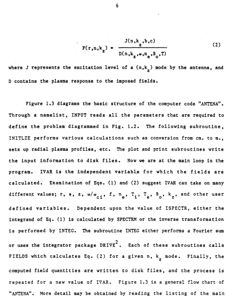
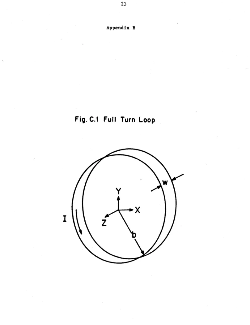
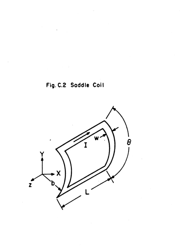
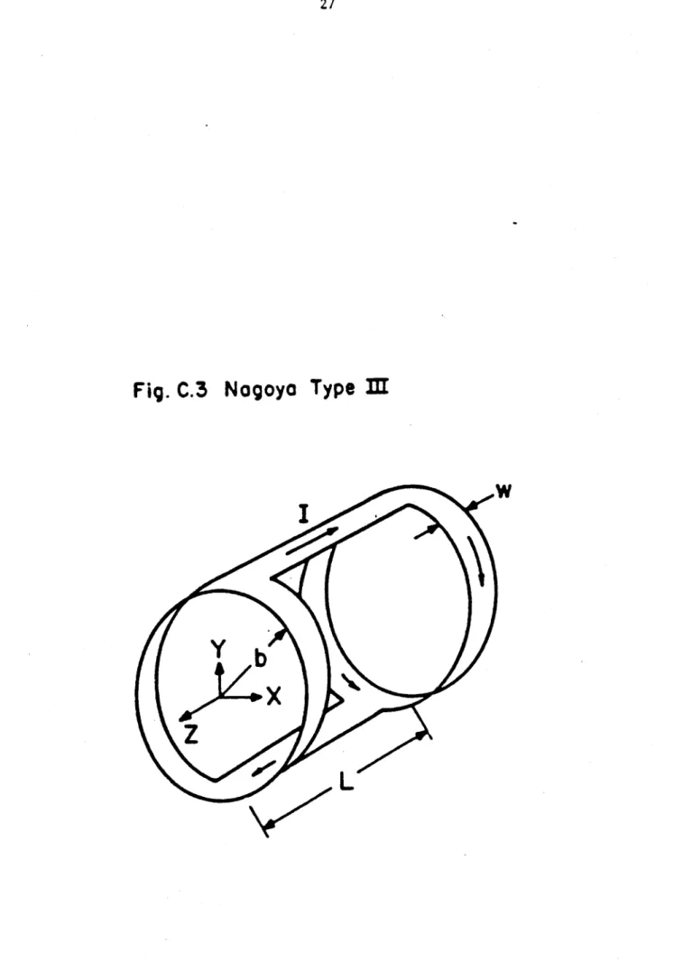
The antenna dimensions and the orientation of the antennas are defined by the following arrays. Appendix B contains detailed drawings of the various antenna configurations.
is a complex number that defines the current in each coil. For ICOIL - 4, CUR defines the magnetic field over the rectangular aperture.
is the inner radius of the coil.
NCOILS
ICOIL
CUR
--- I
LNGCM is the characteristic length of the coil. ANGDEG is the angular extent of the coil.
ZOCM is the axial location of the coil. PHIODEG is the azimuthal location of the coil. The default location is at the origin.
NAMELIST INPUT3
The final namelist defines the plasma parameters and the radial profile. IKIJ is an integer flag that determines the plasma
response. IKIJ - 1 is a Maxwellian velocity distribution.
NPART is the number of plasma species. BFLD vacuum magnetic field in Gauss. NTOT plasma density in particles/cm .
The following are all real arrays defining the parameters of the various plasma constituents.
MASS in atomic mass units
CHARGE units of electrons charge
CONC concentration in %
TPAR parallel temperature in eV
TPER perpendicular temperature in eV
COLFREQ effective collision frequency using a Krook
The following profiles.
IPROF
model
parameters determine the stratified density and temperature
= 1 -2 -3 =4 uniform profile parabolic profile Gaussian profile
15
NSTRAT the number of strata < N3
WDENCM density scale length
WTEMPCM an array defining the temperature scale length for each species
The magnetic field in the plasma is calculated from B (r) - BFLD /1 -(r) For profiles, the parameters TPAR and NTOT are the r - 0 values.
Experimental profiles are defined by the following input arrays.
RS defines the positions of the interfaces
between strata.
FDEN defines the density profile.
FTEMP defines the temperature profiles.
FDEN and FTEMP is normalized to the first element in the array where the density at r - 0 is NFLD * FDEN(1) and the temperature at r - 0 is TRAR(1) * FTEMP(1,1) and TPAR(2) * FTEMP(2,1).
Communication to PLOTA4 is through a single namelist.
ILABLE is a lable flag that when larger than zero will write the words contained in the array lable on each plot.
LABLE is an array of up to 5 words that contains a message.
XLABLE when INDVAR - 10, a 3 word user supplied
message contained in XLABLE will be printed on the x-axis of the graphs.
IPARAM - 1 orders the sequence of plotting so that all (B , etc.) graphs appear adjacent to one another.
Sample input files for ANTENA and PLOT4A are contained at the end of Appendix A.
17
4. OUTPUT
The output generated by ANTENA consists of two text files. The first file designated by 0 - _ _ _ _ on the execute line, is a formatted file that tabulates the field calculation. The second file designated by P
-on the execute line is read by PLOTA4 and generates graphical output. The description in this section, assumes the reader has run ANTENA4 and PLOTA4, for the default parameters and has generated the text and plot output files.
The first 120 lines of the text file mirrors the input namelist. The fields are then tabulated as a function of the independent variable. The field format is either in rectangular or cylindrical coordinates dependent upon the value of ICOORD. For each field component, the modulus and phase
-1
is plotted. The phase is in degrees, and the modulus is in volts Cm for the electric field and in units of Gauss for the magnetic field. The local power absorption "PABST" is the total power absorbed in a infinitely long cylindrical shell of radius r and of cross sectional area equal to one
square cm. Integrating over the cross section, 2w
4
PABST rdr yields the total power absorbed by the plasma. The output "PABSI" indicates the power absorption by the various species, I - 1,NS where each species was definedin the namelist input. The output "POWER" is the total power absorbed inside a cylinder of radius r (i.e. the power flow across the surface of a cylinder of radius r). Finally the source impedance is calculated for each coil. The complex power flow out of the coil is calculated, and then the resistance and reactance is computed.
namelists. Frames 8 - 11 plot the plasma profiles that have been assumed.
In the field plots, the* solid curve refers to the modulus on the left-handscale and the dotted curve refers to the phase on the right-hand scale. The same convention is used on the source impedance plots.
For spectral scans (ISPECTR - 1) the output units are all multiplied by one centimeter. In addition, the plasma radial wave numbers are plotted.
19
5. COMPILATION
To enlarge the memory, to use options INDVAR - 10, IANTCON 4 0, or to
change the source code; it is necessary to recompile ANTENA. The memory storage of ANTENA is determined by the following parameters which may be found in the CLICHE ANTCOM4.
Ni - 9 is the maximum number of coils in an array. N2 - 3 is the maximum number of plasma species. N3 - 50 is the maximum number of strata in a profile. N4 - 21 is the maximum number of spatial positions for
the inner scan at which the fields are calculated.
For compilation on the A or C machines, the .parameter KMACH must be set as indicated in ANTCOM4.
The "ANTENA" code uses the integration package contained the source 2
code INTPROG4 . This program is dimensioned to accommodate up to NEQU - 400 first order differential equations. The parameter NEQU must be set to a value larger than N7 in ANTCOM4. INTPROG4 has been compiled and libraries LINTGA4 (A-machine) and LINTGC4 (C-machine) may be found in directory 1437 .ICRF . Libraries may be constructed by using LIBMAK on the A-machine and BUILD on the C-machine.
file, say LIBI and then recompiling an executable code with the following lines.
A-machine
CHATR P - ANTENA4 LIB - (F', LINTGA4, LIB1)
/
t vC-machine
PRECOMP ANTENA4 PANTEN
/
t vCFT I - PATAN / t v
LDR X - XANTENC4, LIB = (FORTLIB, LINTGC4, LIBI) / t v
Two examples are offered to illustrate the use of INDVAR = 10 and IANTCON
-1. The following subroutine defines the separation distance between two antennas as the independent variable.
1 SUBROUTINE INDVARIO(NOPT) 2 USE ANTCOM4
3
4 C THE INDEPENDENT VARIABLE IS LABELLED. 5
6 DATA LABLE1(10)/" ZB(CM) "/
7
8 C Zt(2) IS THE AXIAL POSITION OF COIL NUMBER TWO. 9 18 IF (NOPT) 11,12,13 11 12 C Z8(2) IS SAVED. 13 14 11 SAVE(1)-Z3(2) 15 RETURN 16 17 C Z0(2) IS INCREMENTED. 18 19 12 ZB(2)=IVAR*.Z1 20 RETURN 21 22 C ZB(2) IS RESET. 23 24 13 Z8(2)=SAVE(I) 25 RETURN 26 27 END
Results from the use of this subroutine are contained in reference 1 in Fig. 7.4 .
21
The following subroutine provides the interconnection required in the calculation of the source impedance for the array illustrated in Fig. 1.lh.
1 SUBROUTINE ANTCON1 2 USE ANTCOM4
3
4 C PSOURCE(I) IS THE COMPLEX POWER FLOW OUT OF ANTENNA "I". 5 6 Cln2.*PSOURCE(1)/CABS(CUR(1))**2 7 C2a2.*PSOURCE(2)/CA8S(CUR(2))**2 8 C3'2.*PSOURCE(3)/CABS(CUR(3))**2 9 C4s2.*PSOURCE(4)/CABS(CUR(4)f**2 10
11 C DEFINE THE SERIES - PARALLEL CONNECTION.
12 C C1,C2,...C8 ARE COMPLEX CONSTANTS THAT MAY BE USED. 13
14 CIuC1+C2
15 C3-C3+C4
16 C1*C1*C3/(Cl+C3) 17
18 C DEFINE RESISTANCE AND REACTANCE AND TOTAL POWER FLOW. 19 20 RANTEN(1)mREAL(CI) 21 XANTEN(1)*AIMAG(CI) 22 PSOURCE(I)uPSOURCE(1)+PSOURCE(Z)+PSOURCE(3)+PSOURCE(4) 23 24 RETURN 25 END
When the above (found in 1437
subroutines are compiled to build LIB1, the file ANTCOM4
.ICRF) must be in your local directory.
The memory N1 -N2 -N3 -N4 -N5 -N6 -allocation of PLOTA4 5 is the maximum 3 is the maximum 50 is the maximum 102 is the maximum 31 is the maximum 16 is the maximum
is defined by the following parameters, number of coils in any array.
number of plasma species. number of strata in a profile. of 2 * N3 + 2 or N5
number of points in an inner scan. number of points in an outer scan.
References
1. B. D. McVey, "ICRF Antenna Coupling Theory for a Cylindrically
Stratified Plasma", PFC/RR-84-13, Massachusetts Institute of Technology (1984).
2. A. D. Hindmarsh, "GEAR. . Ordinary Differential Equation System Solver", UCID-30001 Rev. 3 Lawrence Livermore Laboratory (1974).
Appendix A
I C -- - - - -f - -ff-m- - - - - -f - - --
-2 C SURROUTINE INPUT: THE INPUT DATA FILE IS READ 3 C THROUGH THREE NAMELISTS.
4
s SUBROUTINE INPUT 6 USE ANTCOM4
7
a C FIRST NAMELIST: 1) OUTPUT CONTROL PARAMETERS.
9 C 2) INNER AND OUTER SCAN PARAMETERS. 3) FIELD PARAMETERS. 11 C 4) INTEGRATION PARAMETERS, 5) MISCELLANEOUS.
11 12 NAMELIST /INPUT1/ 13 1 ICOORD.IBFLD.IEFLD.IPASS.IEDOTJ. 14 2 INOVAR.IVARLOW.IVARJIIVARINC.IPART. 15 . INDVAR2.IVARLOV2.IVARNI2.IVARINCZ. 16 3 ISPECTR.IFIELD.INTEGKZ.IFAST.ISLOW. 17 4 KMINCM.KMAXCM,KSTEPCM.EPS.MF. 18 . NAXIAL.NMAX. 19 S ISIMEO 25 21 DATA 22 1 INDVAR//.IVARLOJ/I./.IVARHI/15./.IVARINC/3./.IPART/1/. 23 , INDVAR2/-1/.IVARLOW2/5./.IVARMI2/1./.IVARIMCZ/2./. 24 2 ICOORD/B/. BFLD/1/.IEFLD/I/.IPABS/1/.IEDOT/1 /. 2S 3 ISPECTR/5/.IFIELD/2/.INTEGKZ/2/.IFAST/1/.ISL-w/1/. 26 4 KMINCM/1.E-5,.KMAXCM/1.E1/.KSTEPCM/1.E-7/.EPS/1.E-4/.MF/13/. 27 * NAXIAL/105/.NMAX/S/. 28 5 ISIMEO/1/ 29
35 C SECOND NAMELIST: 1) PLASMA AND MACHINE DIMENSIONS.
31 C 2) NOMINAL POSITION AND WAVE PARAMETERS, 3) ANTENNA PARAMETERS.
32 C 4) ANTENNA CURRENT. DIMENSIONS. AND POSITION. 5) MISCELLANEOUS.
33 34 NAMELIST /INPUT2/ 35 1 ACM.CCM.LENGCM. 36 2 RHOCM.PHIDEG.ZCM. 37 . WNOR.FREO.KZOCM.NAZIM. 38 3 NCOILS.ICOIL. 39 . ISERIES.IPARALL.IMUTUAL.IANTCONNSTEP. 45 4 CUR.8CM.WIDCM.LNGCM.ANGDEG. 41 . ZBCM.PHIZDEG. 42 5 VOLTS.INDUC 43 44 DATA 45 1 ACM/1S./.CCM/3S./.LNGCM/55B./. 46 2 RNOCM/5./.PHIDEG/./.ZCM/S./. 47 . WNOR/./.FREO/-3.E6/.KZOCM/.01/.NAZIM/-99/. 48 3 NCOILS/1/.ICOIL/6/. 49 . ISERIES/f/.IPARALL//.IMUTUAL/B/.IANTCON/S/.NSTEP/3/. 55 4 CUR/(155g..5.)/.CM/20./.WIDCM/1I./.LNGCM/0./.ANGDEG/180./. SI . Z3CM/5./,PHI8DEG/5./. sz S VOLTS/-1./.INDUC/1./ 53
54 C THIRD NAMELIST: 1) PLASMA PARAMETERS. 55 C 2) RADIAL PROFILE PARAMETERS.
56 57 NAMELIST /INPUT3/ sa I IKIJ.NPART.SFLD.NTOT. 59 . MASS.CHARGECONC.TPAR.TPER.COLFREO. 65 2 IPROF.NSTRAT, 61 . WDENCM.WTEMPCM.W8FLDCM. 62 , RS.FDENFTEMP.FBFLD 63 64 DATA 65 1 !KIJ/1/.NPART/2/.BFLD/2.E3/.NTOT/2.E12/. 56 . MASS/I.,5.447E-4/.CMARGE/1..-I./.CONC/1lI..155./, 67 . TPAR/1. .105./,TPER/100.,1I./,COLFREO/2-1.E3/. 68 2 IPROF/2/,NSTRAT/1/. 69 . WOENCM/15./.WTEMPCM/2Z..25./ 78 71 READ (5.INPUTI) 72 READ (S.INPUT2) 73 READ (SIMPUT3) 74 75 RETURN
Sample Input Files
Default input file,
I S 2 9
3 S
The following example illustrates the use of multiple scans and inputs on experimental plasma profile:
1 INDVARw6 IVARLOWo1.E11 IVARHI-1.5E12 IVARINC-2.E11
2 INDVARZ4 IVAELOW2..7 IVARH12-1.1 IVARINC2-.05 3 IFIELDa2
4 IEFLDUf IIFLDbs IPABSOO
5 2 6 ACH816. CCM.25. 7 IHOCM=16. ZCMS25. PHI5DEG-95. 8 WNORa1. 9 ICOILw4 15 BCMo25. WIOCNm14. LNGCM=4B. 11 CUAe(45..5.) 12 S
13 NTOTw4.E11 TPAR045I. 32. COLFREQO1.E4 1.ES 14 TPERe2.E3 35. 15 SFLD=1.5625E3 16 IPROFu4 NSTRAT=5 17 RS11. 16.26 16.6 15.75 16. is FOEMaI. .7 .4 .1 .53 19 FTEMP. 1. 1. N. 25 1. 1.5. 21 1. 1. 5. 22 1. 1.5. 23 1. 1.5. 24 s
Appendix B
Fig. C.1 Full Turn Loop
Y
zx
Fig. C.2 Soddle Coil
27
Fig. C.3 Nogoya Type
I
Yb
Fig. C.4o Rectongulor Aperture
y
40--Br
29