A
PPLICATION OF THEP
ROBABILISTICC
OLLOCATIONM
ETHOD FOR ANU
NCERTAINTYA
NALYSIS OF AS
IMPLEO
CEANM
ODELMort Webster, Menner A. Tatang, and Gregory J. McRae
ABSTRACT
This paper presents the probabilistic collocation method as a computationally efficient method for performing uncertainty analysis on large complex models such as those used in global climate change research. The collocation method is explained, and then the results of its application to a box model of ocean thermohaline circulation are presented. A comparison of the results of the collocation method with a traditional Monte Carlo simulation show that the collocation method gives a better approximation for the probability density function of the model’s response with less than 20 model runs as compared with a Monte Carlo simulation of 5000 model runs.
1. INTRODUCTION
In the study of global climate change, an understanding of the various atmospheric, oceanographic, economic, and ecological processes relies heavily on the use of computer models. As scientists try to capture more detail and complexity of these processes, the models become more complex and more computationally expensive to run.
At the same time, our understanding of all of these aspects is highly uncertain, and this uncertainty is reflected in the models. Quantifying and characterizing the effects of these uncertainties is crucial to informing the policy process. Unfortunately, most traditional methods of uncertainty analysis of models are infeasible when applied to complex models of
climate change.
The probabilistic collocation method (Tatang, 1994) is a tool designed to enable uncertainty analysis of computationally expensive models at a very low computational cost. The general collocation method is one of several mathematical techniques for reducing a model to a simpler form (e.g., differential equations to algebraic equations). The probabilistic collocation described here adapts the general technique by using random variables to represent the uncertain
parameters. This paper will explain the basic concept of the probabilistic collocation method, and use its application to a model of ocean thermohaline circulation to show how the method works, when and how it can be used for uncertainty analysis, and to present a sample of the results it can yield.
Before describing how the probabilistic collocation method works, we briefly discuss the two main goals of an uncertainty analysis tool as applied to the task of studying climate models. First, it should take any model as a “black box” that has some set of inputs or parameters and some set of outputs or responses it produces. Second, it should use a description of the uncertainty in each parameter to be considered, usually in the form of a probability density function. Given the model and the uncertainty descriptions of the parameters, we would like the tool to give us:
• the probability density function of the response(s) of interest, • sensitivity analysis information,
• variance analysis information, and
A traditional method of obtaining probability density functions of responses from the
probability density functions of parameters is the Monte Carlo method. Essentially, this approach entails randomly selecting a value for each uncertain parameter from its uncertainty range, weighted by the probability, running the model for these values, and then repeating this process many times over. Then a histogram is made of the set of values of a response from the runs to obtain the probability density function. Because the values are selected at random, this usually requires many runs of the model, often on the order of thousands or more, to obtain reasonable results.
Traditional approaches to uncertainty analysis such as Monte Carlo, even with structured sampling and other techniques to improve its efficiency, are not feasible for application to complex climate change models. The computational time needed for just a single run of the model can be very large. One solution to this problem is to find a simple approximation of the model’s behavior with information gathered from only a small number of runs of the original model. This is the approach of the probabilistic collocation method.
2. COLLOCATION METHOD
2.1 The Underlying Concept
The basic concept of the probabilistic collocation method is to try to approximate the response of the model as some polynomial function of the uncertain parameters:
Ri = fi (P1, . . . , Pn). (1)
Once this simple approximation—essentially a reduced form model of the original model—is found, it can be used with all the traditional uncertainty analysis approaches, such as Monte Carlo, to extract the desired information. If some approximation with a very small margin of error can be found with a small number of model runs, we have solved the problem of performing uncertainty analysis on a complex model.
As an example, suppose we have some “black box” model:
Y = f (A, B) (2)
Our goal is to find an approximation: ˆ
Y = f´ (A, B) (3)
where f´ is a simple polynomial function of A and B which simulates the behavior of the model. For example, we might choose to represent ˆY as a function of first order or linear polynomials of A and B, H1(A) and H1(B) respectively:
ˆ
Y = Y0 + Y1H1(A) + Y2H1(B) (4)
Assuming that we already know H1(A) and H2(B), we only need to find the coefficients Y0,
Y1, and Y2 in order to solve for this approximation. By running the model three times to obtain three triplets (A, B, Y), we can solve for Y0, Y1, Y2 by substituting into Eq. (4).
The crucial step in efficiently estimating a good approximation is the choice of the values of the input parameters. In the above example, we want to choose three pairs (A, B) in a way that captures as much of the behavior of Y as possible. Since A and B are uncertain parameters with associated probability distributions, we want to choose the pairs of (A, B) to span the high probability regions of their distributions.
To do this, we borrow an idea from the Gaussian Quadrature technique of estimating integrals. In the Gaussian Quadrature method, we can estimate the integral of a polynomial as a summation with no error by using the roots of the next higher order polynomial. Similarly, in the probabilistic collocation method, we use the roots of the next higher order polynomial as the points at which to solve the approximation.
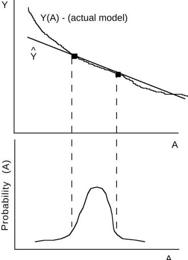
Assume, for example, that we are to derive polynomials of different orders based on the probability density function P(A). To estimate a linear approximation of Y = f (A) we need two points that span the high probability region of P(A). The roots of the second order polynomial
H2(A) provide these two points. Figure 1 illustrates this example. By using the two points bounding the high probability region of P(A), we can get a good estimation for ˆY . The larger
deviation of ˆY from Y only occurs in the low probability region and is thus contributes only a
small error.
A Y
A Y(A) - (actual model)
Probability (A)
Y^
So what we need then is a way to derive a set of polynomials from the probability density function of each input parameter such that the roots of each polynomial are spread out over the high probability region for the parameter. We can find these by deriving orthogonal polynomials. The definition of orthogonal polynomials is:
P x x ( ) ∫ Hi(x) Hj(x) dx = Ci ∂ij (5) where ∂ij = 1 if i = j = 0 otherwise
Hi(x) and Hj(x) are orthogonal polynomials of order i and j of x, and P(x) is some weighting function. In other words, the integral of the product of two orthogonal polynomials of different order is always 0.
For any probability density function P(x), we can derive the set of orthogonal polynomials for that distribution, by using P(x) as the weighting function. We always define the −1th order polynomial to be 0 and the 0th order polynomial to be 1:
H−1(x) = 0 (6a)
H0(x) = 1 (6b)
To find the first order orthogonal polynomial H1(x), we substitute into Eq. (5):
P x
x ( )
∫ H1(x) (1) dx = 0 (7)
By using the known probability density function P(x), we can solve for H1(x). Once H1(x) is known, it can be recursively used to find H2(x), and so on. In this way, we can find a set of orthogonal polynomials derived from the probability density function of the uncertain parameter. There are several actual techniques for analytically deriving orthogonal polynomials from a given weighting function (see, for example, Beckmann, 1973, and Gautschi, 1994).
It is important to remember that the orthogonal polynomials are derived solely from the probability distribution of the parameters, before ever running the model. These polynomials are used in two ways. Most importantly, they are used to generate the parameter values for
evaluating the model (which we refer to as the collocation points) and solving for the
approximation. We also use the orthogonal polynomials in the polynomial approximation of the model ˆY . We could actually use any form of polynomial for the approximation, but the
properties of the orthogonal polynomials make uncertainty analysis particularly efficient. For example, the expected value or mean of the approximation ˆY in Eq. (4) is simply the constant Y0. Similarly, the standard deviation and other statistical measures are simple to calculate by using the properties of orthogonality.
2.2 A Simple Illustration
To illustrate the collocation method, suppose the model to be analyzed has two parameters A and B, and one response variable Y:
However, we who are analyzing its uncertainty characteristics do not know the relationship between A, B, and Y: it is a black box. The steps in performing the uncertainty analysis are illustrated in the flow diagram in Figure 2. The analysis proceeds through these steps as follows.
Add higher order chaos expansion terms to polynomial
Check error of approximation
Yes
No
Use approximation for uncertainty analysis Run model on collocation point
and solve for approximation Specify uncertainty distribution
of paramters
Derive orthogonal polynomial for the distributions
Generate a polynomial chaos expansion of order to approximate model response
n
Generate collocation points for model runs
Is error too large?
Step 1: Specify uncertainty distributions of parameters
First we must specify the uncertainty in the parameters. Suppose that A has a uniform probability distribution from 1.0 to 10.0, and that B has a normal distribution with a mean of 2.0 and a standard deviation of 1.0.
Step 2: Derive orthogonal polynomials for the distributions
Next we must derive the set of orthogonal polynomials for each of these distributions. Starting with the variable A, we derive the polynomials as described above, substituting in P(A) and H0(A) = 1 into Eq. (5) and solving for H1(A). This process is then repeated for the higher order polynomials. The actual algorithm used for deriving the orthogonal polynomials is called ORTHPOL (Gautschi, 1994).
For A, the first five orthogonal polynomials for its distribution are:
H1(A) = A − 5.5 (9a)
H2(A) = A2 − 11A + 23.5 (9b)
H3(A) = A3− 16.5A2 + 78.6A − 99.55 (9c)
H4(A) = A4− 22A3 + 164.1429A2− 474.5714A + 425.1571 (9d)
H5(A) = A5− 27.5A4 + 280A3− 1292.5A2 + 2631.071A − 1826.393 (9e) Note that in order to simplify the calculations without any loss of generality, all orthogonal poly-nomials are generated in monic form, so the coefficient of the highest order term is always one.
While orthogonal polynomials are directly generated for uniform and most other distribution types, gaussian distributions are treated differently. Every normal distribution for random variable X can be represented by the transformation:
X = µ + σ(H1(ξ)) (10)
where µ is the mean of X, σ is the standard deviation of X, and H1(ξ) is the first order orthogonal polynomial of the standard normal distribution ξ, which has a mean value of 0 and a standard deviation of 1. This has the advantage that we can use the same set of orthogonal polynomials for any normal distribution, rather than deriving a distribution specific set for each normally
distributed parameter.
The orthogonal polynomials for the standard gaussian ξ are the Hermite polynomials:
H1(ξ) = ξ (11a)
H2(ξ) = ξ2− 1 (11b)
H3(ξ) = ξ3− 3ξ (11c)
H4(ξ) = ξ4− 6ξ2 + 3 (11d)
H5(ξ) = ξ5− 10ξ3 + 15ξ (11e)
From our earlier assumption that µB = 2 and σB = 1, parameter B is thus represented as:
Step 3: Generate polynomial chaos expansion1
Next we need a polynomial expression to represent the response variable as a function of the orthogonal polynomials of random variables A and ξ. This is called the polynomial chaos
expansion. Since the model is a black box, we might use a linear approximation as a first guess. The linear approximation is:
ˆ
Y = Y0 + Y1H1(A) + Y2H1(ξ) (13)
We can evaluate the model at different values of A and B (derived from ξ) to obtain Y. Since
H1(A) and H1(ξ) are known, we only have to solve for Y0, Y1, and Y2. To solve for these three unknowns, we need three triplets of (A, ξ, Y). Thus we need to run the model three times.
Step 4: Generate collocation points for model runs
In order to find a good approximation for the model with the fewest number of model runs, it is important to carefully select the parameter values, or collocation points. As noted earlier, the method for selecting collocation points is derived from the same idea as the Gaussian Quadrature method to numerically solve integrals. In the collocation method, we select the points for the model runs from the roots of the next higher order orthogonal polynomial for each uncertain parameter.
Since we are solving for a linear approximation, we use the second order orthogonal polynomials in choosing the collocation points. For A, the roots of H2(A), Eq. (9b), in order of increasing probability2 are (2.901924, 8.098076). For B, we use the second order polynomial H2(ξ), Eq. (11b), to find the roots: (−1, 1). Substituting into Eq. (12), the collocation point values for B are: (1, 3).
From these roots, we need to choose three pairs of points (Ai, Bi) to solve the model. The first pair will always be the highest probability root for each parameter. This is called the anchor point. The other points are selected by keeping one parameter at its highest probability value, and choosing the next lower probability root for the other. Thus the three input sets are:
(8.098076, 3) (8.098076, 1) (2.901924, 3)
Step 5: Solve approximation
We run the model for each of the three input sets, and save the corresponding response Yi. Then, substituting each triplet (Ai, ξi, Yi) into the approximation from Eq. (13), we can solve the three simultaneous equations for the three unknowns: Y0, Y1, Y2. For this example we get:
Y0 = 51
Y1 = 11
Y2 = 13
1The term “chaos” here is a technical term from the literature of numerical methods, and it has no relation to the
common notion of chaos in non-linear systems. The polynomial chaos expansion is simply the term for the polynomial approximation.
Using these values in Eq. (13), we get the reduced form model approximation.
Step 6: Check error of approximation
Before using the approximation, we need to check to see how good the approximation is. To check the error, we need to run the model a few more times, and compare the model results to the approximation results. For the error check model runs we need more collocation points. These points are derived from the next higher order orthogonal polynomials. We use the next higher order because if the errors are too large and we need a higher order of approximation, we will already have the model solutions we need to solve the approximation.
For the first-order approximation, we generate the error run collocation points from the third order orthogonal polynomials H3(A) and H3(ξ). The roots, in order of increasing probability are:
H3(A): (8.985685, 2.014315, 5.5)
H3(ξ): (1.732051, −1.732051, 0) and using Eq. (10),
B: (3.732051, 0.2679492, 2)
The collocation point input sets, starting with the anchor point, are: (5.5, 2)
(5.5, 0.2679492) (2.014315, 2) (5.5, 3.732051) (8.985685, 2)
For each of these input sets, we solve both the real model Y and the approximation ˆY . The error εi for each run is computed as:
εi = di 2
fAξ (•) (14)
where di = ˆY − Y, and fAξ (•) is the joint probability density function at the corresponding values of uncertain parameters. Then we measure the overall error as the sum-square-root (ssr) error:
ssr= ∑= εi ξ i fA 1 5 5 ( . , )5 5 0 (15)
or the relative sum-square-root (rssr) error:
rssr ssr E Y =
( ˆ) (16)
where E Y( ˆ) is the expected value of ˆY . Note that in computing the ssr, we use the joint
probability density function at the anchor point. Similarly, errors can also be computed relative to only one of the uncertain parameters rather than all of them jointly.
Since the ssr is dependent on the magnitudes for the typical values of Y, the normalized rssr is a more useful measure of the error. For this example, the ssr is 6.114 and the rssr is 0.120. Although the degree of accuracy required may be problem specific and determined by the modeler, the rssr of O(10−1) in this example is quite large and indicates that this is a poor
approximation.
Step 7: Try second order approximation
Since the error is large, we need to add higher order terms to try to obtain a better
approximation. As a next step, we might try adding second order terms, as well as a first order cross product term. The new polynomial chaos expansion is:
ˆ
Y = Y0 + Y1H1(A) + Y2H1(ξ) + Y3H2(A) + Y4H2(ξ) + Y5H1(A)H1(ξ) (17) To solve this new approximation, we must solve for the six unknowns (Y0, ..., Y5). Thus we need six sets of collocation points from the roots of the third order orthogonal polynomials. We have already found the roots and constructed five of the six input sets in the error checking step above. We need one more input set corresponding to the cross-product term. For this, we use the second-highest probability root for both A and B, (2.014315, 0.2679492). Running the model for this one point, and reusing the solutions from the error check, we can solve the coefficients for the approximation: Y0 = 51 Y1 = 11 Y2 = 15 Y3 = 1 Y4 = 6 Y5 = 0
Next we must check the error for this approximation. Since it is a second order
approximation, we use the roots of the fourth order orthogonal polynomials, and generate eight input sets as above. Running the model on these input sets and comparing with the
approximation results, we calculate the ssr as 1.784 and the rssr as 3.498 x 10⁻². This error is
still somewhat large. (The reader of this paper knows, as the hypothetical analysts do not since they see only a black box, that the actual model has a third order term for B, so the lack of a third order term in the approximation accounts for the error.) Also note that the coefficient of the cross-product term is 0, thus there is no cross interaction between A and B (which is a correct representation of the model).
Step 8: Try third order approximation
In an attempt to further reduce the error of the approximation, we can increase the order of approximation to third order:
ˆ
Y = Y0 + Y1H1(A) + Y2H1(ξ) + Y3H2(A) + Y4H2(ξ) +
Y5H3(A) + Y6H3(ξ) + Y7H1(A)H1(ξ) (18)
Using the model results from the fourth order collocation points used previously to check the error, we can solve for (Y0, ..., Y7):
Y0 = 51 Y1 = 11 Y2 = 15 Y3 = 1 Y4 = 6 Y5 = 0 Y6 = 1 Y7 = 0
To check the error, we must again solve for the roots of the fifth order orthogonal
polynomials, generate the collocation points, run the model ten more times, and calculate the error. This time the ssr error is 3.83 × 10⁻⁶ and the rssr is 7.50 × 10⁻⁸, which indicates an
extremely accurate approximation.
Step 8: Use approximation for uncertainty analysis
Now that we have found a sufficiently accurate approximation which is a simple polynomial, we can use this for a variety of statistical analyses. Although this is a simple example, if a large complex model can be reasonably approximated with a third order polynomial such as Eq. (18), performing a Monte Carlo simulation to obtain the probability density function of Y becomes feasible. Other information such as the mean or standard deviation are even simpler to obtain. For example, the mean of Y is the expected value E Y( ˆ), which is just the coefficient Y0 of the approximation. This is a result of the use of orthogonal polynomials; the expected value of every other term in ˆY is 0 because they contain products of different order orthogonal polynomials
(including H0(x) = 1). The standard deviation is similarly simple to calculate.
3. APPLICATION OF THE COLLOCATION METHOD TO AN OCEAN MODEL
To illustrate the process of using the probabilistic collocation method to perform uncertainty analysis, we will describe experiments performed on a box model of thermohaline circulation. The model is the simplest of three developed by Nakamura et al. (1994) in order to explore the mechanisms of destabilization of different thermohaline equilibrium states.
3.1 Model Description
The model geometry is a simplified coupled ocean-atmosphere model with two uniformly mixed boxes representing the atmosphere, and three boxes for the ocean (see Figure 3). The atmosphere spans one hemisphere, while the ocean is a 60˚ longitudinal sector from 10.44˚N to 75˚N representing one ocean basin based roughly on the North Atlantic. All boxes are separated at 35˚N, which is where observed zonal mean time-averaged net radiative forcing is zero and where the annual mean northward heat and moisture transports are near their peak. The ocean is a three box model based on (Stommel, 1961). Boxes 1 and 2 have the same surface area, so the volume of box 1 is equal to the sum of the volumes of boxes 2 and 3. Box 1 has a depth of 4000 m and box 2 has a depth of 400 m.
H H Low Latitude High Latitud Box 1 Box 2 Box 3 Te Te T S T S T S 2 2 2 2 1 1 Fw Fw 1 1 3 3
Figure 3. Three-box ocean model.
The temperature and salinity in each ocean box, denoted as Tn and Sn (n = 1, 2 ,3)
respectively, are uniformly mixed. The temperatures of boxes 1 and 2 represent the zonal mean surface temperatures at 55˚N and 20˚N, respectively. The volume flux that results from the thermohaline circulation between two adjacent ocean boxes, q, is represented as being proportional to the surface density flux, which is in turn a function of the temperature and salinity fluxes:
q = k [α(T2 − T1) − β(S2 − S1)] (19)
where k is a proportionality constant, and α and β are the thermal and haline expansion coefficients of seawater. A positive volume flux is assumed to be a flow from box 2 to box 1, box 1 to box 3, and box 3 to box 2, which is a high-latitude sinking state.
The density in boxes 1 and 2 are changed by exchange of heat and freshwater with the atmosphere, and by the advection of heat and salt. Box 3 only changes as a result of advection. Thus, the general equations for the time rates of changes of the temperatures and salinities in the ocean boxes are given by:
∂ ∂ T t H C M q T T V 1 1 w w1 m 1 1 = + ( − ) m = 2 for q > 0, m = 3 for q < 0 (20) ∂ ∂ T t H C M q T T V 2 w w m 2 = 2 + − 2 2 ( ) m = 3 for q > 0, m = 1 for q < 0 (21) ∂ ∂ T t q T T V m 3 3 3 = ( − ) m = 1 for q > 0, m = 2 for q < 0 (22)
∂ ∂ S t H V V q S S V 1 s 1 1 m 1 1 = − + ( − ) m = 2 for q > 0, m = 3 for q < 0 (23) ∂ ∂ S t H V V q S S V 2 s 1 2 m 2 = + ( − ) 2 m = 3 for q > 0, m = 1 for q < 0 (24) ∂ ∂ S t q S S V 3 m 3 3 = ( − ) m = 1 for q > 0, m = 2 for q < 0 (25)
where Cw is the specific heat of water, Hs is the virtual total salinity flux out of box 1, and Vn,
Mwn, and Hn are the volume, mass of water, and total surface heat flux for box n. The virtual total salinity flux Hs is derived from the total net freshwater flux into box 1, Fw, by:
H S F
M
s r w w1
= (26)
where Sr is the reference salinity, and Fw is in turn a function of the net of evaporation and precipitation (E – P).
The simplest model represents the atmosphere by mixed boundary conditions, in which sea surface temperatures (SST) are restored to a prescribed state, and the freshwater flux is fixed. As opposed to the more complex model in Nakamura et al. (1994), in which heat fluxes depend on the latitudinal temperature gradient and the radiative forcing, this model parameterizes the heat flux by the Newtonian Cooling Law:
H C M Te T 1 w w1 n n n = − τ (27)
where τn is the thermal relaxation time and Ten is the surface equilibrium temperature that would be attained if there were no oceanic heat transport. In this model, a further simplification is the specification of a fixed salinity flux Hs. The model performs an Euler integration of Eqs. (20)– (25) over a long time period (4000 years) to reach a stable equilibrium state from initial values. In models of thermohaline circulation such as this one, there exist multiple stable equilibria. For many parameter sets there exists both a high-latitude sinking equilibrium and a low-latitude sinking equilibrium. This model and its more complex versions were built to explore the stability of these equilibria, and the transitions between equilibria that result from perturbations
(Nakamura et al., 1994). For this purpose, the most complex model was tuned to find a stable high-latitude sinking state (among others), which simulates today’s climate. The volume flux for the North Atlantic ocean basin (ignoring transport from the Southern Ocean) is thought to be roughly 10 Sv (1 Sv = 106 m3s−1). The tuning used the proportionality constant k, which in these
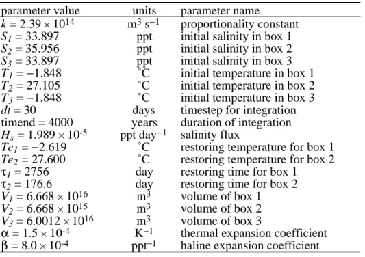
simple models represents the physics of the thermohaline circulation. Once a parameter set for a stable high-latitude sinking equilibrium was found, this was used to find appropriate values for the simpler model, including τn, Ten, and Hs. The resulting set of parameters for a stable high-latitude sinking equilibrium for this model is shown in Table 1. These values were used as the starting point in the following uncertainty analyses.
Table 1. Stable equilibrium parameter values for ocean model.
parameter value units parameter name
k = 2.39 × 10¹⁴ m3s−1 proportionality constant S1 = 33.897 ppt initial salinity in box 1
S2 = 35.956 ppt initial salinity in box 2
S3 = 33.897 ppt initial salinity in box 3
T1 = −1.848 ˚C initial temperature in box 1
T2 = 27.105 ˚C initial temperature in box 2
T3 = −1.848 ˚C initial temperature in box 3
dt = 30 days timestep for integration
timend = 4000 years duration of integration
Hs = 1.989 × 10⁻⁵ ppt day−1 salinity flux
Te1 = −2.619 ˚C restoring temperature for box 1
Te2 = 27.600 ˚C restoring temperature for box 2
τ1 = 2756 day restoring time for box 1
τ2 = 176.6 day restoring time for box 2
V1 = 6.668 × 10¹⁶ m3 volume of box 1
V2 = 6.668 × 10¹⁵ m3 volume of box 2
V3 = 6.0012 × 10¹⁶ m3 volume of box 3
α = 1.5 × 10⁻⁴ K−1 thermal expansion coefficient β = 8.0 × 10⁻⁴ ppt−1 haline expansion coefficient
3.2 Uncertainty Experiment
The first step of an uncertainty analysis of this model requires identifying the uncertain parameters we wish to study. For this analysis two parameters with the greatest uncertainty were identified. The proportionality constant k represents the physics of many of the oversimplified processes. In practice, it is tuned to a value that yields results consistent with empirical data, and thus the “correct” value is highly uncertain. Another parameter with great uncertainty is the salinity flux Hs. It is derived from the net of evaporation and precipitation of freshwater over the ocean and runoff from land, which are very uncertain and variable. For the response variable of interest, we selected the equilibrium volume flux q. Thus in this experiment we are interested in the effects of uncertainty in k and Hs on q.
Initial estimates were made of the probability distributions of k and Hs. For the specified parameter values, stable values for k would be in the range of 1 × 10¹⁴ to 4 × 10¹⁴m3s−1. A
uniform probability distribution between these values was used for k. The uncertainty in Hs is a function of the uncertainty in E – P, based on empirical measurements. An estimate of the uncertainty in E – P had a distribution from 0.55 to 1.15 m yr−1. This gives a β distribution3 of H
s from 1 × 10⁻⁵ to 3 × 10⁻⁵ ppt day−1, where the highest probability is at 2 × 10⁻⁵ ppt day−1.
However, there was a problem in applying the collocation method to this model with these parameter ranges. Because of non-linearities in the model, there is a bifurcation in the
equilibrium states. This bifurcation is shown in Figure 4. For all values of k and Hs above the
3 The original distribution of H
s was assumed to be uniform from 1 × 10⁻⁵ to 3 × 10⁻⁵. After reviewing the initial results, the model experts revised the distribution to be β, with the mean at 2 × 10⁻⁵ as shown in Figure 8. Because of the computational efficiency of the collocation method, iterative experiments can allow the experts to glean insights into the model and revise uncertainty estimates.
line, the equilibrium state may be either high-latitude sinking or low-latitude sinking, while below the line only low-latitude sinking is possible. For the other parameter values used (see Table 1), values of k and Hs above the line will result in a high-latitude sinking state.
Because the ocean model is small, we were able to apply the Monte Carlo method to find the resulting probability distribution of the volume flux resulting from the assumed uncertainty ranges of k and Hs. The results, in Figure 6, indicate the discontinuity between the low-latitude and high-latitude sinking solutions. The problem for the collocation method is in this
discontinuity. A key assumption of the collocation method is that the response surface can be approximated by a polynomial. A discontinuous surface is difficult if not impossible to approximate by a polynomial, and thus the collocation method fails to find a reasonable approximation with small errors. Figure 5 shows a scatterplot of the response surface of the volume flux as a function of k and Hs. This type of surface is impossible to approximate with a polynomial.
Figure 6 shows the resulting discontinuity in the probability distribution of the response, which is a product of the discontinuity in the response surface. Figure 7 compares a 9th order approximation by the collocation to the Monte Carlo results. Clearly the collocation method is unable to approximate the response accurately.
Although the collocation method does not work for the problem as initially formulated, the knowledge of the bifurcation can be used to redefine the problem in a way which allows the application of the collocation method. In this case, since we are interested in realistic solutions under today’s climate conditions, the low-latitude sinking states are not feasible solutions. Further, some investigation of the model yielded the almost linear correlation between k and Hs which locates the bifurcation. Using this relationship, we can redefine the uncertain parameters to ensure that we only examine ranges above the line in Figure 4.
0 0.5 1 1.5 2 2.5 3 3.5
Multiple Equilibria (realistic) Region
Unrealistic Solution Region
k
(High-Latitude Sinking)
(Low-Latitude Sinking)
0.994699 1.193638 1.392578 1.591518 1.790457 1.989397 2.188337 2.387277 2.586216 2.785156 2.984096 equilibria boundary ( , reference)
k – Hs Te
τ
H s
(5.0) 0.0 5.0 10.0 15.0 k 1.0 1.5 2.0 2.5 3.0 3.5 q
Figure 5. Response surface of volume flux.
0.00 0.10 0.20 0.30 0.40 Volume Flux (Sv) (5) 0 5 10 15 Probability
0.00 0.10 0.20 0.30 0.40 Volume Flux (Sv) Monte Carlo Collocation 9th order Probability (40) (20) 0 20 40 60
Figure 7. Collocation vs. Monte Carlo for fixed range of k.
We use a linear approximation of k as a function of Hs, since k is arbitrary relative to Hs, and
Hs has physical meaning. The uncertainty in k is then expressed as some ∆ above the line in Figure 4, thus remaining in the realistic solution space and avoiding the discontinuity. Thus k is defined as:
k = f (Hs) + ∆k (28)
The revised probability distributions for the two uncertain parameters are shown in Figure 8 and Figure 9.
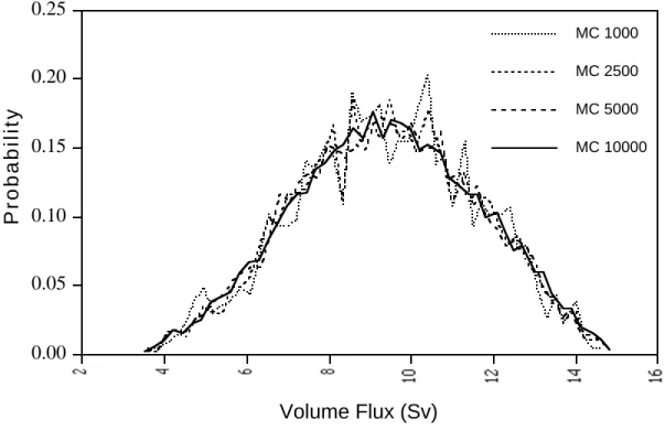
To provide a benchmark for comparing the results of the collocation method, we also
performed Monte Carlo simulations on the reformulated model.Figure 10 shows the results from the Monte Carlo for different numbers of model runs. Because Monte Carlo selects points at random, many runs are needed to obtain a reasonably smooth probability density function of the response. From Figure 10, it appears that at least 5000 runs are needed before the errors
associated with the random selection become small.
Using the Monte Carlo simulation with 10,000 runs as a benchmark, we compare the results of three approximations from the collocation method in Figure 11: linear, second-order, and second-order with a cross-product term. All of these are quite close approximations, with both second-order approximations being barely distinguishable from the Monte Carlo results.
The linear approximation required only eight runs of the model (three to solve plus five to check the error), while adding second-order terms required an additional seven runs, and adding a cross-product term requires two additional model runs. This is a significant savings in
computation time over the more than 5000 runs required for equivalent accuracy from the Monte Carlo technique.
0.00 1.00 2.00 ∆k 0.00 0.25 0.50 0.75 1.00 Probability
Figure 8. Probability density function for ∆k.
0.20 0.30 0.40 0.50 0.60 0.70 Probability 1.00 1.50 2.00 2.50 3.00
Salinity FluxH s (ppt/day 10 × –5 Figure 9. Probability density function for Hs.
0.00 0.05 0.10 0.15 0.20 0.25 Probability Volume Flux (Sv) MC 10000 MC 5000 MC 2500 MC 1000
Figure 10. Monte Carlo results for different numbers of runs.
0.00 0.05 0.10 0.15 0.20 Probability Volume Flux (Sv) MC 10,000 Coll - second-cross Coll - second order Coll - linear
Numerically, in terms of the relative sum-square-root error measurement, the error of each level of approximation is:
• linear: 9.23 × 10⁻³
• second-order: 5.16 × 10⁻³
• second-order with cross-product: 4.38 × 10⁻³
The collocation method allows the extraction of other information besides the probability density function of the response. The mean, standard deviation, and other moments can be easily calculated. Also, correlations between any two parameters, two responses, or a parameter and a response can be plotted over the uncertainty ranges.
Sensitivity analysis can be performed on the approximation far more efficiently than with the full model. Often with non-linearities in the model, we might want to find the sensitivity at several points, and we need at least three model runs for each point.
Finally, the collocation method can be used to perform variance analysis. Variance analysis is a combination of the effect of sensitivity of the model and the effect of the variance in the parameters on the resulting variance in the response. This is extremely useful in situations in which there are many uncertain parameters and it is unclear which of them has the greatest effect on the responses.
The collocation method provides an efficient way of ranking the importance of uncertain parameters.
For example, in this experiment the resulting variance in q due to ∆k is 2.58 while the variance in q due to Hs is 2.51. This would seem to suggest that the effect is roughly the same. However, we are actually interested in the impact of k compared to Hs. We can treat k as a response variable and measure the variance in k as a result of the uncertainties in ∆k and Hs (see Eq. (28)). The variance in k due to ∆k was 0.083 while the variance in k due to Hs was 0.342. Since Hs has a much larger impact on k, which in turn affects q, and since Hs also affects q directly, it appears that the uncertainty in Hs has a greater impact than the uncertainty in k.
4. RUNNING A COLLOCATION EXPERIMENT
Here we will briefly describe the actual steps necessary to perform an uncertainty analysis experiment, such as the one described in Section 3.2. The program that implements the
collocation method is called “DEMMUCOM.” DEMMUCOM can actually perform either the collocation method or a straight Monte Carlo simulation. It requires one input file that specifies:
• the uncertain parameters with a description of the uncertainties, • the response variables to be approximated,
• the name of the model on which to perform the uncertainty analysis, • whether collocation or Monte Carlo should be performed, and
• any of a set of options to produce additional information for the analysis.
Appendix A shows a sample input file to DEMMUCOM. This file is for the case in which the uncertain parameters are ∆k and Hs, and the response variables are q and k. The ocean model for the uncertainty analysis is the executable file “oceanfunc,” and the collocation method is performed on this model producing second order approximations for the response variables.
In most cases, the model code will need to be slightly modified to enable DEMMUCOM to call the model. In UNIX environments, the default mode of operation is linkable, which means that
corresponding response values. To enable this interaction, the model code should be modified as follows:
1) Nothing should be read in from standard input (keyboard) except the uncertain parameters; all other input should be directly from files.
2) Nothing should be printed to standard output (screen) except the values of the response variables.
3) A file called “<modelname>.log” should always be created, and in the case of an error, the error message should be written to this file. DEMMUCOM will always check that this file exists and has size 0 to make sure that each model run was successful.
Appendix B shows a sample of the ocean model code, modified to interact with DEMMUCOM. The modified lines are in bold. Note that this is the version that treats k = f (Hs) as described above.
Once the model code has been modified (oceanfunc), the input file created
(betafunc.parse), and all necessary input files to the model placed in the current directory,
the following command will perform the analysis: %DEMMUCOM betafunc.parse. The results will be stored in the following files:
• oceanfunc.err: This file contains the sum-square error and relative-sum-square-error for
each response approximated. This file should always be checked first to see whether the approximation is sufficiently accurate.
• oceanfunc.sol: This file contains for each response variable:
• the polynomial chaos expansion coefficients for the approximation, • the mean and standard deviation of the response, and
• the contribution to variance from each uncertain parameter.
• oceanfunc.emp: This file contains the results of a Monte Carlo simulation of the
approximation. The value of each parameter and response are in columns. Making a histogram of the values for a response from this file will give an approximation of the probability density function of that response.
Appendix C shows the corresponding file oceanfunc.err, and Appendix D shows the file
oceanfunc.sol. In the case where the errors are too large, and a higher order approximation is
necessary, one only needs to modify the input .parse file to be a higher order and/or to specify cross-product terms.
5. SUMMARY AND CONCLUSIONS
As the experiments described in this paper demonstrate, the probabilistic collocation method is a powerful tool for analyzing the impact of uncertainties in large models. The ability to approximate the probability responses of models can result in considerable savings in computation time.
However, as seen in this example, the collocation method cannot be applied to just any set of model and parameters. Cases where the response surface is discontinuous need to be
reformulated, or perhaps may not be able to be approximated at all. Application of the probabilistic collocation method requires some intuitive knowledge of the model’s behavior and/or some initial investigation. In most cases, it can be formulated to work well, and provide valuable information that might otherwise not be feasible to obtain.
Another value of the type of uncertainty analysis made possible with the collocation method is the learning process that the modeler undergoes. With the collocation method, one can start with simple initial estimates or the probability distributions of parameters, and based on the results, revise and refine the probability estimates. Furthermore, the results of the uncertainty analysis often help to give further intuitive insight into the model.
Finally, the variance analysis information can be used to find out which uncertainties are in fact most important. This allows the prioritization of further research into revising the
understanding of uncertainties by finding out which ones matter most.
In an area fraught with uncertainty such as global climate change, the probabilistic
collocation method is an important tool in the research process for providing these various levels of information about the models in use.
6. ACKNOWLEDGMENTS
We are grateful to the National Science Foundation, U.S. Environmental Protection Agency, and the MIT Joint Program on the Science and Policy of Global Change for their support of this research. We would also like to thank Peter Stone and Moto Nakamura for their invaluable assistance.
7. REFERENCES
Beckmann, P., 1973: Orthogonal Polynomials for Engineers and Physicists, Golem Press. Gautschi, W., 1994: Algorithm 726: ORTHPOL - a package of routines for generating
orthogonal polynomials and Gauss-type quadrature rules, ACM Transactions on
Mathematical Software, 20(1):21-62.
Nakamura, Mototaka, Peter H. Stone and Jochem Marotzke, 1994: Destabilization of the thermohaline circulation by atmospheric eddy transports, Journal of Climate, 7:1870-1882. Stommel, H., 1961: Thermohaline convection with two stable regimes of flow, Tellus,
13:224-230.
Tatang, Menner A., 1994: Direct Incorporation of Uncertainty in Chemical and Environmental
Engineering Systems, Doctoral Thesis, Massachusetts Institute of Technology.
Tatang, Menner A. and Gregory J. McRae, 1994: Direct Treatment of Uncertainty in Models of
APPENDIX A
Sample Input File to DEMMUCOM
# This is a sample input file to DEMMUCOM
# This is for the ocean model version where Hs = f(deltak)
# Declare uncertain parameter distributions
Uncertain Inputs
deltak = uniform(0.0,1.0),
hs = beta(1.5, 1.5, 0.9946985, 1.9893971);
# Declare uncertain response
Uncertain Outputs q,k;
# Perform collocation method to the model
Do Collocation with Model: oceanfunc, Approximation: second,
Sampling File : betafunc.sampling, Number of Points : 10000,
APPENDIX B
Ocean Model Code
program threebox c
c Author:
c Mototaka Nakamura (July 1992)
c Center for Meteorology and Physical Oceanography c Massachusetts Institute of Technology
c Room 54-1717
c Cambridge, MA 02139 c (617)-253-5050 c
c Modified by Mort Webster, February, 1995 c added comments and eliminated unused code c
c Description:
c This program models the changes in temperature and
c salinity in the ocean, by using a 3-box model. There is one c high latitude box with depth 4000, and 2 low-latitude boxes, c one near the surface (depth 400m) and one deep ocean (depth c 3600m). The temperature changes are based on volume flux and c a Newtonian cooling law using some finite time to equilibrium: c ( (T - Te) / Tau ). The salinity changes based on volume flux c and freshwater evaporation and precipitation flux, which is c temperature dependent. The program uses a simple Euler time-c stepping method to integrate over the time period, until c hopefully equilibrium is reached.
c---c Input Variables (with potential unc---certainty):
c ki - constant parameter k for determining volume flux (m^3/s) c s1 - Salinity of Box 1 (ppt) (high latitude box)
c s2 - Salinity of Box 2 (ppt) (Low latitude, near surface box) c s3 - Salinity of Box 3 (ppt) (Low Latitude, deep box)
c t1 - Temperature of Box 1 (degrees C) (high latitude box)
c t2 - Temperature of Box 2 (degrees C) (Low latitude, near surface box) c t3 - Temperature of Box 3 (degrees C) (Low Latitude, deep box)
c dt - timestep for integration (days)
c timend - duration of period of integration (read in as years, converted to days)
c sflux - salinity flux due to Evap/Precip (ppt/day) c te1 - restoring temperature for box 1 (degrees C) c te2 - restoring temperature for box 2 (degrees C) c lam1 - 1/time to restore temperature for box 1 (1/day) c lam2 - 1/time to restore temperature for box 2 (1/day) double precision ki
double precision s1,s2,s3,t1,t2,t3 double precision dt,timend
double precision sflux,te1,te2,lam1,lam2 double precision uki
c Constants:
c vol1 - Volume of box 1 (m^3) (high latitude box)
c vol2 - Volume of box 2 (m^3) (Low latitude, near surface box) c vol3 - Volume of box 3 (m^3) (Low Latitude, deep box)
c alpha - thermal expansion coefficient (1/K) c beta - haline expansion coefficient (1/ppt) c svqfluxk - unit conversion from m^3/s to Sv
c heatcapdensity - heat capacity of water (J/kg/C) X water density (kg/m^3) c secondsinday - number of seconds in a day
c daysinyear - number of days in year c inputfile - file number for input file c outputfile - file number for output file
c temptimefile - file number for temperature time series file c saltimefile - file number for salinity time series file c qfluxtimefile - file number for volume flux time series file c kslope - slope of linear function k=f(sflux)
c kintercept - intercept of linear function k=f(sflux)
double precision vol1, vol2, vol3 double precision alpha,beta
double precision svqfluxk
double precision heatcapdensity double precision secondsinday double precision daysinyear integer inputfile, outputfile
integer temptimefile, saltimefile, qfluxtimefile double precision kslope, kintercept
c Intermediate/Working Variables:
c st1 - Change in salinity of Box 1 from one timestep c st2 - Change in salinity of Box 2 from one timestep c st3 - Change in salinity of Box 3 from one timestep c tt1 - Change in temperature of Box 1 from one timestep c tt2 - Change in temperature of Box 2 from one timestep c tt3 - Change in temperature of Box 3 from one timestep c qflux - Volume flux between boxes (m^3/s)
c aqflux - Absolute value of qflux (m^3/s) c curtime - timestep counter variable (days)
c deltat - difference in temp between boxes 1 and 2/3 c dumpcount - counter variable (only used for time series) c timeseries - whether user wants time series data written c infilelen - length of input file
c infilename - name of input file c outfilename - name of output file
c tfilename - name of temperature time series file c sfilename - name of salinity time series file c qfilename - name of volume flux time series file double precision st1,st2,st3,tt1,tt2,tt3
double precision qflux,aqflux,curtime double precision deltat
integer dumpcnt
character*1 timeseries integer infilelen
character*20 infilename, outfilename
character*20 tfilename, sfilename, qfilename double precision dummy1, dummy2
integer time
integer stime, tarray(9) character*24 timestr, ctime external time
external ltime external ctime c Output Variables:
c s1 - Salinity of Box 1 (ppt) (high latitude box)
c s2 - Salinity of Box 2 (ppt) (Low latitude, near surface box) c s3 - Salinity of Box 3 (ppt) (Low Latitude, deep box)
c t1 - Temperature of Box 1 (degrees C) (high latitude box)
c t2 - Temperature of Box 2 (degrees C) (Low latitude, near surface box) c t3 - Temperature of Box 3 (degrees C) (Low Latitude, deep box)
c <declared above>
c svqflux - volume flux at equilibrium (Sv = 1e6 m^3/s) c hflux - northward heat flux (Watts)
c eqtime - total time of integration double precision svqflux,hflux, eqtime
c---c Set values of c---constants
c Set Volume of boxes
parameter ( vol1=6.668d+16,vol2=6.668d+15, & vol3=6.0012d+16)
c Set restoring coefficients of temperature and salinity parameter ( alpha=1.5d-4,beta=0.8d-3)
c Set svqflux conversion constant parameter ( svqfluxk=1e6)
c Set heat capacity X density constant parameter ( heatcapdensity=4.185E+6) c Set number of seconds in a day parameter ( secondsinday=8.64E+4) c Set number of days in year
parameter ( daysinyear=360.) c Set file numbers
parameter ( inputfile=9) parameter ( outputfile=10) parameter ( temptimefile=11) parameter ( saltimefile=12) parameter ( qfluxtimefile=13) parameter ( logfile=14)
c Set linear function approximations for k=f(sflux) parameter ( kslope=1.176)
parameter ( kintercept=-0.09)
c---c Open files and initialize variables c Get input filename
c write(*,*) 'Enter name of input file' c read(*, 105) infilelen, infilename infilename = 'indata'
infilelen = 6
c Create output filenames as extensions of input filename outfilename = infilename(1:infilelen)//'.out'
tfilename = infilename(1:infilelen)//'.t.out' sfilename = infilename(1:infilelen)//'.s.out' qfilename = infilename(1:infilelen)//'.q.out' c Get date and time
stime = time()
call ltime(stime, tarray) timestr = ctime(stime)
c write(*,*) 'current date and time is ', timestr
c Open log file for collocation program
open(logfile,file='oceanfunc.log',status='unknown', & form='formatted')
c Open input and output files
open(inputfile,file=infilename,status='unknown',form='formatted') open(outputfile,file=outfilename,status='unknown',
& form='formatted')
c Find out if time series data is desired
c write(*,*) 'Do you want time series data files?' c read(*,104) timeseries
timeseries = 'n'
c Open output files for time series data
if (timeseries(1:1) .eq. 'Y' .OR. timeseries(1:1) .eq. 'y') then open(temptimefile,file=tfilename,status='unknown', & form='formatted') open(saltimefile,file=sfilename,status='unknown', & form='formatted') open(qfluxtimefile,file=qfilename,status='unknown', & form='formatted') endif
c Read in input variables
read(inputfile,*) dummy1,timend read(inputfile,*) s1,s2,s3,t1,t2,t3
read(inputfile,*) dummy2,te1,te2,lam1,lam2,dt close(inputfile)
c Read in uncertain parameters from standard input read(*,*) uki,sflux
c ki = f(sflux) + uncertainty factor (uki) ki = kslope*sflux + kintercept + uki
c Convert inputs to appropriate scale timend = timend*daysinyear ki = ki*1.d14 sflux = 1.e-5*sflux lam1 = 1.d-4*lam1 lam2 = 1.d-3*lam2
c Write out initial values to output file write(outputfile,*) 'Version 1 output' write(outputfile,*) 'k =',ki
write(outputfile,*) 'salt flux is (o/oo/day)',sflux write(outputfile,*) 'Te1 =',te1
write(outputfile,*) 'Te2 =',te2 write(outputfile,*) 'lambda1 =',lam1 write(outputfile,*) 'lambda2 =',lam2 write(outputfile,*) 'at time = 0,' write(outputfile,*) 'S1 =',s1 write(outputfile,*) 'S2 =',s2 write(outputfile,*) 'S3 =',s3 write(outputfile,*) 'T1 =',t1 write(outputfile,*) 'T2 =',t2 write(outputfile,*) 'T3 =',t3 c Format statements for reads 101 format(6(f12.7)) 102 format(3(f12.7)) 103 format(f12.7) 104 format(a1) 105 format(q, a20) 106 format(2(f12.7))
c Initialize working variables dumpcnt = 0
aqflux = 0.d0 curtime = 0.d0
c---c Start of integration loop
c Calculate volume flux from temperature and salinity differences 10 qflux = ki*(alpha*(t2-t1) - beta*(s2-s1))
c Calculate absolute value of flux aqflux = dabs(qflux)
c Increment timestep curtime = curtime + dt
c Increment counter for time series data dumpcnt = dumpcnt + 1
c Calculate change in temp and sal for this timestep based on fluxes if (qflux .gt. 0.d0) then st1 = -sflux + aqflux*(s2-s1)/vol1 st2 = 10.d0*sflux + aqflux*(s3-s2)/vol2 st3 = aqflux*(s1-s3)/vol3 tt1 = lam1*(te1-t1) + aqflux*(t2-t1)/vol1 tt2 = lam2*(te2-t2) + aqflux*(t3-t2)/vol2
tt3 = aqflux*(t1-t3)/vol3 else st1 = -sflux + aqflux*(s3-s1)/vol1 st2 = 10.d0*sflux + aqflux*(s1-s2)/vol2 st3 = aqflux*(s2-s3)/vol3 tt1 = lam1*(te1-t1) + aqflux*(t3-t1)/vol1 tt2 = lam2*(te2-t2) + aqflux*(t1-t2)/vol2 tt3 = aqflux*(t2-t3)/vol3 endif
c Perform Euler Integration for this timestep s1 = s1 + st1*dt s2 = s2 + st2*dt s3 = s3 + st3*dt t1 = t1 + tt1*dt t2 = t2 + tt2*dt t3 = t3 + tt3*dt
c write out time series data
if (timeseries(1:1) .eq. 'Y' .OR. timeseries(1:1) .eq. 'y') then if (dumpcnt .eq. 12) then
write(temptimefile,102) t1,t2,t3 write(saltimefile,102) s1,s2,s3 svqflux = qflux/svqfluxk write(qfluxtimefile,103) svqflux dumpcnt = 0 endif endif
c Check if finished with timestep loop if (curtime .gt. timend) then
go to 20 else
go to 10 endif
c---c Finished with timestep loop => write out final values 20 write(outputfile,*) 'at the end of run,'
write(outputfile,*) 'S1 =',s1 write(outputfile,*) 'S2 =',s2 write(outputfile,*) 'S3 =',s3 write(outputfile,*) 'T1 =',t1 write(outputfile,*) 'T2 =',t2 write(outputfile,*) 'T3 =',t3
c Calculate volume flux in Sv (1 Sv = 1e6 m^3/s) svqflux = qflux/(secondsinday*svqfluxk)
write(outputfile,*) 'volume flux is (Sv)',svqflux c Calculate heat flux in Watts
if (qflux .gt. 0.d0) then deltat = t2 - t1 else deltat = t1 - t3 endif hflux = svqflux*heatcapdensity*svqfluxk*deltat
write(outputfile,*) 'northward heat flux is (W)',hflux c Write out duration of period in years
eqtime = curtime/daysinyear
write(outputfile,*) 'time is (years)',eqtime c Clean up and end
close(outputfile)
if (timeseries(1:1) .eq. 'Y' .OR. timeseries(1:1) .eq. 'y') then close(temptimefile)
close(saltimefile) close(qfluxtimefile) endif
c Write outputs for uncertainty analysis ki = ki/1.d14
write(*,*)svqflux, ki
c Close log file for collocation program close(logfile)
stop end
APPENDIX C
Sample Error File (oceanfunc.err)
Response variable = q
Sum-of-square error = 2.889887e-02
Relative sum-of-square error = 3.681477e-03 Error analysis:
Sum-of-square error from deltak = 3.082864e-02 Sum-of-square error from hs = 1.449880e-02 Specific request of error analysis:
Sum-of-square error from deltak hs = 2.092624e-02 Response variable = k
Sum-of-square error = 3.554884e-07
Relative sum-of-square error = 1.642245e-07 Error analysis:
Sum-of-square error from deltak = 4.111896e-07 Sum-of-square error from hs = 2.752417e-07 Specific request of error analysis:
APPENDIX D
Sample Solution File (oceanfunc.sol)
Response variable = q PCE coefficient:
PCE coefficient 1 = 7.849802e+00 PCE coefficient 2 = 5.435691e+00 PCE coefficient 3 = 3.393627e+00 PCE coefficient 4 = -9.649067e-01 PCE coefficient 5 = -2.691480e-01 Mean value = 7.849802e+00
Standard deviation = 1.785351e+00 Variance analysis:
Contribution of deltak = 2.467400e+00 Contribution of hs = 7.200772e-01 Response variable = k
PCE coefficient:
PCE coefficient 1 = 2.164649e+00 PCE coefficient 2 = 1.000000e+00 PCE coefficient 3 = 1.169765e+00 PCE coefficient 4 = 3.333333e-06 PCE coefficient 5 = 4.000000e-06 Mean value = 2.164649e+00
Standard deviation = 4.109201e-01 Variance analysis:
Contribution of deltak = 8.333340e-02 Contribution of hs = 8.552193e-02