HAL Id: hal-01314767
https://hal.inria.fr/hal-01314767
Submitted on 12 May 2016
HAL is a multi-disciplinary open access
archive for the deposit and dissemination of
sci-entific research documents, whether they are
pub-lished or not. The documents may come from
teaching and research institutions in France or
abroad, or from public or private research centers.
L’archive ouverte pluridisciplinaire HAL, est
destinée au dépôt et à la diffusion de documents
scientifiques de niveau recherche, publiés ou non,
émanant des établissements d’enseignement et de
recherche français ou étrangers, des laboratoires
publics ou privés.
from a low-dimensional space
Nicolas Duchateau, Mathieu de Craene, Pascal Allain, Eric Saloux, Maxime
Sermesant
To cite this version:
Nicolas Duchateau, Mathieu de Craene, Pascal Allain, Eric Saloux, Maxime Sermesant. Infarct
local-ization from myocardial deformation: Prediction and uncertainty quantification by regression from a
low-dimensional space. IEEE Transactions on Medical Imaging, Institute of Electrical and Electronics
Engineers, 2016, 35 (10), pp.2340-2352. �10.1109/TMI.2016.2562181�. �hal-01314767�
Infarct localization from myocardial deformation:
Prediction and uncertainty quantification by regression from a low-dimensional space
Nicolas Duchateau, Mathieu De Craene, Pascal Allain, Eric Saloux, Maxime Sermesant
Abstract—Diagnosing and localizing myocardial infarct is crucial for early patient management and therapy planning. We propose a new method for predicting the location of my-ocardial infarct from local wall deformation, which has value for risk stratification from routine examinations such as (3D) echocardiography. The pipeline combines non-linear dimension-ality reduction of deformation patterns and two multi-scale kernel regressions. Confidence in the diagnosis is assessed by a map of local uncertainties, which integrates plausible infarct locations generated from the space of reduced dimensionality. These concepts were tested on 500 synthetic cases generated from a realistic cardiac electromechanical model, and 108 pairs of 3D echocardiographic sequences and delayed-enhancement magnetic resonance images from real cases. Infarct prediction is made at a spatial resolution around 4 mm, more than 10 times smaller than the current diagnosis, made regionally. Our method is accurate, and significantly outperforms the clinically-used thresholding of the deformation patterns (on real data: sensitivity / specificity of 0.828/0.804, area under the curve: 0.909 vs. 0.742 for the most predictive strain component). Uncertainty adds value to refine the diagnosis and eventually re-examine suspicious cases.
Index Terms—Myocardial infarct, dimensionality reduction, computer-aided diagnosis, ultrasound, delayed-enhancement, pattern recognition & classification, biomechanical modeling.
I. INTRODUCTION
A. Infarct prediction from deformation data
C
HANGES in the myocardial viability directly affect theelectrical propagation and the muscle contraction, which therefore hampers the cardiac function [1]. These changes often result from cardiac infarction, and frequently lead to arrhythmias or heart failure at a more advanced stage. In such cases, therapy success (ablation or resynchronization) highly depends on the potential localization of scars. Cases where the myocardium is still alive may also benefit from appro-priate revascularization therapy, and the reliable localization of infarcted tissue could improve their selection. Diagnosing and localizing myocardial infarct is therefore crucial for early patient management and therapy planning. However, complex physiological interactions make the estimation of myocardial viability from imaging data challenging: the fibers arrange-ment, the cavities pressure and shape, or in advanced stages the remodelling of neighboring segments or the opposite wall [2], [3].
ND and MS, are with the Inria Asclepios, Sophia Antipolis, France. ES is with the Department of Cardiology - CHU de Caen and the EA4650 - Normandie Universite, Caen, France.
MDC and PA are with Philips Medisys, Suresnes, France.
Address for correspondence: Nicolas Duchateau, Inria Asclepios, 2004 route des Lucioles BP 93 06902 Sophia Antipolis Cedex, France. Tel: +33.49238.5024; Fax +33.49238.7669.
Email: [email protected] ; [email protected]
Delayed-enhancement magnetic resonance (de-MR) is the current standard to localize scarred tissue [4], [5]. However, this imaging process is long, costly, and requires the injection of a contrast agent. Moreover, its post-processing is challeng-ing, due to the limited contrast and the number of slices covering the left ventricle (LV). Also, a large proportion of patients selected for ablation or resynchronization already have an implanted device, which makes cardiac MR unsuitable.
Here, we propose to learn infarct location from the my-ocardial deformation extracted from 3D echocardiography, a non-ionizing modality of growing use in daily practice, with moderate cost. The local speckles attached to the tissue allow quantifying the wall deformation (myocardial strain) by speckle-tracking. Its potential for assessing the myocardial viability is high [6], although not sufficiently exploited at the moment. Currently, clinicians threshold the deformation data to locate damaged tissue [4], [5]. However, spatiotemporal deformation patterns are complex to analyze [2]. Local differ-ences in strain—even in healthy subjects—limit the accuracy of thresholding, unless prior information is used e.g. on the supposed location or by pre-computing local differences with a reference pattern [7].
There is a growing interest for the automatic diagnosis of infarct from imaging data. Recent works classified infarcted and healthy subjects from echocardiographic image features [8], or shape data from MR sequences [9], which led to a chal-lenge at STACOM-MICCAI’15 [10]. Infarct prediction at the regional level was also recently proposed via simple machine learning (linear SVM on MR sequences [11] and computed tomography images [12]). In the latter, the deformation from each slice was regularized through a biomechanical model of the heart. Nonetheless, this modality is ionizing and expensive, and this methodology was only tested on 10 canine datasets. More sophisticated machine learning approaches were recently tested on MR images. [13] used dictionary learning on low-dimensional descriptors of cardiac motion. [14] used neighbor-hood approximation forests on spatiotemporal thickness maps. However, both methods were tested on small MR databases, and also limited their analysis to the AHA segments. In contrast, our method goes beyond this segment limits, and predicts infarct locally, on a relatively large dataset of 3D echocardiographic images.
B. Uncertainty in the prediction
Inference was also investigated for other types of cardiac data, to reconstruct the fibers from the shape [15], [16], the electrophysiological activation pattern from cardiac motion and deformation descriptors [17], or the spread of epicardial electrical activation from body surface potentials [18].
Complementing the prediction with data-driven uncertainty has recently gained interest in medical imaging applications. Probabilistic methods were used on imaging and clinical data to estimate the tissue parameters required by computational cardiac models [19], [20]. The provided range of uncertainty may serve for a better evaluation of cardiac [21] or respiratory motion [22], or the confidence in a statistical shape model with partial observations [23]. These approaches intrinsically contain uncertainty models, but require a prior knowledge of many variables. A more direct approach was used in [24], where the uncertainty in estimating local respiratory motion was interpolated from other cases, by using the relationship between image similarity and registration error. Deterministic methods achieve similar objectives through the perturbation of variables used in the analysis. The influence of input parameters was reported when propagating the variations of the regularization weight of a regression [18], or the fibers orientation in a computational model [25].
In this work, we propose an original approach to model part of the uncertainties along the prediction pipeline. We decided to model variations in the space of low-dimensional coordinates encoding the input deformation patterns, and quantify the resulting uncertainty in the prediction. The use of an intermediate low-dimensional space was introduced in geomathematics [26] to better represent permeability models and estimate a set of possible permeability maps from water flow data, although uncertainty was not explicitly quantified. In our case, uncertainty is modeled as a portion of the total de-formation data variations. This portion can be defined globally or adjusted depending on the input deformation pattern. This idea is partially shared in [23], where the size of the confidence regions (estimated probabilistically) is adjusted depending on a heuristic based on the matching between the prediction and the real data. We show that this model provides a simple manner to account for the variations in the input data, which would be challenging to model directly from the deformation data. C. Proposed approach / contributions
In this paper, we propose to predict the location of an infarct from myocardial deformation, and evaluate the confidence in this prediction. The method we propose estimates the transfer function between myocardial deformation and the infarct location. It substantially extends current models by diagnosing infarct at each vertex of the myocardial mesh (spatial resolution: 3.4 mm and 4.8 mm for the synthetic and real data, respectively), and not only distinguishing healthy and diseased subjects or AHA segments.
Another contribution of our work consists in the map of local uncertainties that accompanies the predicted infarct location. Uncertainty is modeled from the space of low-dimensional coordinates and propagated across the pipeline. Up to our knowledge, this approach is new in the field, and could be easily generalized to other applications. Although more advanced models could be used (e.g. by fusing more sources of uncertainties or probabilistic inference), the pro-posed approach is a first step towards integrating a measure of confidence to the infarct prediction and discussing its added-value for diagnosis.
TABLE I
VARIABLES USED IN THIS PAPER. Np= 9673ANDNc= 6FOR THE SYNTHETIC DATA,WHILENp= 1800ANDNc= 6FOR THE REAL DATA.
Variable Meaning Dimensions Values
Training
dk deformation pattern 3· Np R
ck low-dimensional coordinates Nc⌧ Np R
ik infarct location Np {0, 1}
Testing
d new deformation pattern 3· Np R
ˆ
c low-dimensional coordinates Nc⌧ Np R
ˆi infarct map Np R
B(ˆi) predicted infarct location Np {0, 1}
U (ˆi) uncertainty Np [0, 0.5]
A preliminary version of this work was presented at the STACOM-MICCAI workshop [27]. It used scalar descriptors of deformation (local change of volume). Evaluation was limited to infarct prediction, on synthetic cases. The present paper significantly extends this work. First, the radial, circum-ferential and longitudinal components of strain now encode deformation and improve the prediction. Then, a model of uncertainties has been added to complement the diagnosis. Finally, experiments are extended to a large database of real 3D echocardiographic sequences and de-MR images.
II. MATERIALS AND METHODS
A. Materials
The data from 92 subjects were analyzed. The popula-tion consisted of 46 patients with a left-anterior-descending coronary (LAD) infarct (baseline data and 1-year follow-up), and 46 controls without structural disease. Acute patient acquisition was performed at most 5 days after the infarct. Selection criteria were an ejection fraction lower than 50%, or the presence of at least 3 akinetic segments in the anterior wall. A total of 108 pairs of 3D echocardiographic and de-MR infarct ground truth data were analyzed (46 controls, 34 patients at baseline and 28 patients at follow-up). The processing involved segmenting and tracking the myocardium along the 3D echocardiographic sequences, and segmenting the infarct in the de-MR images (Sec.III-C). All cases were tested using leave-one-out, meaning that for each tested case the training set was made of the 107 remaining cases.
1) Representation of deformation and infarct data: Deformation and infarct are defined at each vertex of the
volumetric mesh of each subject, made of Npvertices, and are
treated as high-dimensional column vectors in our algorithms. These definitions also require spatial correspondence, obtained differently for the synthetic and real datasets (Sec.III).
The infarct position is defined as a binary value 0/1 at
each vertex, and is therefore Np-dimensional. Deformation is
computed as the engineering strain —the relative change of length [28]— along the radial, circumferential and longitudinal directions, at the mesh resolution and at each instant of the cycle. For the sake of simplicity, we limited the input to our algorithm to the deformation data at end-systole. The analysis of other instants of the cycle and other types of variables is
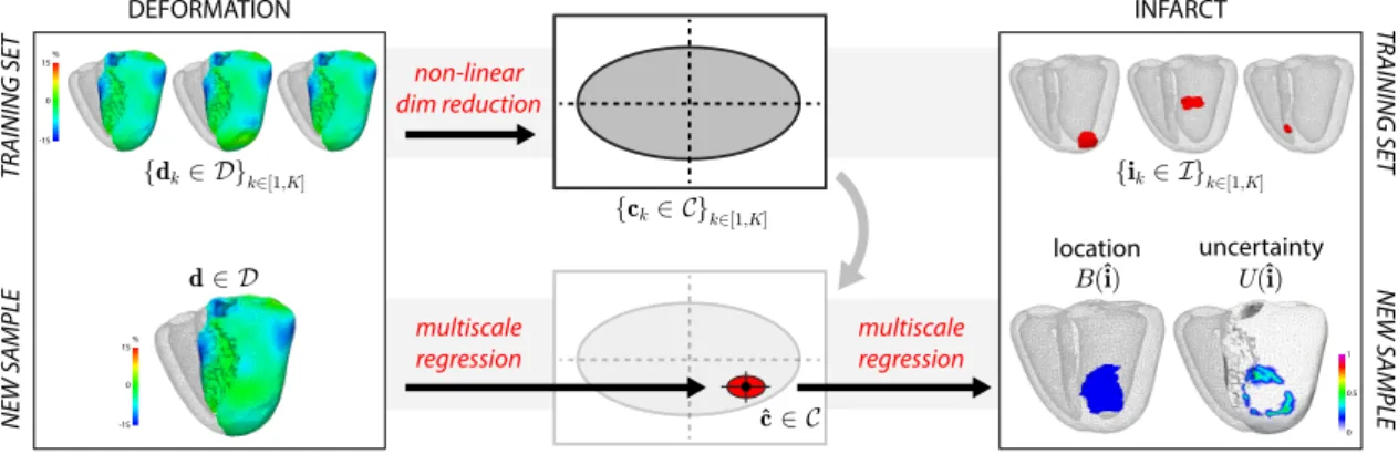
NE W SAMPLE DEFORMATION non-linear dim reduction TR AINING SET NE W SAMPLE TR AINING SET location uncertainty multiscale regression INFARCT {ck2 C}k2[1,K] d 2 D {ik2 I}k2[1,K] B(i)^ U(i)^ 0 0.5 1 -15 0 15 -15 0 15 % % c 2 C ^ {dk2 D}k2[1,K] multiscale regression
Fig. 1. Proposed pipeline to predict infarct location from local myocardial deformation and quantify the uncertainty in the prediction. discussed in Sec.IV. Deformation data are therefore treated as
a column vector of dimensions 3·Np, which corresponds to the
concatenation of the three Np-dimensional vectors encoding
the three strain components at each vertex. B. Pipeline for prediction
The processing pipeline is summarized in Fig.1, and the main variables are listed in Tab.I. Animated examples of the prediction of synthetic and real cases are available as
Supplementary Material1.
The method uses a training set composed of K pairs of
local deformation and infarct indicators, denoted {(dk 2
D, ik 2 I)}k2[1,K]. A non-linear dimensionality reduction
first provides low-dimensional coordinates {ck 2 C}k2[1,K]
from the deformation data {dk}k2[1,K]. Then, two successive
regressions are applied to the local deformation d 2 D
of a new case, and involve the pairs {(dk, ck)}k2[1,K] and
{(ck, ik)}k2[1,K]. The final outputs consist of the predicted
infarct location B(ˆi), and an estimation of the uncertainty U(ˆi) associated to it.
1) Non-linear dimensionality reduction (training set):
The (high-dimensional) local deformation data {dk 2
D}k2[1,K] are first mapped to a Euclidean space of
(low-dimensional) coordinates {ck 2 C}k2[1,K] through standard
non-linear dimensionality reduction via manifold learning.
This assumes that each high-dimensional sample dklies close
to a non-linear manifold of lower dimensionality.
To do so, we use the Isomap algorithm [29], a global method that looks for a Euclidean space where the Euclidean distance best approximates the geodesic distance along the manifold. It consists of three stages. First, a graph connects each sample
dk to a finite number of its nearest-neighbors according to
a given metric, and the graph edges are weighted by this metric. In our case, the Euclidean distance was used for the sake of simplicity. Then, the shortest path connecting each
pair (dj, dk) along the graph is computed to approximate
their geodesic distance. Squared values of this distance are stored in an affinity matrix. Finally, a centered version of this matrix is diagonalized, and the p-th component of the
1http://www-sop.inria.fr/asclepios/docs/PredictionExamples.zip
coordinates ck is defined as ck,p=p pvp,k. Here,p pis
the p-th highest eigenvalue of the centered affinity matrix, and
vp,kis the k-th component of the p-th eigenvector. The
low-dimensional embedding is simply obtained by retaining the
first components of each coordinates ck.
The method is not limited to a single choice of manifold learning algorithm. A non-linear one was retained, as unphys-iological patterns may result from linear operations on the deformation patterns [30]. Isomap was preferred over other spectral embedding [31] as no clearly separated clusters appear in the distribution of the deformation data.
2) Infarct prediction for a new subject (testing set): a) From the deformation pattern to low-dimensional co-ordinates:
The deformation pattern d 2 D of a new subject is mapped to the coordinates ˆc 2 C by kernel regression.
In a single scale formulation, this problem derives from the generic formulation of the out-of-sample extension presented in [32], which uses the Nystr¨om formula [33]. If we tolerate some dispersion of the data around the manifold, this amounts to solving the following inexact matching (details in [30]):
argmin f2F kfk 2 F+ D K X k=1 kf(dk) ckk2 ! , (1)
where k.kF stands for the norm on the reproducible kernel
Hilbert space F of functions D ! C, of kernel kD, and D
is a scalar weight balancing the adherence to the data and the smoothness of the interpolation.
This problem has an analytical solution, written as: ˆ c = f (d) = K X k=1 kD(d, dk)· ak. (2)
Here, ak is the k-th column of the matrix (KD+ 1DI) 1C,
where I is the identity matrix, C = (c1, . . . , cK)T, and KD=
(kD(di, dj))(i,j)is a kernel-based affinity matrix between the
input samples. The kernel function is defined as kD(di, dj) =
exp( kdi djk2/ 2D), D being its bandwidth.
In this work, we use a multi-scale version of the algorithm, which prevents artifacts due to non-uniformities in the density
93 94 95 96 97 98 99 100 0 0.5 1 0 1 2 3 40 50 60 70 80 90 100 10 0 20 0 0.5 1 % of vertices Bins of i
a) Synthetic data b) Real data
Bins of i
Fig. 2. Distribution of values for the infarct map ˆi, for the synthetic and real data. Errorbars indicate the median and first/third quartiles over the histograms of values in each dataset.
of the samples and automatically sets the observation scale
D. The mathematical foundations and algorithmic details for
its exact matching version are given in [34], and its inexact matching version was used in [35]. In practice, the method consists in iterating the regression algorithm from large to
small scales by setting D = T /2s, with T > 0. The
function to be interpolated at the scale s is the remainder f F(s 1), where F(s)stands for the s-th scale approximation
of the original function f, initialized as F( 1) = 0. In our
implementation [35], the starting scale s = 0 corresponds to
the overall spread of the samples: T = D2/2, where D is the
distance between the most distant pair. The procedure stops
at the resolution of the training samples: T/2s d, where d
is the average 1-NN distance over the dataset.
b) From the low-dimensional coordinates to the predicted infarct location:
A similar multiscale regression is applied to obtain an infarct map ˆi 2 I from the coordinates ˆc 2 C estimated in the
previous step. The variables ˆi, ˆc and ck now respectively
stand for ˆc, d and dk in Eq.2. The interpolating function is
now denoted g and belongs to the reproducible kernel Hilbert
space G of functions C ! I, of kernel kC. The regression
parameters have also been updated to C and C. The infarct
map therefore corresponds to ˆi = g(ˆc) = g f(d). In a single-scale formulation, it is obtained as:
ˆi = g(ˆc) =
K
X
k=1
kC(ˆc, ck)· bk, (3)
where bk is the k-th column of the matrix (KC+ 1CI) 1I,
with I = (i1, . . . , iK)T, and KC= (kC(ci, cj))(i,j).
This process is also made multiscale, with rules similar to the estimation of f in Sec.II-B2a.
c) Final prediction from the infarct map:
Due to the kernel-based formulation of the regression, the values for the infarct map ˆi are continuous, and can lie within and around the [0, 1] interval (Fig.2). Thus, they cannot be
used as such for the final prediction. A thresholding function
B is therefore applied to determine the final infarct prediction
B(ˆi). In our case, infarcts are represented by a binary value at each myocardial location. The function B therefore requires a single threshold, determined by a ROC analysis (Sec.III). C. Calculation of uncertainty
A set of possible infarct positions {B(ˆim)}m2[1,M]is
gen-erated around the prediction B(ˆi), in a three-stage process. First, M coordinates are randomly sampled from a Gaussian distribution centered on ˆc. The principal axes of this Gaussian correspond to the axes defining the space of coordinates C. The variance of the distribution is taken as a fraction
of the variance of the coordinates {ck}k2[1,K] along each
principal direction. By definition, the M samples associated to these coordinates lie on the manifold of strain patterns. Then, multiscale kernel regression is applied to each of these M coordinates, using the algorithm of Sec.II-B2b, and provides
the set of infarct maps {ˆim}m2[1,M]. Finally, these maps are
thresholded to obtain the predictions B(ˆim).
Uncertainty U(ˆi) is computed as the point-wise standard deviation over this set of M possible infarct positions.
Due to this definition, uncertainty cannot go beyond 0.5 (dimensionless units, the same as for the infarct prediction). This value corresponds to the standard deviation of a dis-crete uniform random distribution taking the values {0, 1}. In practice, an uncertainty of 0.5 at a given location means that healthy and infarcted tissue are equally probable (low confidence in the prediction). In contrast, the zone where the
M possible infarct positions overlap induces high confidence
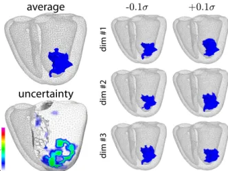
in the prediction (uncertainty close to 0). This is illustrated in Fig.3, which depicts possible infarct positions that can be generated by moving around ˆc along the principal directions of C, and the corresponding uncertainty.
Fig.4 situates our model of uncertainty with respect to iden-tified sources of uncertainty in the pipeline. Going through the space of coordinates C, of Euclidean nature, allows generating
0 0.5 1
average
-0.1¾ +0.1¾ dim #1 dim #2 dim #3uncertainty
Fig. 3. Infarct location B(ˆi) predicted from the coordinates ˆc (top left), its variations along the principal directions around ˆc (right), and corresponding uncertainty U(ˆi) (bottom left). Data correspond to test case #69 in Fig.9.
- number of samples K - graph neighborhood - metric - metric - mapping weight °D - mapping error
- number of dimensions Ndims
- metric - mapping weight °C - mapping error NE W SAMPLE DEFORMATION TR AINING SET NE W SAMPLE TR AINING SET INFARCT - threshold INFARCT map estimated location
- slices position / cut - mesh correspondence - de-MR threshold - wall + scar segmentation - physiological patterns - acquired image - mesh correspondence - features extraction - physiological patterns - acquired image - mesh correspondence - features extraction
Fig. 4. Main sources of uncertainty along the pipeline. The diagram highlights the central location of the space of coordinates to model uncertainties. a set of infarcts that are physiologically-coherent. This would
not be straightforward to achieve from a random distribution directly in the space of deformation patterns D or infarct locations I.
III. EXPERIMENTS AND RESULTS
A. Parameters setting
The number of nearest neighbors used in Isomap and the
number of dimensions Nc retained for the low-dimensional
coordinates were jointly determined. To do so, we estimated how well the embedding captures geodesic distances, depend-ing on these two variables. We computed the relative difference between the Euclidean distance in the coordinates space and the geodesic distance [30], based on [29]:
✏C(i, j) = 1 kci cjk
dN N(i, j) ,
(4)
where dN N(i, j)corresponds to the shortest path between the
pair (di, dj)along the Isomap graph. Values for the number
of nearest neighbors and number of dimensions Nc were
determined based on the median value of ✏C over the pairs
(i, j)2 [1, K]2 (Fig.5). On both synthetic and real datasets,
we retained Nc = 6, median of the value that minimizes
✏C for each nearest neighbor option. The number of nearest
neighbors was set to the value that minimizes ✏C for the
retained dimensionality (6 for both datasets).
The scalar weights used in the multiscale regression were determined as the values that minimize the median recon-struction error of the training set data, via a leave-one-out procedure. This corresponds to minimizing the
generaliza-tion ability [36], defined as GD(cj, D) = kˆcj cjk and
GC(ij, C) = kˆij ijk, where ˆcj and ˆij are reconstructed
from the K 1samples {ck}k6=j and {ik}k6=j, respectively.
Retained values were log D = 0.25, log C = 0.75
(synthetic data), and log D = 0, log C= 1.25(real data).
We set M = 500 for the uncertainty estimation, which guarantees that a 6-dimensional Gaussian distribution (the maximum dimensionality retained for the coordinates in C) is estimated with less than 10% error. This value was determined from a synthetic experiment where clouds of 6-dimensional points were randomly generated from a Gaussian distribution.
10 20 30
Number of nearest neighbors
a) Synthetic data b) Real data
40 50 20 10 30 40 50 0 0.3 Number of dimensions 10 20 30 40 50 20 10 30 40 50 0 0.45
Fig. 5. Relative difference between the Euclidean distance in the coordi-nates space and the geodesic distance (Eq.4, median value over the pairs
(i, j)2 [1, K]2). Evolution with the dimensionality and the number of nearest
neighbors, for the synthetic and real data (median over of the training set). White crosses indicate the minimum value for each nearest neighbor option. The Gaussian was centered on 0 and had distinct variances along each dimension (generated from a uniform distribution on the interval [0,1]). The Kullback-Leibler divergence for multivariate normal distributions was used to compare distribu-tions, through its convergence against the number of samples. The uncertainty parameter was set to 0.1 (10% of the total deformation data variations, expressed in the low-dimensional space). This roughly corresponds to the reproducibility of current 3D tracking reported in [37] for academic algorithms: around 3.3 ± 8.7%, 0.3 ± 1.7% and 0.4 ± 3.1% (average values over participants) for the radial, circumferential and longitudinal strain, of respective maximal amplitudes around 50, 10 and 20%. Reported ranges for commercial algorithms [38] are less comparable, as they correspond to global longitu-dinal strain from 2D sequences of a simpler synthetic dataset: between 5 and 10% for strain magnitudes around 20%. To better interpret the range of strain variations corresponding to = 0.1, we have reconstructed the strain patterns associated to the M coordinates around ˆc, and evaluated their point-wise standard deviation. This corresponds to the methodology used to estimate infarct locations, but adapted to the strain data. The variability encoded in the M coordinates was in the ranges reported in [37]: around 0.7 ± 0.2%, 0.5 ± 0.2% and 0.5±0.2% for the radial, circumferential and longitudinal strain, of respective amplitudes 9.4 ± 8.2, 13.8 ± 7.2 and
13.1± 6.4% (maximal amplitudes 38.7, 37.8 and 35.8%). The single threshold used in the function B (Sec.II-B2c) was defined as the average of the best threshold of each tested subject. These individual thresholds were determined from a ROC analysis on each tested subject, as the value that maximizes the sensitivity and the specificity in the ROC curve (Sec.III-B3a and III-C4a).
Cases were identified as outliers in the ROC analyses if their
ROC area under the curve was larger than q3+ w(q3 q1)
or smaller than q1 w(q3 q1), where w is the maximum
whisker length, and q1and q3stand for the first/third quartiles.
In our case, we set w = 1.5, which corresponds to ⇡ 99.3% coverage if the data is normally distributed (around ±2.7 times the Gaussian bandwidth).
B. Synthetic data
500synthetic cases were generated to evaluate the methods
against a large variety of infarct configurations. The cardiac function was simulated along a full cycle of duration 1 s. We used a realistic electromechanical model previously evaluated on invasive clinical data [39]. Simulations here used a single anatomical mesh from a clinical image and a fibers architecture from an atlas. Spatial correspondences between the data were therefore guaranteed.
The mesh was volumetric with tetrahedral elements, and
included the two ventricles (46876 tetrahedra and Np= 9673
vertices for the LV, of average edge length 3.4 mm, for a my-ocardial volume and mass of 173 mL and 182 g, respectively).
1) Infarct generation:
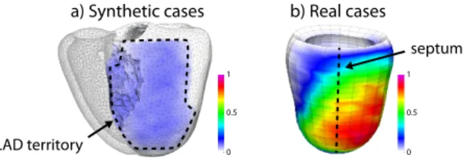
A fully-connected region corresponding to an infarct of ran-dom extent, shape, and location was constructed for each case. The algorithm determined the diseased region iteratively, as illustrated in Fig.6. It first randomly selected a starting point within the LAD coronary territory. This spatial constraint only concerns the location of the starting point, and infarcts can spread out of this territory (Fig.7a). This specific territory corresponds to the type of infarcts in the clinical database processed in this paper (Fig.7b). It also has a higher preva-lence, and better agreement exists in its delineation [40]. Here, simulated cases have the additional constraint that infarcts cannot spread over the mitral annulus.
A spherical neighborhood of random radius between 2 and 12 mm was marked as diseased, and a new starting point was randomly selected within this new region. The process was iterated a random number of times (values from
1 to 16). Infarct extent was 4.8(3.4/6.4) mL —median and
first/third quartile range, notation used throughout this paper— and corresponded to 2.8(2.0/3.7)% of the LV myocardium. Infarcts were smaller than in our clinical database (Fig.7) to test a wider variety of configurations. 400 cases were used as training set and the other 100 served as testing data.
Contractility and stiffness were altered in the zone defined by our algorithm to model local infarct (Tab.II). This partially reflects changes in active force and tissue elasticity. Only parameters with major influence on the deformation [41]
LAD territory
Iteration #1 Iteration #4 Iteration #7 Iteration #10
Fig. 6. Iterative generation of an infarct (red) with random extent, shape, and location, initiated within the LAD territory (dashed line).
septum 0 0.5 1 0 0.5 1 LAD territory b) Real cases a) Synthetic cases
Fig. 7. Average infarct location for the experiments on synthetic and real data. A colormap value of 1 at a given vertex means that 100 % of the meshes are infarcted at this location.
were altered, to keep the data into manageable amounts. The tested values corresponded to the ranges used in [42] for the construction of a validation database.
2) Deformation from electromechanical simulations: Computing the radial, circumferential and longitudinal direc-tions directly from the tetrahedral geometry of the mesh ele-ments is challenging. However, the radial direction coincides with the normal to the endocardial and epicardial surface cells. Thus, these local directions were first computed over the endocardial and epicardial surfaces. Then, these values were propagated inside the myocardium using the graph of the volumetric mesh, by iteratively setting each vertex value to the average value of its direct neighbors (10 iterations used). Strain computations used the position of the mesh vertices, including the ones internal to the wall, and did not require to also propagate the strain values inside the wall. These deformation data were spatially smoothed by a Gaussian of bandwidth 1 cm, to be closer to the clinical data resolution and to prevent inconsistencies (due to the non-homogeneity of cell sizes and orientation over the whole volumetric mesh).
3) Results:
a) ROC analysis:
A ROC analysis was performed for each subject of the testing TABLE II
PARAMETERS USED IN THE NORMAL AND SCAR ZONES(DETAILS IN[41]).
Symbol Description Units Normal Scar
0 maximum contraction Pa 3.7e6 5e4
k0 maximum stiffness Pa 6e6 1e5
katp contraction rate s 1 30 20
krs relaxation rate s 1 70 80
c1 Mooney Rivlin modulus Pa 2e4
c2 Mooney Rivlin modulus Pa 2e4
0 0.2 0.4 0.6 0.8 1 0 0.2 0.4 0.6 0.8 1
False Positive Rate = 1 - specificity
Regression Thresholding (radial strain) Thresholding (circumferential strain) Thresholding (longitudinal strain)
True Positive Rate = sensitivit
y 0 0.2 0.4 0.6 0.8 1 0 0.2 0.4 0.6 0.8 1
False Positive Rate = 1 - specificity
True Positive Rate = sensitivit
y 0 0.2 0.4 0.6 0.8 1 0 0.2 0.4 0.6 0.8 1
False Positive Rate = 1 - specificity
True Positive Rate = sensitivit
y 0 0.2 0.4 0.6 0.8 1 0 0.2 0.4 0.6 0.8 1
False Positive Rate = 1 - specificity
True Positive Rate = sensitivit
y AUC: 0.995 (0.978/0.997) AUC: 0.865 (0.819/0.905) p-value < 0.001 AUC: 0.827 (0.763/0.871) p-value < 0.001 AUC: 0.696 (0.584/0.802) p-value < 0.001
Fig. 8. ROC analysis for all the synthetic cases. Dashed traces indicate outliers. AUC: area under the curve. p-value: against the regression method.
set. The resulting set of curves is shown in Fig.8. Our method, with a median area under the curve of 0.995, significantly outperformed the thresholding of the deformation patterns computed independently for the radial, circumferential and longitudinal components of strain (0.865, 0.827 and 0.696 respectively, p < 0.001 in all cases).
Over the 100 tested cases, 13 were identified as outliers in
the ROC of the regression technique (dashed traces). Ten had small or very small infarcts, of size 0.5(0.3/0.6) mL, corre-sponding to an area under the curve of 0.890(0.827/0.939). The remaining 3 had medium to large infarcts (2.5, 2.5 and
7.1 mL), but an area under the curve > 0.905.
b) Infarct location:
After applying the thresholding function B (Sec.II-B2c), me-dian sensitivity, specificity, positive and negative predictive values were respectively 0.968, 0.977, 0.489 and 0.999. In comparison, the prediction from the average infarct map of Fig.7 (thresholded at 0.5) led to inaccurate results (no infarct predicted in all cases). Qualitatively, our method correctly predicted the infarct location in all cases, with ⇡ 1 cm margin around the infarct border, in the range of the spatial resolution of the data. This corresponded to a volume over-estimation of
4.6(3.6/5.2) mL. The average distance between the ground
truth and the prediction surfaces was 3.1(2.5/4.1) mm. Three representative outputs are shown in Fig.9. First, a case with marked strain alterations (top row), observable in all components. The uncertainty zone spreads below the infarct, where longitudinal strain in the non-scarred tissue is lower. Then, a case with a smaller infarct at the same location (middle row). Strain alterations are therefore more subtle, and higher uncertainties lie around the (mispredicted) infarct border. Finally, a case close to the septum with subtle strain alterations (bottom row), for which the inaccuracy zone and uncertainties also coincide.
c) Uncertainty quantification:
Uncertainty effectively complements the infarct prediction. Except for small infarcts, low uncertainties coincide with the ground truth infarct, while high uncertainties concentrate in the mispredicted zone. The quantitative results in Fig.10a
test case #43
test case #68
test case #29
-40 0 40 -30 0 30 -15 0 15 0 0.5 1
radial strain (%) circ. strain (%) long. strain (%) ground truth infarct predictedinfarct uncertainty
Fig. 9. Synthetic cases. Examples of strain patterns, ground truth infarct location, and infarct prediction. Top row: marked strain alterations. Middle row: subtle strain alterations due to smaller infarct size. Bottom row: subtle strain alterations due to the closeness from the septum. An animated version of the
TP FP FN TN FP TN TN FN 0 0.1 0.2 0.3 0.4 0.5 TP FP
a) Synthetic data b) Real data
Infarcted Healthy Uncertainty Uncertainty 0 0.1 0.2 0.3 0.4 0.5 0 0.05 0.1 0.15 0.2 0.25
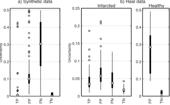
Fig. 10. Average uncertainty over the true positive, false positive, false negative and true negative vertices. Dimensionless units, the same as for the infarct prediction. Note that uncertainty cannot go beyond 0.5 (Sec.II-C). Healthy controls have no infarct: their results are only reported for the mis-predicted vertices.
confirm these qualitative observations. Almost no uncertainty results from the correctly predicted cells (true positive and true negative). In contrast, high uncertainty corresponds to the mispredicted cells (false positive and false negative).
True positive vertices with uncertainty > 0.05 mostly cor-respond to apical septal, basal anterolateral, or small infarcts. The spread of uncertainties is split over a large portion of the LAD territory in all of these cases. All the false positive vertices with uncertainty < 0.05 correspond to large infarcts, for which the overlap of the M generated infarcts is higher. In these cases, mispredicted vertices represent a small portion of the whole infarct, which is correctly located. False negative vertices with uncertainty < 0.05 are more problematic, since these locations cannot be subsequently evaluated. Two of four cases corresponded to small infarcts and were completely missed. The other two were medium/large-sized, and false negative vertices covered a small volume located in the neighboring vertices. In all of these false negative outliers, the spread of uncertainties is split over a large portion of the LAD territory and could suggest re-examination.
C. Real data
1) Infarct segmentation:
The Segment software (Medviso, Lund, SE) was used to locate the infarct in de-MR images. An experienced observer manually delineated endocardial and epicardial contours in each slice. Then, the software automatically segmented the infarct region. Manual corrections were applied if necessary. These segmentations were validated by another expert, who eventually introduced minor corrections. Their reproducibility was evaluated by repeating 5 times the segmentations of 5 different cases: the average distances between the segmented endocardial and epicardial surfaces were 1.5(1.4/1.6) mm and 1.3(1.2/1.5) mm, respectively. It has minor effect on the results, given the resolution of the volumetric meshes (Sec.III-C2).
Note that these segmentations only serve to locate the ground truth infarct for the training set and for the evaluation
of our method. If applied to a real clinical setting, the de-MR images of a new case are not required for the prediction, which only involves its deformation data and the pairs of deformation / infarct location from the training set (Fig.1).
On average, the de-MR images had a resolution of 1.56 ⇥
1.56⇥ 10.00 mm3, and 8 ± 3 slices covering the LV.
In-farct extent was 38.4(28.6/44.0) mL, and corresponded to
37.4(26.2/43.9)%of the LV myocardium.
2) Deformation from 3D echocardiographic sequences: 3D echocardiographic sequences centered on the LV were acquired in an apical view at breath-hold, via a commercially available system (iE33, Philips Medical Systems) and a broad-band wide-angle matrix-array transducer designed for har-monic contrast imaging (X3-1 probe). Images were optimized by modifying the gain, brightness, compression, and timegain compensation settings. Average frame rate and pixel size were
24 fps (heart rate: 60 bpm) and 0.65 ⇥ 0.83 ⇥ 0.57 mm3.
Myocardial strain was extracted using a prototype version of
the QLab software2. It was initialized by the landmark-based
semi-automatic segmentation of the endocardial and epicardial borders at end-diastole and end-systole, as described in [43] (5 landmarks identified: 2 on the mitral annulus of the 2- and 4-chamber views and 1 at the apex in either plane), eventually followed by manual corrections. The end-diastolic contours were propagated along the sequence by tracking the image sequences, with the constraint to pass by the end-systolic contours. Local tracking was achieved by a fast version of the demons algorithm included in the software, which tracked points inside the myocardial domain. This algorithm is detailed in [44], and evaluated in [37].
Spatial correspondence between the echocardiographic meshes was provided by the software, based on the landmarks identified for the end-diastolic and end-systolic segmentations [43], and the volumetric mesh sampling strategy described in [45]. Temporal correspondence between sequences was obtained by standard alignment techniques based on physi-ological events (in our case, start/end of the cycle and end-systole, identified as the instant of minimal volume) [7]
The volumetric meshes output by the QLab software had an average edge length of 4.8 mm, and were made of 1152
hexahedral cells and Np = 1800 vertices covering the LV.
They were defined according to the radial, circumferential and longitudinal directions. Deformation was computed along these pre-computed directions, with a resolution in the range of 1 cm. Similar to the synthetic data experiments, we limited the algorithm input to end-systolic deformation.
3) Correspondence between deformation and infarct: Spatial correspondence needed to be found between the infarct segmentation of each subject and the geometry extracted from the corresponding echocardiographic sequence, as illustrated in Fig.11. To do so, the de-MR mesh was first resampled to match the parameterization of the echocardiographic mesh. This was performed in polar coordinates centered on the long-axis of the LV. In the echocardiographic data, long-long-axis was
2http://www.healthcare.philips.com/main/products/ultrasound/technologies/
Fig. 11. Processing steps to map the infarct segmentation from the de-MR mesh (left) to the one from the echocardiographic sequence (right). defined from the apex to the center of the mitral annulus. In the
de-MR data, where slice mis-alignment may occur, it was set to connect the center of each slice segmentation. Resampling was achieved via linear interpolation, so that the meshes have the same number of points along the long-axis and along the LV circumference.
Then, spatial correspondence between the two parameteriza-tions was determined. Missing de-MR slices at the mitral ring and the apex were discarded in the echocardiographic mesh by removing the corresponding sets of points. Correspondence along the circumference was obtained from the position of the septum centerline, manually annotated in each de-MR slice and already embedded in the echocardiographic meshes.
Finally, the infarct segmentation, defined in the system of coordinates of the original de-MR mesh, was attached to the resampled de-MR mesh. This was achieved by converting the infarct segmentation into a binary image, and identifying the points of the resampled mesh that fall into the non-zero area.
0 0.2 0.4 0.6 0.8 1 0 0.2 0.4 0.6 0.8 1
False Positive Rate = 1 - specificity
Regression Thresholding (radial strain) Thresholding (circumferential strain) Thresholding (longitudinal strain)
True Positive Rate = sensitivit
y 0 0.2 0.4 0.6 0.8 1 0 0.2 0.4 0.6 0.8 1
False Positive Rate = 1 - specificity
True Positive Rate = sensitivit
y 0 0.2 0.4 0.6 0.8 1 0 0.2 0.4 0.6 0.8 1
False Positive Rate = 1 - specificity
True Positive Rate = sensitivit
y 0 0.2 0.4 0.6 0.8 1 0 0.2 0.4 0.6 0.8 1
False Positive Rate = 1 - specificity
True Positive Rate = sensitivit
y AUC: 0.909 (0.866/0.928) AUC: 0.703 (0.605/0.788) p-value < 0.001 AUC: 0.742 (0.687/0.779) p-value < 0.001 AUC: 0.610 (0.489/0.739) p-value < 0.001
Fig. 12. ROC analysis for all the real cases. Dashed traces indicate outliers. AUC: area under the curve. p-value: against the regression method.
A linear interpolator on the binary image was used to get the values at any location.
These steps substitute the use of registration techniques, which may be more challenging depending on the image qual-ity, and could be more adequate if we had no parametrization of the de-MR and echocardiographic meshes and/or no option for defining anatomical labels on these meshes.
4) Results:
a) ROC analysis:
The output of the ROC analysis is depicted in Fig.12. This analysis was only done for the infarcted cases, as healthy controls have no infarct and therefore no “positive” vertices. Similar to the synthetic data experiments, our method signifi-cantly outperformed the thresholding of the deformation pat-terns, with a median area under the curve of 0.909 (vs. 0.703,
0.742 and 0.610 respectively for the radial, circumferential
and longitudinal directions, p < 0.001 in all cases).
The possible link between baseline and follow-up infarct locations may influence the accuracy of the prediction in a leave-one-out configuration. Almost no differences were found
ground truth prediction uncertainty
0 0.5 1 test case #82 test case #48 test case #01
Fig. 13. Real cases. Top and middle rows: outliers in the ROC of Fig.12. Black arrows indicate mis-predicted regions on the lateral wall. Bottom row: healthy case with a mis-predicted infarct, accompanied by large uncertainty.
radial strain (%) circ. strain (%) long. strain (%) ground truth infarct predictedinfarct uncertainty test case #72 test case #30 test case #50 -25 0 25 septum -25 0 25 -25 0 25 0 0.5 1
Fig. 14. Real cases. Examples of strain patterns, ground truth infarct location, and infarct prediction. Top and middle rows: infarcted cases. Bottom row:
healthy volunteer correctly predicted. An animated version of the first case available as Supplementary Material1
with a leave-two-out configuration where both baseline and follow-up data of the tested subject were removed from the training set: area under the curve of 0.904(0.860/0.925), non-significant p-value.
Two outliers were identified in the ROC of the regression technique (dashed traces), and correspond to the first two cases in Fig.13. In such cases, the main infarct location —within the LAD territory— was correctly predicted. However, these cases are the only ones where part of the lateral wall is also infarcted (black arrows). This location is missed by our method, as this configuration is not represented in our training set.
b) Infarct location:
After applying the thresholding function B (Sec.II-B2c), me-dian sensitivity, specificity, positive and negative predictive values were respectively 0.828, 0.804, 0.662 and 0.927. In comparison, the prediction from the average infarct map of Fig.7 (thresholded at 0.5) reached lower performance when looking at median values over the infarcted cases (0.731, 0.897, 0.769 and 0.881, respectively). However, the limitations of this “na¨ıve” approach are hindered by the fact that in this particular database, the real cases correspond to roughly comparable infarcts. In any case, it completely fails at handling infarcts of larger variability, as for the synthetic database, or healthy subjects.
Similar to the synthetic experiments, volumes were over-estimated by our method, mainly around the infarct border:
7.7( 0.8/14.7)mL. The average distance between the ground
truth and the prediction surfaces was 3.1(2.4/4.4) mm. Three representative outputs are shown in Fig.14: two infarcted cases, for which the uncertainty zone matches the mispredicted infarct border, and a healthy case, diagnosed as such by our algorithm despite small uncertainties locally.
c) Uncertainty quantification:
Again, uncertainty complements the prediction of real infarcts (Fig.10b). True negative are associated with low uncertainties, and false positive with higher uncertainties. However, higher ambiguity exists for the other regions. The spread of uncertain-ties can be higher and overlap more the true positive region, mainly for medium infarcts. This contrasts with the results on the synthetic data, which came from a more controlled model. In the real data, the range of deformation patterns is wider, and relation between deformation and infarct is more complex. We also observe that uncertainties are lower for the real infarcts, which comes from the lower variety of infarct configurations in this database (Fig.7). Thus, the overlap of the M generated infarcts is higher, and results in lower uncertainty.
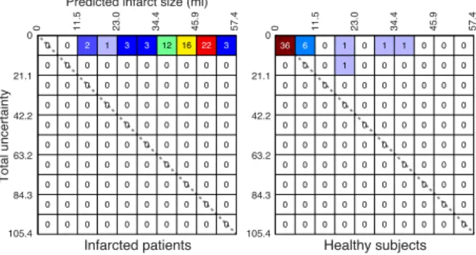
Fig.15 categorizes the studied cases depending on the size of the predicted infarct and the total uncertainty (10 ⇥ 10 bins in total). None of the 62 infarcted cases was diagnosed an infarct smaller than 17.2 mL. Almost all lie above the diagonal, meaning that uncertainty is lower in most cases and
34 3 0 1 0 1 0 0 0 0 0 0 0 0 0 0 0 0 0 0 0 0 0 0 0 0 1 0 1 0 0 0 0 0 0 0 1 0 1 1 0 0 0 0 0 0 0 0 0 0 0 0 0 0 0 0 0 0 0 0 0 0 0 0 0 1 1 0 0 0 0 0 0 0 0 0 0 0 0 0 0 0 0 0 0 0 0 0 0 0 0 0 0 0 0 0 0 0 0 0 0 0 0 0 0 0 0 0 0 0 0 0 0 0 0 0 0 0 0 0 0 0 0 0 0 0 0 0 0 0 0 0 0 0 0 0 0 0 0 2 0 0 0 0 0 1 0 2 1 1 0 0 0 0 0 1 0 1 0 0 0 0 0 1 3 5 2 0 0 0 0 0 1 0 3 9 0 0 0 0 0 0 2 5 5 3 0 0 0 0 0 1 4 8 1 0 0 0 0 0 Predicted infarct size (ml)
Infarcted patients Healthy subjects
Total uncertainty 0 11.5 23.0 34.4 45.9 57.4 105.4 84.3 63.2 42.2 21.1 0 0 11.5 23.0 34.4 45.9 57.4 105.4 84.3 63.2 42.2 21.1 0
Fig. 15. 2D histogram: number of cases vs. the predicted infarct size (10 bins) and the total uncertainty (10 bins).
36 0 0 0 0 0 0 0 0 0 6 0 0 0 0 0 0 0 0 0 0 0 0 0 0 0 0 0 0 0 1 1 0 0 0 0 0 0 0 0 0 0 0 0 0 0 0 0 0 0 1 0 0 0 0 0 0 0 0 0 1 0 0 0 0 0 0 0 0 0 0 0 0 0 0 0 0 0 0 0 0 0 0 0 0 0 0 0 0 0 0 0 0 0 0 0 0 0 0 0 0 0 0 0 0 0 0 0 0 0 0 0 0 0 0 0 0 0 0 0 2 0 0 0 0 0 0 0 0 0 1 0 0 0 0 0 0 0 0 0 3 0 0 0 0 0 0 0 0 0 3 0 0 0 0 0 0 0 0 0 12 0 0 0 0 0 0 0 0 0 16 0 0 0 0 0 0 0 0 0 22 0 0 0 0 0 0 0 0 0 3 0 0 0 0 0 0 0 0 0 Predicted infarct size (ml)
Infarcted patients Healthy subjects
Total uncertainty 0 11.5 23.0 34.4 45.9 57.4 105.4 84.3 63.2 42.2 21.1 0 0 11.5 23.0 34.4 45.9 57.4 105.4 84.3 63.2 42.2 21.1 0
Fig. 16. 2D histogram of predicted infarct size and total uncertainty, similar to the one in Fig.15, for the direct prediction from the deformation data with strain noise levels 2%.
the infarct prediction can be trusted. Among the 46 healthy subjects, 39 were diagnosed an infarct smaller than 5.7 mL (no infarct in 34 of them); all but one had low uncertainty, within the first 4 bins (34 of them showed no or almost no uncertainty). Almost all cases lie below the diagonal. The only case above the diagonal also shows medium uncertainty.
These results confirm that (i) correctly predicted cases also show low uncertainty; (ii) if the prediction indicates infarct, uncertainty may suggest carefully re-examining the case (as for the healthy case in Fig.13).
d) Usefulness of the low-dimensional space:
Our method was compared with a regression directly between the deformation and the infarct data. The experiment consisted in generating M = 500 cases around each case to predict, by adding noise on the strain data: concretely, Gaussian noise with 2% standard deviation, in the range of the reported strain errors (Sec.III-A). Then, a regression directly between the deformation and the infarct data predicted the infarct location on these M cases. Finally, uncertainty was computed as the point-wise standard deviation over this set. This direct approach was similar to our method in terms of prediction per-formance: after applying the thresholding function B, median sensitivity, specificity, positive and negative predictive values were respectively 0.800, 0.827, 0.683 and 0.924. This may be expected as both approaches combine neighbors during the regression(s): neighbors in the high-dimensional space should be roughly the same in the low-dimensional space.
However, uncertainties are not correctly represented with such a model. Noise cannot be modeled “pattern-wise” (as done through variations in the low-dimensional space in our approach) but is introduced at each spatial location, indepen-dently from the other locations. Thus, much more overlap exists between the M possible infarct positions, which induces much lower uncertainty values (Fig.16). This is rather critical, as it indicates high confidence in the prediction while inaccu-racies remain (the prediction performance is almost unchanged with respect to our approach).
IV. DISCUSSION
We presented an approach to predict an infarct location from myocardial deformation, and evaluate the local confidence in
the prediction. Methods were tested on a large database of synthetic cases obtained from a realistic electromechanical model, and real 3D echocardiographic and de-MR images.
Our method correctly predicted the infarct position in most cases, although it tended to over-estimate the exact size. Inaccuracies in the prediction of the infarct border were in the range of the resolution of the used deformation data. This systematic over-estimation can be explained by the smoothness of the deformation data, the averaging between neighbors performed in the regression, and the lack of prior on the spatial structure of the infarct. Also, our experiments on real data used de-MR images of standard quality. This means that the ground truth used for training was subject to the limited spatial resolution and contrast, which is paradoxical given our method objectives. We therefore expect the results to improve once better ground truth is available. In any case, our approach outperforms the current state-of-the-art, which provides a diagnosis at the global or regional level: in contrast, our prediction is made at each location of the myocardium. The approach is a first model towards more advanced predictions. In this sense, our objective was to demonstrate a full pipeline for reliable diagnosis, upon which improvements can be made. The uncertainty model in the coordinates space could be refined by adjusting the size of the Gaussian distribu-tion depending on the input deformadistribu-tion pattern, e.g. based on a reproducibility analysis on a representative variety of cases. Bayesian methods may offer convenient frameworks to propagate uncertainties, but require prior knowledge on the variables, which is the reason why we retained a simpler approach. Considering the infarct map ˆi before thresholding could help representing uncertainties both from the distribution of samples in the coordinates space and from the regularized regression. However, their link with a concrete uncertainty model would need to be examined. The model proposed here is more directly related to the error in the input data, which is why it was retained first for this type of prediction.
Predicting the exact infarct location is still very challenging due to the complexity of motion and deformation abnormal-ities [2]. We opted for simple descriptors of deformation that already provide a reliable prediction. Some of the strain components seem less predictive (thresholding longitudinal strain is associated to a wider variability in the ROC curves and a lower ROC area under the curve). However, we preferred to keep the prediction generic on the whole strain data. Indeed, using only the most powerful components may not be advanta-geous on all cases, and the prediction may overfit the available data. Looking at changes in deformation at other temporal phases of the cycle may increase robustness to more complex configurations (e.g. for asynchronous or reperfused hearts [2]), without necessarily including the whole temporal sequence. In particular, the quantification of post-systolic abnormalities is particularly recommended to distinguish the different ischemic substrates [2]. Complementary cardiac shape or function fea-tures could improve the accuracy of the prediction, provided they are combined in a consistent way [46]. Local thickness or curvature partially match the location of scarred tissue [1], [47]. More complete deformation measures also exist: the full strain tensor (although this requires more elaborated statistics
[48]), or blind descriptors derived from this tensor [17]. The database could be enlarged to other infarct locations. Currently, the real cases correspond to infarcts of comparable location and extent (Fig.7). This may hinder the generalization ability of the method to infarcts of more varied extents and shapes, eventually at several locations. Results on the synthetic database and healthy subjects from the real database support this observation. Once the technology is available, generating realistic synthetic images will help enriching the real database [17], [42], reducing the gap between the synthetic and real datasets, and improving the prediction. Further work will also tackle the realism of pathological simulations (e.g. by refining the tuning of the hyperelastic parameters for healthy and infarcted tissue).
Transmurality of the infarct impacts the accuracy of the prediction. By nature, infarcts initiate at the subendocardial layer, and only marked infarcts extend until the epicardium [49]. Our segmentations were checked to meet this criterion, and our algorithm could be improved to include this prior knowledge. A hidden Markov random field model was recently used to consider the spatial coherence of the infarct seg-mentation from de-MR images [50]. This improvement could be considered in further extensions of our method, although estimating the infarct position from deformation data may be more challenging to model.
Distinguishing between scarred and hibernating tissue is also challenging with our data [1]. Infarct extent is expected to decrease in revascularized cases, up to the limits of the fully scarred tissue [51]. Thus, the lack of hibernating tissue at follow-up should make infarct prediction easier. However, the scar at follow-up is harder to segment, smaller, and has broader shape variety, which hinders this supposed better performance. To consider some of these aspects, the infarct ground truth could go beyond the binary value set at each vertex, and rely on discrete or continuous values within the [0, 1] interval. In such a case, the function B (Sec.II-B2c) could be adapted to perform multiple thresholds. Our approach could also be extended to look at changes in cardiac mechanics under a stress protocol, which may improve the localization of the real scar [2], in the limits of the feasibility of the stress protocol and the availability of techniques to combine stress and rest data [46]. Subgroups of different patient stages (baseline against follow-up) or infarct types (acute against chronic) may also be trained separately, provided the size of each subgroup does not limit the robustness of the learning.
V. CONCLUSION
We have presented a new approach to predict infarct location from myocardial deformation, which goes beyond current methods for the automatic diagnosis of infarct—either achieved at the global or segmental level. A map of local uncertainty accompanies the prediction. It helps refining the diagnosis or re-examining suspicious cases. Experiments on large databases of synthetic and real cases demonstrate the reliability of the method with the radial, circumferential and longitudinal components of strain as input. Our pipeline is flexible and could be extended to more advanced measures
of cardiac shape and function, complementary sources of uncertainty, and other inference applications (e.g. predicting (ab)normal wall motion [11]).
ACKNOWLEDGMENTS
The authors acknowledge the partial support from the European Union 7th Framework Programme (VP2HF FP7-2013-611823) and the European Research Council (MedYMA ERC-AdG-2011-291080). They also thank F. Labombarda and A. Pellissier (CHU de Caen, France) who previously worked on the database collection.
REFERENCES
[1] J. Bax and V. Delgado, “Detection of viable myocardium and scar tissue,” Eur Heart J Cardiovasc Imaging, vol. 16, pp. 1062–4, 2015. [2] B. Bijnens, P. Claus, F. Weidemann, J. Strotmann, and G. Sutherland,
“Investigating cardiac function using motion and deformation analysis in the setting of coronary artery disease,” Circulation, vol. 116, pp. 2453– 64, 2007.
[3] M. Konstam, D. Kramer, A. Patel, M. Maron, and J. Udelson, “Left ventricular remodeling in heart failure: current concepts in clinical significance and assessment,” JACC Cardiovasc Imaging, vol. 4, pp. 98–108, 2011.
[4] B. Sjøli, S. Ørn, B. Grenne, H. Ihlen, T. Edvardsen, and H. Brunvand, “Diagnostic capability and reproducibility of strain by Doppler and by speckle tracking in patients with acute myocardial infarction,” JACC Cardiovasc Imaging, vol. 2, pp. 24–33, 2009.
[5] S. Roes, S. Mollema, H. Lamb, E. van der Wall, A. de Roos, and J. Bax, “Validation of echocardiographic two-dimensional speckle tracking lon-gitudinal strain imaging for viability assessment in patients with chronic ischemic left ventricular dysfunction and comparison with contrast-enhanced magnetic resonance imaging,” Am J Cardiol, vol. 104, pp. 312–7, 2009.
[6] N. Duchateau, B. Bijnens, J. D’hooge, and M. Sitges, 3D echocardiog-raphy, 2nd ed. T Shiota, ed. CRC Press, 2013, ch. Three-dimensional assessment of cardiac motion and deformation, pp. 201–13.
[7] N. Duchateau, M. De Craene, G. Piella, E. Silva, A. Doltra, M. Sitges, B. Bijnens, and A. Frangi, “A spatiotemporal statistical atlas of motion for the quantification of abnormalities in myocardial tissue velocities,” Med Image Anal, vol. 15, pp. 316–28, 2011.
[8] V. Sudarshan, U. Acharya, E. Ng, C. Meng, R. Tan, and D. Ghista, “Automated identification of infarcted myocardium tissue characterisa-tion using ultrasound images: a review,” IEEE Rev Biomed Eng, vol. 8, pp. 86–97, 2015.
[9] X. Zhang, B. Cowan, D. Bluemke, J. Finn, C. Fonseca, A. Kadish, D. Lee, J. Lima, A. Suinesiaputra, A. Young, and P. Medrano-Gracia, “Atlas-based quantification of cardiac remodeling due to myocardial infarction,” PLoS One, vol. 9, p. e110243, 2014.
[10] P. Medrano-Gracia, X. Zhang, A. Suinesiaputra, B. Cowan, and A. Young, “Statistical shape modeling of the left ventricle: myocardial infarct classification challenge,” in MICCAI-STACOM, 2015. [11] P. Medrano-Gracia, A. Suinesiaputra, B. Cowan, D. Bluemke, A. Frangi,
D. Lee, J. Lima, and A. Young, “An atlas for cardiac MRI regional wall motion and infarct scoring,” in MICCAI-STACOM, LNCS 7746, 2013, pp. 188–97.
[12] K. Wong, M. Tee, M. Chen, D. Bluemke, R. Summers, and J. Yao, “Computer-aided infarction identification from cardiac CT images: a biomechanical approach with SVM,” in MICCAI, LNCS 9350, 2015, pp. 144–51.
[13] D. Peressutti, W. Bai, W. Shi, C. Tobon-Gomez, T. Jackson, M. Sohal, A. Rinaldi, D. Rueckert, and A. King, “Towards left ventricular scar localisation using local motion descriptors,” in MICCAI-STACOM, LNCS 9534, 2016, pp. 30–9.
[14] H. Bleton, J. Margeta, H. Lombaert, H. Delingette, and N. Ayache, “Myocardial infarct localization using neighbourhood approximation forests,” in MICCAI-STACOM, LNCS 9534, 2016, pp. 108–16. [15] K. Lekadir, C. Hoogendoorn, M. Pereanez, X. Alb`a, A. Pashaei, and
A. Frangi, “Statistical personalization of ventricular fiber orientation using shape predictors,” IEEE Trans Med Imaging, vol. 33, pp. 882– 90, 2014.
[16] H. Lombaert and J. Peyrat, “Joint statistics on cardiac shape and fiber architecture,” in MICCAI, LNCS 8150, 2013, pp. 492–500.
[17] A. Prakosa, M. Sermesant, P. Allain, N. Villain, C. Rinaldi, K. Rhode, R. Razavi, H. Delingette, and N. Ayache, “Cardiac electrophysiologi-cal activation pattern estimation from images using a patient-specific database of synthetic image sequences,” IEEE Trans Biomed Eng, vol. 61, pp. 235–45, 2014.
[18] B. Burton, B. Erem, K. Potter, P. Rosen, C. Johnson, D. Brooks, and R. Macleod, “Uncertainty visualization in forward and inverse cardiac models,” in Comput Cardiol 40, 2013, pp. 57–60.
[19] E. Konukoglu, J. Relan, U. Cilingir, B. Menze, P. Chinchapatnam, A. Jadidi, H. Cochet, M. Hocini, H. Delingette, P. Ja¨ıs, M. Ha¨ıssaguerre, N. Ayache, and M. Sermesant, “Efficient probabilistic model personal-ization integrating uncertainty on data and parameters: Application to eikonal-diffusion models in cardiac electrophysiology,” Prog Biophys Mol Biol, vol. 107, pp. 134–46, 2011.
[20] D. Neumann, T. Mansi, B. Georgescu, A. Kamen, E. Kayvanpour, A. Amr, F. Sedaghat-Hamedani, J. Haas, H. Katus, B. Meder, J. Horneg-ger, and D. Comaniciu, “Robust image-based estimation of cardiac tissue parameters and their uncertainty from noisy data,” in MICCAI, LNCS 8674, 2014, pp. 9–16.
[21] L. Le Folgoc, H. Delingette, A. Criminisi, and N. Ayache, “Sparse Bayesian registration,” in MICCAI, LNCS 8673, 2014, pp. 235–42. [22] D. Peressutti, G. Penney, R. Housden, C. Kolbitsch, A. Gomez, E.
Ri-jkhorst, D. Barratt, K. Rhode, and A. King, “A novel Bayesian respira-tory motion model to estimate and resolve uncertainty in image-guided cardiac interventions,” Med Image Anal, vol. 17, pp. 488–502, 2013. [23] R. Blanc and G. Sz´ekely, “Confidence regions for statistical model based
shape prediction from sparse observations,” IEEE Trans Med Imaging, vol. 31, pp. 1300–10, 2015.
[24] V. De Luca, G. Sz´ekely, and C. Tanner, “Gated-tracking: estimation of respiratory motion with confidence,” in MICCAI, LNCS 9351, 2015, pp. 451–8.
[25] R. Moll´ero, D. Neumann, M. Roh´e, M. Datar, H. Lombaert, N. Ayache, D. Comaniciu, O. Ecabert, M. Chinali, G. Rinelli, X. Pennec, M. Ser-mesant, and T. Mansi, “Propagation of myocardial fibre architecture uncertainty on electromechanical model parameter estimation: a case study,” in FIMH, LNCS 9126, 2015, pp. 449–56.
[26] J. Caers, K. Park, and C. Scheidt, Handbook of Geomathematics. Springer Berlin Heidelberg, 2010, ch. Modeling uncertainty of complex earth systems in metric space, pp. 865–89.
[27] N. Duchateau and M. Sermesant, “Prediction of infarct localization from myocardial deformation,” in MICCAI-STACOM, LNCS 9534, 2016, pp. 51–9.
[28] J. Rossmann, C. Dym, and L. Bassman, Introduction to engineering mechanics: a continuum approach. CRC Press, 2nd edition, 2015. [29] J. Tenenbaum, V. De Silva, and J. Langford, “A global geometric
framework for nonlinear dimensionality reduction,” Science, vol. 290, pp. 2319–23, 2000.
[30] N. Duchateau, M. De Craene, G. Piella, and A. Frangi, “Constrained manifold learning for the characterization of pathological deviations from normality,” Med Image Anal, vol. 16, pp. 1532–49, 2012. [31] S. Yan, D. Xu, B. Zhang, H. Zhang, Q. Yang, and S. Lin, “Graph
embedding and extensions: a general framework for dimensionality reduction,” IEEE Trans Pattern Anal Mach Intell, vol. 29, pp. 40–51, 2007.
[32] Y. Bengio, J. Paiement, P. Vincent, O. Delalleau, N. Le Roux, and M. Ouimet, “Out-of-sample extensions for LLE, isomap, MDS, eigen-maps, and spectral clustering,” in Adv Neural Inf Process Syst 16, 2004, pp. 177–84.
[33] C. Baker, The numerical treatment of integral equations. Clarendon
Press, Oxford, 1977.
[34] A. Bermanis, A. Averbuch, and R. Coifman, “Multiscale data sampling and function extension,” Appl Comput Harmon Anal, vol. 34, pp. 15–29, 2013.
[35] N. Duchateau, M. De Craene, M. Sitges, and V. Caselles, “Adaptation of multiscale function extension to inexact matching. Application to the mapping of individuals to a learnt manifold,” in SEE-GSI, LNCS 8085, 2013, pp. 578–86.
[36] R. Davies, C. Twining, T. Cootes, and C. Taylor, “Building 3-D statistical shape models by direct optimization,” IEEE Trans Med Imaging, vol. 29, pp. 961–81, 2010.
[37] M. De Craene, S. Marchesseau, B. Heyde, H. Gao, M. Alessandrini, O. Bernard, G. Piella, A. Porras, L. Tautz, A. Hennemuth, A. Prakosa, H. Liebgott, O. Somphone, P. Allain, S. Makram Ebeid, H. Delingette, M. Sermesant, J. D’hooge, and E. Saloux, “3D strain assessment in ultra-sound (Straus): a synthetic comparison of five tracking methodologies,” IEEE Trans Med Imaging, vol. 32, pp. 1632–46, 2013.
[38] J. D’hooge, D. Barbosa, H. Gao, P. Claus, D. Prater, J. Hamilton, P. Lysyansky, Y. Abe, Y. Ito, H. Houle, S. Pedri, R. Baumann, J. Thomas, and L. Badano, “Two-dimensional speckle tracking echocardiography: standardization efforts based on synthetic ultrasound data,” Eur Heart J Cardiovasc Imaging, 2015, in press.
[39] S. Marchesseau, H. Delingette, M. Sermesant, R. Cabrera-Lozoya, C. Tobon-Gomez, P. Moireau, R. Figueras i Ventura, K. Lekadir, A. Hernandez, M. Garreau, E. Donal, C. Leclercq, S. Duckett, K. Rhode, C. Rinaldi, A. Frangi, R. Razavi, D. Chapelle, and N. Ayache, “Per-sonalization of a cardiac electromechanical model using reduced order unscented Kalman filtering from regional volumes,” Med Image Anal, vol. 17, pp. 816–29, 2013.
[40] J. Ortiz-Perez, J. Rodriguez, S. Meyers, D. Lee, C. Davidson, and E. Wu, “Correspondence between the 17-segment model and coronary arterial anatomy using contrast-enhanced cardiac magnetic resonance imaging,” JACC Cardiovasc Imaging, vol. 1, pp. 282–92, 2008.
[41] S. Marchesseau, H. Delingette, M. Sermesant, M. Sorine, K. Rhode, S. Duckett, C. Rinaldi, R. Razavi, and N. Ayache, “Preliminary speci-ficity study of the Bestel-Clement-Sorine electromechanical model of the heart using parameter calibration from medical images,” J Mech Behav Biomed Mater, vol. 20, pp. 259–71, 2013.
[42] M. Alessandrini, M. De Craene, O. Bernard, S. Giffard-Roisin, P. Allain, J. Weese, E. Saloux, H. Delingette, M. Sermesant, and J. D’hooge, “A pipeline for the generation of realistic 3D synthetic echocardiographic sequences: methodology and open-access database,” IEEE Trans Med Imaging, vol. 34, pp. 1436–51, 2015.
[43] V. Mor-Avi, C. Jenkins, H. K¨uhl, H. Nesser, T. Marwick, A. Franke, C. Ebner, B. Freed, R. Steringer-Mascherbauer, H. Pollard, L. Weinert, J. Niel, L. Sugeng, and R. Lang, “Real-time 3-dimensional echocardio-graphic quantification of left ventricular volumes: multicenter study for validation with magnetic resonance imaging and investigation of sources of error,” JACC Cardiovasc Imaging, vol. 1, pp. 413–23, 2008. [44] O. Somphone, M. De Craene, R. Ardon, B. Mory, P. Allain, H. Gao,
J. D’hooge, S. Marchesseau, M. Sermesant, H. Delingette, and E. Sa-loux, “Fast myocardial motion and strain estimation in 3D cardiac ultrasound with sparse demons,” in IEEE ISBI, 2013, pp. 1182–85. [45] Y. Zhou, O. Bernard, E. Saloux, A. Manrique, P. Allain, S.
Makram-Ebeid, and M. De Craene, “3D harmonic phase tracking with anatomical regularization,” Med Image Anal, vol. 26, pp. 70–81, 2015.
[46] S. Sanchez-Martinez, N. Duchateau, B. Bijnens, T. Erdei, A. Fraser, and G. Piella, “Characterization of myocardial motion by multiple kernel learning: application to heart failure with preserved ejection fraction,” in FIMH, LNCS 9126, 2015, pp. 65–73.
[47] D. Shah, H. Kim, O. James, M. Parker, E. Wu, R. Bonow, R. Judd, and K. RJ, “Prevalence of regional myocardial thinning and relationship with myocardial scarring in patients with coronary artery disease,” JAMA, vol. 309, pp. 909–18, 2013.
[48] X. Pennec, P. Fillard, and N. Ayache, “A Riemannian framework for tensor computing,” Int J Comput Vis, vol. 66, pp. 41–66, 2006. [49] K. Reimer and R. Jennings, “The ”wavefront phenomenon” of
myocar-dial ischemic cell death. II. Transmural progression of necrosis within the framework of ischemic bed size (myocardium at risk) and collateral flow,” Lab Invest, vol. 40, pp. 633–44, 1979.
[50] M. Viallon, J. Spaltenstein, C. de Bourguignon, C. Vandroux, A. Ammor, W. Romero, O. Bernard, P. Croisille, and P. Clarysse, “Automated quantification of myocardial infarction using a hidden Markov random field model and the EM algorithm,” in FIMH, LNCS 9126, 2015, pp. 256–64.
[51] W. Ginks, H. Sybers, and P. Maroko, “Coronary artery reperfusion. II. Reduction of myocardial infarct size at 1 week after the coronary occlusion,” J Clin Invest, vol. 51, pp. 2717–23, 1972.


![[PDF] Cours d’introduction à L'ergonomie cognitive | Cours informatique](data:image/gif;base64,R0lGODlhAQABAIAAAP///wAAACH5BAEAAAAALAAAAAABAAEAAAICRAEAOw==)