HAL Id: hal-01367977
https://hal.archives-ouvertes.fr/hal-01367977
Submitted on 18 Sep 2016HAL is a multi-disciplinary open access archive for the deposit and dissemination of sci-entific research documents, whether they are pub-lished or not. The documents may come from teaching and research institutions in France or abroad, or from public or private research centers.
L’archive ouverte pluridisciplinaire HAL, est destinée au dépôt et à la diffusion de documents scientifiques de niveau recherche, publiés ou non, émanant des établissements d’enseignement et de recherche français ou étrangers, des laboratoires publics ou privés.
How far spatial accuracy governs land-use changes
monitoring frequency: the urban sprawl monitoring
example
Jean-Pierre Chery, Jean-Stéphane Bailly, Valérie Laurent, Nathalie
Saint-Geours
To cite this version:
Jean-Pierre Chery, Jean-Stéphane Bailly, Valérie Laurent, Nathalie Saint-Geours. How far spatial accuracy governs land-use changes monitoring frequency: the urban sprawl monitoring example. Spa-tial Accuracy 2016, Jean-Stéphane Bailly, Didier Josselin, Jul 2016, Montpellier, France. pp.267-274. �hal-01367977�
How far spatial accuracy governs land-use changes monitoring frequency:
the urban sprawl monitoring example
Jean-Pierre Ch´ery*1, Jean-St´ephane Bailly2, Val´erie Laurent3, Nathalie Saint-Geours4 1AgroParisTech, TETIS, France
2AgroParisTech, LISAH, France 2Irstea, TETIS, France
4ITK, France
*Corresponding author: [email protected]
Abstract
In this paper, we illustrate how far spatial accuracy of a land-use map governs land-use changes monitoring frequency on a urban sprawl monitoring case study. From a specific Monte Carlo approach propagating uncertainties, conf4idence curves for minimal monitoring frequency to detect significant changes in urban sprawl indicators were built. Results showed that frequency decreased when uspscaling indicators but it also showed very low monitoring frequency for indicators at the lower level.
INTRODUCTION
When setting up land-use monitoring systems, spatial uncertainties and their impact on the detection of indicator changes are usually ignored. To capture a significant change in land-use indicators is thus strongly related to its spatial resolution, the velocities of the process it represents and the accuracy of the used indicators. As a consequence, the required monitoring land-use change frequency, corresponding to the mimimum time step to ensure a significant change in indicators, also depends on these three factors: indicator spatial resolution, change process velocity and spatial indicator accuracy.
In this paper, we illustrate how far spatial accuracy of a map governs land-use changes monitor-ing frequency focusmonitor-ing on urban sprawl monitormonitor-ing system from satellite imagery in southern France. Urban sprawl is a major challenge for land use planners: it causes the sealing of lands closest to the urban centers into impervious areas, thereby transforming highly productive cul-tivated soils, increasing flood hazards, fragmenting natural habitats, and raising complex issues related to transportation and social diversity. To define new urban policies, integrated moni-toring of urban sprawl is crucial. It is therefore important to choose an appropriate monimoni-toring frequency (Allen and Lu,2003). Such monitoring relies on urban sprawl indicators which suffer from uncertainties related to impervious area mapping process or from the population census methodology. In most urban sprawl monitoring studies, however, these uncertainties effects are not considered, and the monitoring frequency is chosen solely based on data availability. In practice, time lag between successive indicator calculations may range from 5 years to 25 years, or even be irregular. As for monitoring biological diversity (Yoccoz et al.,2001), having a carefully designed urban sprawl monitoring system in terms of choice of indicator, scale and temporal frequency is essential.
To support land-use planning, this paper proposes a framework to infer indicator monitoring frequencies, taking into account indicator uncertainties and scaling. This framework was
ap-plied to 3 urban sprawl indicators at municipality, inter-municipality, department, region scales on the former Languedoc-Roussillon region, France.
MATERIAL AND METHODS Study area
Languedoc-Roussillon is a former region of mainland France that covers 27,376 km2along the Mediterranean coast, and hosts about than 2.7 million inhabitants. Since the 1960s, intense population pressure in the region combined with poor urban planning led to population con-centration in the major cities and their peripheral extensions in the coastal zone. Languedoc-Roussillon region contains 1,545 municipalities aggregated in 130 inter-municipalities which facilitate cooperation on practical urban management issues, and 5 departments. Therefore, four increasing spatial supports of urban sprawl indicator were used in the study: municipali-ties, inter-municipalimunicipali-ties, departments, and entire region.
Data
Dataset of impervious polygons covers the entire study area were obtained for 1997 and 2009 from theDupuy et al.(2012) methodology, using satelitte image (RapidEye imagery for 2009) classification with numerous additive manual post-classification at 1:8,000 scale to reduce con-fusions.
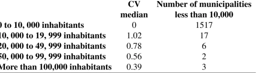
Population data for along years were taken from censuses of the French Institute of Statistics and Economic Studies (INSEE), which was performed at municipality scale. INSEE also provides uncertainty measures for their data (INSEE, 2012), as a coefficient of variation (CV) along 5 municipality categories (Tab. 1). For small municipalities having less than 10,000 inhabitants, there was exhaustive sampling and therefore, no uncertainty.
CV Number of municipalities
median less than 10,000
0 to 10, 000 inhabitants 0 1517
10, 000 to 19, 999 inhabitants 1.02 17
20, 000 to 49, 999 inhabitants 0.78 6
50, 000 to 99, 999 inhabitants 0.56 2
More than 100,000 inhabitants 0.39 3
Table 1: Median of the coefficient of variation of the number of inhabitants per municipality category (INSEE,2012), and number of municipalities of the study area in each category
Urban sprawl spatial indicators
Urban areas usually consist in namely Morphological Urban Area (MUA) obtained after mor-phological closing of a set of delineated impervious polygons. Closing consists in successive dilation and erosion (with a given radius r), allowing to merge impervious polygons. Based on the MUA,Balestrat et al.(2010) proposed a collection of spatial indicators of urban sprawl. For this study, we selected three indicators from this collection: the MUA area A (area-based), the dispersion coefficient D (shape-based) corresponding to the ratio between the cumulated areas of MUA polygons whose areas are smaller, respectively bigger than 3 hectares, and the population density P (mixing spatial and population data, i.e. number of inhabitants). Maps of these three indicators may be produced for each of the four spatial supports (municipality, inter-municipality, department, and region) (Laurent et al.,2014b).
Urban sprawl indicators uncertainty simulation
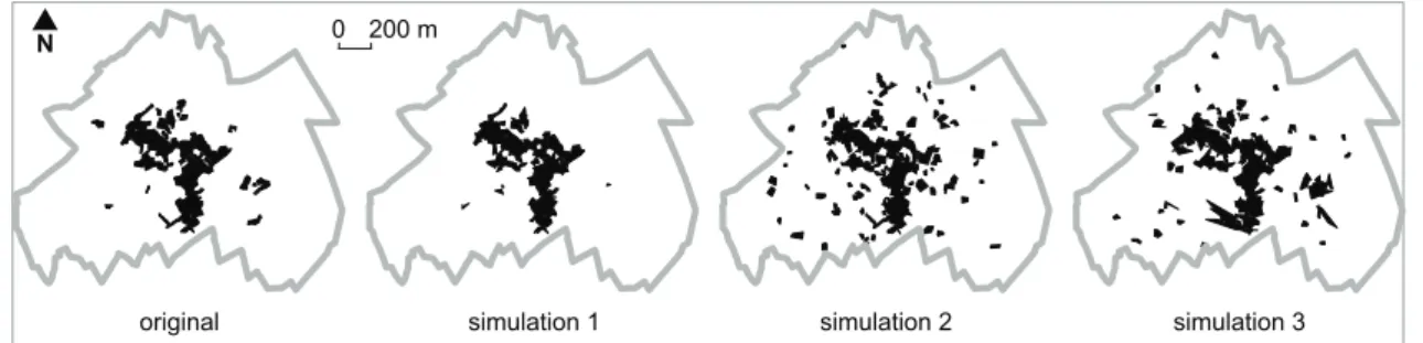
Three uncertainty sources in the computation of urban sprawl indicators A, D and P were con-sidered: i) the impervious polygons, ii) the inhabitant number per municipality, and iii) the radius r for dilatation-erosion used to build the MUA. Geometric uncertainties for both 1997 and 2009 impervious polygon layers were explicitely simulated using the approach developped
Laurent et al. (2014b). Prior to the simulation, metrics on impervious polygons geometry er-rors were first computed based on the comparison of image-processed dataset with a reference dataset on 75 sampled municipalities. These metrics quantify both the shape of impervious polygons using the position error of polygon vertices (specific spatial covariance models) and the rates of omission and commission errors of the impervious polygons within municipality areas. Based on these metrics, random realizations of impervious polygons datasets were sim-ulated for each municipality. First, the position of polygon vertices was randomly perturbed to account for geometric uncertainties. Then, small impervious polygons were randomly added or removed to account for polygon omission/commission. For more details, the reader is referred to Laurent et al.(2014a). Figure1 presents a few examples of simulated impervious polygon simulations and resulting MUA.
original simulation 1 simulation 2 simulation 3
0 200 m
N
Figure 1: Original impervious polygons from the automatic dataset and three examples of impervious polygons simulations for the municipality of Jonquieres
For each municipality, the population was assumed to follow a Gaussian distribution N (p, p ∗ CV ), where p is the municipalitys nominal population, and CV is the population coefficient of variation taken from Table1. Random realizations of population values were then drawn from N (p, p ∗ CV ).
All sources of uncertainties were propagated through the urban sprawl indicator computation chain in a Monte Carlo framework. For each value of the radius r, a Monte Carlo experiment with N = 1,000 simulations was carried out while keeping total computational cost tractable. Infering the right monitoring frequency under uncertainties
The ”right” monitoring frequency is defined here as the minimal time lag ∆tbetween two
suc-cessive indicator calculations required to detect a significant change in the indicator. It depends both on indicator uncertainty and on the magnitude of the indicator change over time. Calcu-lating ∆t is thus considered as a problem of significant differences between two independent
random variables. Let I0and I1be the indicator random variables at times t0and t1respectively,
following independent Gaussian distributions N (i0, σ) and N (i1, σ). i0 and i1 are the indicator
mean values (nominal values) at t0and t1 and σ is the indicator standard deviation, assumed to
means at a given time and a linear indicator trend with slope s, the random variable ∆T = I1−Is 0,
can be infered from the lowest significant difference (I1 − I0) at confidence level 1 − α as:
∆t=
q2σ
s (1)
where q denotes the quantile of the standard normal distribution. We can then build confidence curves for ∆t, as a function of s, for the usual confidence levels 90, 95, and 99% for instance.
To choose the range of s values for the Languedoc-Roussillon region (sLR), we calculated the
average indicator slope over the study area between 1997 and 2009, assuming similar geometric and thematic uncertainties within the 1997 and 2009 impervious polygons datasets.
RESULTS
Urban sprawl uncertainties simulation
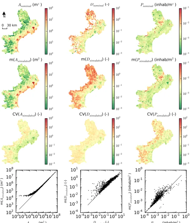
The nominal data (no uncertainty) and the simulation results at the municipality scale with 50 m radius r are presented in maps on figure2. The nominal indicator maps (line 1 - Fig.2) show the spatial patterns of the indicators. A has higher values along the coast and other plains than in the rugged inland areas. Conversely, D (dispersion coefficient) shows an opposite pattern, with higher values in the rugged inland areas, and lower values in the plains. The P (population density) map shows mostly low values with few municipalities located mostly in rugged areas having higher values Comparing the simulated indicator maps to the nominal maps, one notices that, for all three indicators, the simulated spatial patterns is similar to the nominal ones. This good match can also be seen on the scatterplots, where most points are located close to the y = x line. For A, however, the simulated values were much higher than nominal values for municipalities having A smaller than 50,000 m2. This threshold of 50,000 m2 corresponds to a rectangle MUA of 500 * 100 m, which would be an unrealistically small village. We therefore infer that the nominal map underestimates A for those municipalities. This underestimation of A by the nominal maps may be due either to the presence of clouds in the satellite images, or to the omission of (parts of) polygons in the image classification. Both D and P present a general trend to overestimation. The CV (coefficient of variation) maps contain the uncertainty information: the higher the CV value, the higher the uncertainty. The three CV maps show similar spatial trends, with lower uncertainty along the coast and in other plains, and higher uncertainties in the rugged areas. The median CV value increases from A (25 %), to P (31 %), to D (58 %), meaning that uncertainty increases from A, to P , to D. The maximum CV values were very high (2.09 for A, 6.66 for D, and 14.57 for P ), indicating locally very high uncertainties for some municipalities.
For convenience, results for other radius values are not detailly shown. Indeed, for large radius r values, more polygons are joined into the MUA, increasing A and, thereby decreasing D and P . For all three indicators, the median CV values slightly increase with increasing radius, indicating that increasing the radius slightly increases the indicator uncertainty.
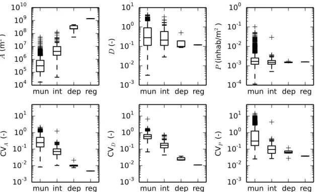
The impact of indicators spatial upscaling is shown on the boxplots of figure3. As expected, A increases with increasing entity size, because the MUA areas are being summed over larger entities. On the contrary, D decreases with increasing entity size. The entity size does not impact the P median. As expected (Heuvelink, 1998;Saint-Geours et al., 2014), for all three variables, uncertainty decreases (decreasing CV values) when upscaling. For A and D, the CV
N 0 30 km
A
nominal(m
2)
104 105 106 107 108D
nominal(-)
10−3 10−2 10−1 100 101P
nominal(inhab/m
2)
10−4 10−3 10−2 10−1m(
A
simulated) (m
2)
104 105 106 107 108m(
D
simulated) (-)
10−3 10−2 10−1 100 101m(
P
simulated) (inhab/m
2)
10−4 10−3 10−2 10−1CV(
A
simulated) (-)
10−3 10−2 10−1 100 101 102CV(
D
simulated) (-)
10−3 10−2 10−1 100 101 102CV(
P
simulated) (-)
10−3 10−2 10−1 100 101 10210
210
310
410
510
610
710
8 Anominal (m2)10
210
310
410
510
610
710
8 m( Asimu lat ed ) ( m 2)10
-410
-310
-210
-110
010
1 Dnominal (-)10
-410
-310
-210
10
-1 010
1 m( Dsim ula ted ) ( -)10
-410
-310
-210
-110
0 Pnominal (inhab/m2)10
-410
-310
-210
-110
0 m( Psimula ted ) ( inh ab /m 2)Figure 2: Results of Monte Carlo simulations, compared to the nominal results at municipality scale. The three columns present the results for the A, D, and P indicators. Line 1 shows the nominal maps, lines 2 and 3 the maps of the mean and CV respectively over the 1,000 simulations, and line 4 the scatterplots of the simulated versus nominal indicator values
values are divided by a factor 3 when upscaling from municipality to inter-municipality, by a factor 7 from inter-municipality to department, and by a factor 2 from department to region. For P , the factors are smaller: 3, 1.4, and 1.7, in the same upscaling order as for A and D.
Right monitoring frequencies
The confidence curves for the minimal monitoring time lag ∆t, as a function of the slope s of the
urban sprawl indicator trends, are presented in figure4. Looking at the A plot at municipality scale, we can see that, for all three confidence levels, the curves present a hyperbolic decreasing
mun int dep reg
10
410
510
610
710
810
910
10 A(m
2)
mun int dep reg
10
-310
-210
-110
010
1 D(-)
mun int dep reg
10
-410
-310
-210
-110
0 P(in
ha
b/m
2)
mun int dep reg
10
-310
-210
-110
010
1CV
A(-)
mun int dep reg
10
-310
-210
-110
010
1CV
D(-)
mun int dep reg
10
-310
-210
-110
010
1CV
P(-)
Figure 3: Influence of the aggregation scale on the indicator mean values and coefficients of variation (CV ). The sample sizes are: 1,545 for the municipality scale (mun), 130 for the inter-municipality scale (int), 5 for the department scale (dep), and 1 for the region scale (reg).
shape, with ∆t values starting at about 1,000 years for s close to zero, and decrease to about
10 years for s = 15% per year. This reflects the fact that smaller changes take longer than bigger changes to be detected. The curve for 99% confidence level shows higher ∆t values
than the 95%, followed by the 90% confidence level curves, reflecting the fact that to increase confidence that the detected change is a true change, and not due to uncertainties, more time is required. At municipality scale, the curves for the three indicators have similar magnitude, decreasing from 1,000 to 10 years. The magnitude of the curves decreases with upscaling, down to decreasing from 100 to 0.1 - 1. This is because the uncertainties decrease with upscaling, therefore translating into smaller ∆tvalues. The bigger the aggregation scale, the more A, P
and D drift apart in terms of ∆t values at high absolute slope values: a significant change in
A can be detected faster than a change in D, than a change in P . For all plots, even with a logarithmic y-axis, the confidence curves present a hyperbolic shape, indicating the highly non-linear relationship between s and ∆t. Looking at the particular case of Languedoc-Roussillon
for 1997-2009, the slope values are smallest for P , followed by A, and largest for D. The corresponding ∆t are therefore ranked in the opposite order, with P having the highest ∆t,
followed by A, and D having the smallest ∆t(value ranges indicated on Figure4). One should
note that, because of the logarithmic y-axis scale, the roughly constant vertical space between the confidence curves means that the difference in ∆t in years is actually much higher for
high ∆t values than for lower ∆t values. Because of averaging, the slope values decrease
when increasing the aggregation scale. Because uncertainties decrease when upscaling, ∆t
also decreases when upscaling. The 12-year time lag between the 1997 and 2009 automatic impervious polygons datasets is sufficient to detect significant differences in A and D at region and department scales, and D at inter-municipality scale, but is not sufficient for P .
1010-1 0 101 102 103 104 Mu nic ipa lity ∆ t (y ea rs) sLR: 3.0 ∆tLR: 24 - 38 A sLR: 12.7 ∆tLR: 12 - 19 D 10-1 100 101 102 103 104 sLR: 0.1 ∆tLR: 1329 - 2084 P 1010-1 0 101 102 103 Int er-mu nic ipa lity ∆ t (y ea rs) sLR: 1.8 ∆tLR: 10 - 16 sLR: 5.7 ∆tLR: 8 - 12 10-1 100 101 102 103 sLR: -0.2 ∆tLR: 107 - 167 1010-1 0 101 102 103 De pa rtm en t ∆ t (y ea rs) sLR: 1.4 ∆tLR: 1.6 - 2.5 sLR: 6.0 ∆tLR: 1.2 - 1.9 10-1 100 101 102 103 sLR: -0.1 ∆tLR: 94 - 148 0 5 10 |s| (%/year) 1010-1 0 101 102 103 Re gio n ∆ t (y ea rs) sLR: 1.5 ∆tLR: 0.6 - 1.0 99 % 95 % 90 % 0 5 10 |s| (%/year) sLR: 6.0 ∆tLR: 0.5 - 0.8 0 5 10 |s| (%/year) 10-1 100 101 102 103 sLR: -0.2 ∆tLR: 37 - 58
Figure 4: Confidence curves at 90, 95, an 99% confidence levels for the minimal monitoring time lag ∆t as a function of the absolute value of the relative slope of the indicator changes s. The slope (sLR) and time lag (∆tLR) values at 90 and 99% confidence levels for the Languedoc-Roussillon case study are indicated on the plots in the axes units
DISCUSSION
As revealed by figure 4, minimum monitoring time lags vary strongly depending on the con-sidered indicator and scale. These results are based on the average level of uncertainties for the entire Languedoc-Roussillon, whereas the uncertainties may strongly vary locally. Another caveat is that constant slope over time was assumed to build the confidence curves, and they should therefore be used with caution for inferring prospective time lag values. They are not adapted to non-linear cases, such as instantaneous abrupt growth of urban areas. Despite these limitations, we can attempt to compare the order of magnitude of the monitoring frequencies recommended by figure4to operational urban monitoring systems. In Europe, the monitoring time lag of the CORINE land cover datasets, decreased from 10 to 6 years. In the United States of America, the National Land Cover Database is updated every 5 years. These two systems are therefore appropriate for monitoring urban areas at scales as fine as the French department scale, but not inter-municipalities and municipalities. The theoretical monitoring time lag, as calculated from equation1is, of course, very important for establishing a new operational urban monitoring system, but other factors come into play. First, the theoretical time lag is different for each indicator and varies depending on the considered administrative scale. In this case study, the level of indicator uncertainty of the D indicator is simply too high to detect slight
changes. This is reinforced by the cyclic behavior of D (succession of dispersion and absorp-tion of impervious polygons in the MUA), violating the linear trend assumpabsorp-tion in the analysis. In this case, a maximum monitoring time lag has to be included to allow detecting intra-cycle changes. The time lag required for obtaining a new impervious polygon dataset is also impor-tant. Vector databases are typically updated less often than new imagery is acquired, although parts of the study area might be missing from the imagery. In addition, any governments avail-able budget and number of qualified employees may also cause practical limitations. Finally, trade-offs are required.
CONCLUSION
A specific spatially explicit Monte Carlo simulation of urban sprawl indicator was developped according to the impervious areas geometric and thematic uncertainties, socio-cultural data un-certainties and closing operation uncertianty required to obtain urban areas. This simulation process allowed to propagate and scaling uncertainties up to three urban sprawl indicators cal-culation: MUA area (A), MUA dispersion coefficient (D), and population density (P ), for the entire Languedoc-Roussillon region, France. As expected, upscaling the indicators to larger entities decreased their uncertainties. Confidence curves for minimal monitoring frequency to detect significant changes in indicator values showed that frequency decreased, for all four ad-ministrative levels. The highest frequency values were observed for the coarsest adad-ministrative scale (region), with values between 0.5 and 1 year for D and A, and 37 to 58 years for P . ACKNOWLEDGEMENTS
This work was funded by the French Research Agency in the framework of the program In-vestissements d’Avenir through the support of the GEOSUD project (ANR-10-EQPX-20). References
Allen J., Lu K. (2003). Modeling and prediction of future urban growth in the charleston region of south carolina: a gis-based integrated approach. Ecology and Society 8(2), 2.
Balestrat M., Chery J., Tonneau J. (2010). Construction of spatial indicators for decision making: interest in a participatory approach: the case of peri-urban languedoc. In Proceedings of a symposium on Innovation and Sustainable Development in Agriculture and Food, Montpellier, France, 28 June to 1st July 2010., pp. hal– 00539776. Centre de Coop´eration Internationale en Recherche Agronomique pour le D´eveloppement (CIRAD). Dupuy S., Barbe E., Balestrat M. (2012). An object-based image analysis method for monitoring land conversion
by artificial sprawl use of rapideye and irs data. Remote Sensing 4(2), 404–423.
Heuvelink G. B. (1998). Uncertainty analysis in environmental modelling under a change of spatial scale. Nutrient cycling in Agroecosystems 50(1-3), 255–264.
INSEE (2012). Recensement de la population: La prcision du chiffre de population dans les grandes communes de mtropole. Technical report, Institut National de la Statistique et des Etudes Economiques.
Laurent V., Saint-Geours N., Bailly J.-S., Chery J.-P. (2014a, July 8-11). Local urban sprawl accuracy from image segmentation uncertainties simulation. In A. Shortridge, J. Messina, S. Kravchenko, and A. Finley (Eds.), Accuracy 2014, 11th international Symposium on Spatial Accuracy Assessment in Natural Ressources and Environmental Sciences, ISARA, East Lansing, Michigan, USA, pp. 146–150.
Laurent V. C. E., Saint-Geours N., Bailly J.-S., Chery J.-P. (2014b, 21-23 may 2014). Simulating geometric uncertainties of impervious areas based on image segmentation accuracy metrics. South-Eastern European Journal of Earth Observation and Geomatics 3(2), 37–40. Special Issue: 5th GEOBIA.
Saint-Geours N., Bailly J.-S., Grelot F. (2014). Multi-scale spatial sensitivity analysis: application to a flood damage assessment model. Environmental Modelling & Software 60, 153–166.
Yoccoz N. G., Nichols J. D., Boulinier T. (2001). Monitoring of biological diversity in space and time. Trends in Ecology & Evolution 16(8), 446–453.