HAL Id: hal-00429191
https://hal.archives-ouvertes.fr/hal-00429191
Submitted on 1 Nov 2009
HAL is a multi-disciplinary open access
archive for the deposit and dissemination of sci-entific research documents, whether they are pub-lished or not. The documents may come from teaching and research institutions in France or abroad, or from public or private research centers.
L’archive ouverte pluridisciplinaire HAL, est destinée au dépôt et à la diffusion de documents scientifiques de niveau recherche, publiés ou non, émanant des établissements d’enseignement et de recherche français ou étrangers, des laboratoires publics ou privés.
Neighbourhood Broadcasting in Hypercubes
Jean-Claude Bermond, Afonso Ferreira, Stéphane Pérennes, Joseph Peters
To cite this version:
Jean-Claude Bermond, Afonso Ferreira, Stéphane Pérennes, Joseph Peters. Neighbourhood Broad-casting in Hypercubes. SIAM Journal on Discrete Mathematics, Society for Industrial and Applied Mathematics, 2007, 21 (4), pp.823-843. �hal-00429191�
Neighbourhood Broadcasting in Hypercubes
∗
Jean-Claude Bermond,
†Afonso Ferreira,
†‡St´
ephane P´
erennes
†Project MASCOTTE, CNRS - UNSA - INRIA
2004 Route des Lucioles, BP 93
F-06902 Sophia-Antipolis Cedex, France
Joseph G. Peters
§School of Computing Science
Simon Fraser University
Burnaby, British Columbia, Canada, V5A 1S6
Revised: July 2006
Abstract
In the broadcasting problem, one node needs to broadcast a message to all other nodes in a network. If nodes can only communicate with one neighbour at a time, broadcasting takes at least "log2N# rounds in a network of N nodes. In the
neigh-bourhood broadcastingproblem, the node that is broadcasting only needs to inform its neighbours. In a binary hypercube with N nodes, each node has log2N neighbours,
so neighbourhood broadcasting takes at least "log2log2(N + 1)# rounds. In this
pa-per, we present asymptotically optimal neighbourhood broadcast protocols for binary hypercubes.
Keywords: broadcasting, hypercubes, neighbourhood communication
∗This research was done while the first author was visiting Simon Fraser University
and while the fourth author was visiting Project MASCOTTE - Sophia-Antipolis.
†Supported by the European Project FET IST AEOLUS.
‡On leave from CNRS. Currently Science Officer for Telecommunications & IST at COST, Brussels. §Supported by NSERC of Canada, Universit´e de Nice - Sophia-Antipolis, CNRS, and INRIA.
1
Introduction
In the broadcasting problem, a single originator is required to disseminate a piece of infor-mation to all other nodes of a network (modelled as a graph) as quickly as possible. In the unit-cost single-port communication model, each message transmission requires one time unit or round, and each node can communicate with at most one adjacent node (neighbour) at any given time. It is well-known that broadcasting in an n-dimensional binary hypercube, or n-cube, under this model requires n = log2N rounds of communication to inform all N = 2n
nodes and that this is optimal. In this paper, we address a variant of this problem called neighbourhood broadcasting in which the originator only needs to inform its n neighbours in a hypercube. We show that this can be accomplished exponentially faster than normal (com-plete) broadcasting. A lower bound on the number of rounds for a neighbourhood broadcast is "log2(n + 1)# = "log2log2(N + 1)#. We present two neighbourhood broadcast protocols
and prove that the second protocol achieves the lower bound asymptotically. More precisely, we prove that a neighbourhood broadcast can be completed in at most log2n+!√2log2n
"
rounds (so the ratio of the upper bound for the second protocol and the lower bound tends to 1 as n tends to infinity). The exact analyses of our protocols are difficult, so, for each protocol, we introduce a sequence of truncated protocols and prove that their performances approach the lower bound.
The neighbourhood broadcasting problem was introduced by Cosnard and Ferreira [3] who outlined a simple O(log2n) protocol. They proved that the number of neighbours of the originator informed by their protocol after t rounds satisfies a Fibonacci recurrence and is proportional to (1.618)t. Thus, the number of rounds to complete a neighbourhood
broadcast using their protocol is proportional to 1.4404 log2n. In Section 2, we generalize the protocol from [3] to obtain the first of our new protocols called Protocol A. We were unable to find a closed form expression for the performance of Protocol A, but we can give generalized Fibonacci recurrence relations for truncated versions of Protocol A. The truncated protocol Ak, k ≥ 2, is obtained from Protocol A by discarding all communications
that involve a node at distance greater than k from the originator. Protocol A2is the protocol
from [3]. For Protocol A3, the number of neighbours of the originator informed after t rounds
is proportional to (1.839)t, for Protocol A
4it is proportional to (1.913)t, and for Protocol A12
it is (1.991)t.
In Section 3, we describe and analyze a more sophisticated, and more efficient, protocol called Protocol B. We show that for any fixed ! > 0 and sufficiently large t, the number of neighbours of the originator informed after t rounds of Protocol B is at least (2−!)t. We also
derive recurrence relations for the truncated protocols Bk, k ≥ 2. For example, the number of
neighbours of the originator informed after t rounds of Protocol B5is proportional to (1.999)t.
We think that Protocol B is not just asymptotically optimal, but that it is optimal or near-optimal in the sense that no protocol can inform the neighbours of the originator faster. Unfortunately, our attempts to significantly improve the lower bound have not succeeded, so improving the lower bound and determining the optimal performance exactly remain as open problems.
The protocol in Section 2 was first presented at a workshop in 1991 [1], including the closed form solution for a truncated version of the protocol and empirical evidence that the (un-truncated) protocol is asymptotically optimal. An incomplete manuscript [2] of the present paper, including the protocols in Sections 2 and 3 and parts of the analysis, has been in circulation since 1998. The workshop presentation and the manuscript have stimulated considerable interest in neighbourhood communication problems [6, 7, 10, 11, 12, 13, 16, 19, 20].
Hypercubes are Cayley graphs and many of the ideas in this paper can be modified or extended to other classes of Cayley graphs such as star graphs, which are Cayley graphs on permutation groups. The first bounds for broadcasting in star graphs appeared in [10]. The bounds were improved in [19], and an alternative protocol (with a weaker bound) was presented in [20]. The best current upper bounds for neighbourhood broadcasting in star graphs are 1.3125 log2n+ O(log2log2n) [11] and log2n+ O(#log2n) [12]. A larger class of Cayley graphs on permutation groups is studied in [16].
Neighbourhood gossiping in hypercubes, was studied in [13]. In the neighbourhood gos-siping problem, each node starts with a unique piece of information and must learn the information of all of its neighbours. Normal (complete) gossiping in an n-cube takes at least 1.44n + O(1) rounds [4, 18] and at most 1.88n + O(1) rounds [17] using half-duplex links, and exactly n rounds using full-duplex (i.e., bi-directional) links (see [14]). The bounds in [13] on the numbers of rounds, h1(n) and h2(n), for half-duplex and full-duplex neighbourhood
gossiping in an n-cube respectively, are 2.88 log2n+ O(1) ≤ h1(n) ≤ 3.76 log2n + O(1) and
h2(n) = 2 log2n+ O(1). The ideas in [13] were extended to star graphs in [10]. Note that
while the distinction between the half-duplex and full-duplex links is important for gossiping problems, it can be ignored for broadcasting problems because the (single) message in a broadcast protocol never needs to traverse any link in both directions.
In k-neighbourhood communication problems, nodes that are at distance at most k are required to communicate. The neighbourhood broadcasting and gossiping problems are examples of 1-neighbourhood communication. Bounds for k-neighbourhood broadcasting and gossiping in paths, trees, cycles, 2-dimensional grids, and 2-dimensional tori were derived in [6, 7]. The results are optimal in most cases and within an additive constant of optimal in the other cases.
There are many papers describing protocols that minimize the time for a normal (com-plete) broadcast on various interconnection networks such as hypercubes and meshes. See [15] for a discussion of models and results for broadcasting and gossiping with unit-cost models and [5, 14] for comprehensive surveys.
2
A Simple Protocol
In Cosnard and Ferreira’s neighbourhood broadcast protocol [3], the originator in a hyper-cube sends its message to a new neighbour during each round. Each informed neighbour of
the originator broadcasts to its neighbours (except the originator, of course). These neigh-bours of the neighneigh-bours do not need to know the message, but each of them can inform one new neighbour of the originator. It is not difficult to show directly that this protocol takes O(log2n) rounds to inform all neighbours of the originator in an n-cube, but we will take the opportunity to introduce some notation that we will use to analyze our new protocols.
We will identify each vertex in an n-cube by a binary string of length n. Without loss of generality, the originator is labelled with a string of n 0’s: 00 . . . 00. Each neighbour of the originator has exactly one 1 in its label. Each neighbour of a neighbour of the originator (except the originator) has two 1’s in its label. In general, a node at (Hamming) distance k from the originator has exactly k 1’s in its label. We will say that nodes at distance k from the originator are at level k. In the neighbourhood broadcasting problem, all level 1 nodes must be informed, and we want to do this as quickly as possible.
It will often be convenient to have a compact way to write node labels. When we write δ1δ2δ3δ4, δ1 < δ2 < δ3 < δ4, we mean that the label contains 1’s in the indicated positions
and 0’s in all other positions, so this is a level 4 node. The label δ1δ¯2δ3 has 1’s in positions
δ1 and δ3, a 0 in position δ2, and 0’s elsewhere, so this is a level 2 node. We will sometimes
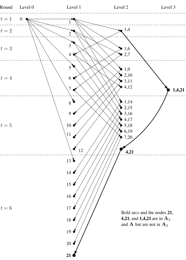
insert commas into labels to avoid ambiguity For example, 1,4,21 is the level 3 node shown in Figure 1 with 1’s in positions 1, 4, and 21.
In our figures, we will draw the originator on the left and Hamming distance from the originator will increase from left to right. When we say that a node is informed from the left or from the right, we are referring to this left to right arrangement of increasing levels.
To analyze our protocols, we use the following notation: Lt
k(P) maximum number of level k nodes informed by level k − 1 nodes
(i.e., from the left) during round t of Protocol P
Rtk(P) maximum number of level k nodes informed by level k + 1 nodes
(i.e., from the right) during round t of Protocol P Nt
k(P) = Ltk(P) + Rtk(P): maximum total number of level k nodes informed
during round t of Protocol P Tkt(P) =
t
$
i=1
Nki(P): maximum total number of level k nodes informed
during the first t rounds of Protocol P
We will often omit the name of the protocol to simplify the notation when the protocol P is clear from the context.
In the analyses of our protocols, we will show several things. For each protocol P, we will develop recurrence relations for Tt
k(P). The value of Tkt(P) is an upper bound on the
number of informed level k nodes after t rounds of Protocol P. To prove that Protocol P achieves these bounds, we need to show that it informs exactly Tt
k(P) level k nodes during
the first t rounds. We do this by showing that all newly informed nodes are distinct and that all level 1 nodes are eventually informed. We will then determine the rate at which Protocol P informs level 1 nodes as a function of t. We do this by determining the value
of the largest root ak of the associated polynomial of the recurrence relation T1t(P). The
number of level 1 nodes informed by Protocol P is proportional to at k.
We will begin by considering the protocol from [3]. We will call this Protocol A2 because
it is a truncated version of Protocol A, the first of our new protocols which we will introduce later in this section. If x is a node that is informed during round t of Protocol A2, then x
informs uninformed nodes as follows: Protocol A2 [3]
• If x is the originator, inform type L1 nodes during rounds t + 1, t + 2, . . .
• If x is a level 1 node, inform type L2 nodes during rounds t + 1, t + 2, . . .
• If x is a level 2 node, inform a type R1 node during round t + 1
The next theorem and corollary from [3] are restated using our notation. Theorem 1[3] Tt
1(A2) = T1t−1(A2) + T1t−2(A2) + 1.
Proof: First, we get Lt
1 = 1, t ≥ 1 because the originator informs one neighbour during
each round. We also have Lt
2 = T1t−1, t ≥ 2, because each level 1 node that was informed
during the first t − 1 rounds can potentially inform a new level 2 node during round t. Finally, Rt
1 = Lt−12 , t ≥ 3, because each informed level 2 node can potentially inform one
new neighbour of the originator immediately after it receives the message. Thus, Rt
1 = T1t−2,
and for t ≥ 3, we can write Tt
1 = T1t−1+ N1t = T1t−1+ L1t + Rt1 = T1t−1+ T1t−2+ 1. !
Corollary 1[3] Tt
1(A2) ∼ 1.618t.
Proof: Since T1
1 = 1 and T12 = 2, we get T1t= Ft+2−1, where Fi is the ithFibonacci number
(with starting values F1 = F2 = 1). The associated polynomial of T1t is x2− x − 1 = 0 and
its largest root is a2 = 1+ √
5
2 . It follows that the potential number of informed neighbours of
the originator after t rounds is proportional to %1+√5 2
&t
∼ 1.618t.
! To show that the bound of Theorem 1 can be attained, we need to show that every level 1 node is informed and that no nodes are informed more than once. To do this, we have to specify which nodes are informed during each round. We use the following method: During round t, the originator (which we will refer to as node 0) will inform node T1t−1+ 1
at level 1 (i.e., the node whose label has a 1 in position Tt−1
1 + 1), and any level 1 node δ,
1 ≤ δ ≤ T1t−1, that was informed during the first t − 1 rounds will inform node δ, δ + T1t+ 1
at level 2 if δ + Tt
1+ 1 ≤ n. If δ + T1t+ 1 > n, then we can assume that node δ is idle because
end of the protocol. Then, during round t + 1, each level 2 node δ, δ + Tt
1 + 1 that was
informed during round t will inform node δ + Tt
1 + 1 at level 1. Figure 1 shows how this
can be done for n ≤ T6
1 = 20. (In Figure 1, the three bold arcs and the nodes with 21 in
their labels are not part of Protocol A2 and should be ignored at this point.) The following
lemma establishes the correctness of this pattern. Lemma 1 All level 1 nodes δ with 1 ≤ δ ≤ min(n, Tt
1(A2)) are informed in t rounds.
Proof: By induction. The claim is true for t = 1 and t = 2. Now, suppose that the claim is true after round t. If n ≤ Tt
1, we are done. If n > T1t, then the new level 1 nodes
informed during round t + 1 are node Tt
1 + 1 which is informed by node 0, and all nodes δ
with Tt
1+ 2 ≤ δ ≤ min(n, T1t+ T1t−1+ 1) which are informed by the level 2 nodes δ, δ + T1t+ 1
with 1 ≤ δ ≤ Tt−1
1 . By Theorem 1, T1t+1 = T1t+ T1t−1+ 1, so the new level 1 nodes informed
during round t + 1 are all nodes δ with Tt
1 + 1 ≤ δ ≤ min(n, T1t+1). !
The first of our new protocols is a natural generalization of the protocol from [3]. Each node x that is informed during round t informs the following uninformed nodes:
Protocol A
• If x is the originator, inform type L1 nodes during rounds t + 1, t + 2, . . .
• If x is a level 1 node, inform type L2 nodes during rounds t + 1, t + 2, . . .
• If x is a level k ≥ 2 node, inform a type Rk−1 node during round t + 1 and type Lk+1
nodes during rounds t + 2, t + 3, . . .
In Protocol A, each newly informed node at level k ≥ 2 immediately informs one level k− 1 node and then informs level k + 1 nodes until the protocol terminates. The intuition is that each communication to the right can introduce a new dimension, which can eventually result in a new level 1 node being informed. So, in Protocol A, a node that has been informed from the left immediately initiates a path of communications going back to the level 1 node with the new dimension. Newly informed nodes that have received the message from the right, continue to forward the message left towards the level 1 node. Additional communications to the left will not lead directly to more informed nodes at level 1 because no new dimensions are being introduced. (We will see later in Protocol B how more new dimensions can be introduced indirectly.)
Protocol A informs level 1 nodes faster than Protocol A2. Figure 1 shows that Protocol A
can inform 21 level 1 nodes during the first six rounds while Protocol A2 can inform at most
20. The third protocol, A3, shown in Figure 1 will be described later. Protocol A3 can
inform the same number of level 1 nodes as Protocol A during the first six rounds, but eventually (when the number of rounds is nine or greater) Protocol A informs level 1 nodes faster than Protocol A3.
7,20 6,19 5,18 4,17 3,16 2,15 1,14 4,12 3,11 2,10 1,9 2,7 1,6 1,4 3 4 5 6 7 8 9 10 12 13 14 15 16 17 19 20 21 Level 3 Level 2 Level 1 Level 0 1,4,21 Round 0 1 2 11 18 4,21 1,4,21 4,21, and
Bold arcs and the nodes are in
,
21
and but are not in
t= 5 t= 2 t= 3 t= 4 t= 6 t= 1 A3 A A2
The recurrence equations for Protocol A are: Lt1(A) = 1 t ≥ 1 L12(A) = 0 Lt2(A) = t−1 $ i=1
(Li1(A) + Ri1(A)) = T1t−1(A) t ≥ 2 (1)
Ltk(A) = 0 t ≤ 2k − 3, k ≥ 2 Ltk(A) = t−2 $ i=1 (Lik−1(A) + Rik−1(A)) t ≥ 2k − 2, k ≥ 3 (2) Rtk(A) = 0 t ≤ 2k, k ≥ 1 Rtk(A) = Lt−1 k+1(A) + Rt−1k+1(A) t ≥ 2k + 1, k ≥ 1 (3) Nkt(A) = Ltk(A) + R t k(A) t ≥ 1, k ≥ 1 (4) Tkt(A) = t $ i=1 Nki(A) = t $ i=1 (Li k(A) + R i k(A)) t ≥ 1, k ≥ 1
We begin our analysis of Protocol A by simplifying the expression for Tt
1(A). We can
express Nt
1(A) as a function of the Ltk(A) by using equation (3) repeatedly:
N1t = Lt
1+ R1t = 1 + Lt−12 + Rt−12 = 1 + L2t−1+ Lt−23 + Lt−34 + · · · + Lt−k+1k + · · · . (5)
Then we use Tt
1 = T1t−1+ N1t, equation (5), and Lt−12 = T1t−2 (from equation (1)) to obtain:
T1t = T1t−1+ T1t−2+ 1 +
$
i≥3
Lt−i+1i (6)
To show that this bound for Tt
1(A) is attained by Protocol A, we have to specify which
nodes are informed during each round. We also have to show that no nodes are informed more than once, and that every neighbour of the originator is informed.
During round t, node 0 (the originator), will inform node T1t−1+ 1 at level 1. Each level
1 node δ, 1 ≤ δ ≤ Tt−1
1 , that was informed during the first t − 1 rounds will inform node
δ, δ+ Tt
1 + 1 if δ + T1t+ 1 ≤ n and will be idle if δ + T1t+ 1 > n. Once a node becomes idle,
it remains idle until the end of the protocol.
To describe the behaviour of the level 2 nodes during round t, let us rank the nodes δ1δ2,
δ1 < δ2, that are informed during the first t − 2 rounds in increasing order according to the
value of δ2. (We will prove below that there are exactly T2t−2= Lt3 such nodes and that they
all have different values of δ2.) If δ1δ2 is the jth node in this ranking, it will inform the level
To describe the pattern by which level k − 1 nodes inform level k nodes during round t (and the way that new dimensions are introduced), let us rank the level k − 1 nodes δ1δ2. . . δk−1, δ1 < δ2 < · · · < δk−1, that are informed during the first t − 2 rounds in
increasing order according to the value of δk−1. (We will prove below that there are exactly Tk−1t−2 = Lt
k such nodes and that they all have different values of δk−1.) Then, if δ1δ2. . . δk−1
is the jth node in this ranking, it will inform the level k node δ
1δ2. . . δk−1δk, where δk =
T1t+k−2+ 1 + Lt+k−2
2 + Lt3+k−3+ · · · + Lt+1k−1+ j, if δk ≤ n and will be idle otherwise.
Finally, each level k ≥ 2 node δ1δ2. . . δk, δ1 < δ2 < · · · < δk, that is informed during
round t − 1 will inform the level k − 1 node ρ1ρ2. . . ρk−1 = δ2δ3. . . δk during round t. (I.e.,
we always delete the leftmost index from the label of the level k node to obtain the label of the level k − 1 node.)
Claim 1 During round t, the nodes informed by Protocol A are:
• all level 1 nodes δ1 such that δ1 = T1t−1(A) + j, where 1 ≤ j ≤ N1t(A);
• all level 2 nodes δ1δ2, δ1 < δ2 such that δ2 = T1t(A) + 1 + j, where 1 ≤ j ≤ N2t(A);
• all level k nodes δ1δ2. . . δk, δ1 < δ2 < · · · < δk such that δk = T1t+k−2(A) + 1 +
Lt2+k−2(A) + Lt3+k−3(A) + · · · + Lt+1k−1(A) + j, where 1 ≤ j ≤ Nkt(A).
Proof: First let us prove that if the claim is true, then the level k nodes informed during round t have a different rightmost index than the nodes informed during the first t − 1 rounds, so Tt
k = ' Nkt. For level 1, it is clear that δ1 > T1t−1. The level 2 nodes informed
before round t have δ2 ≤ T1t−1 + 1 + N2t−1 and the nodes informed during round t have
δ2 ≥ T1t+ 2 = T1t−1+ N1t+ 2 = T1t−1+ Rt1+ 3 = T1t−1+ N2t−1+ 3. The level k nodes informed
before round t have δk ≤ T1t+k−3+ 1 + L2t+k−3+ · · · + Ltk−1+ Nkt−1 ≤ T t+k−2
1 and the nodes
informed during round t have δk ≥ T1t+k−2+ 2 + L t+k−2
2 + · · · + Lt+1k−1 > T t+k−2
1 .
Now suppose that the claim is true until round t − 1. We prove that the claim is true for round t by induction on t. We showed above that Tt−1
k =' Nkt−1 if the claim is true for
round t − 1. The level 1 nodes that are informed during round t are node Tt−1
1 + 1 which is
informed by the originator, and each node ρ1 = ¯δ1δ2 such that δ1δ2 is a level 2 node that was
informed during round t − 1. By the induction hypothesis, these nodes informed by level 2 nodes are of the form ρ1 = T1t−1+ 1 + j, where 1 ≤ j ≤ N2t−1. So, altogether, the level 1
nodes informed during round t are the nodes T1t−1+ j, where 1 ≤ j ≤ 1 + N2t−1 = Nt 1. This
last equation is true because Lt
1 = 1 and N2t−1 = Rt1 by equations (3) and (4).
The level 2 nodes that are informed during round t are:
• every node δ1δ2 informed by a level 1 node δ1 such that δ2 = T1t + 1 + j, where
1 ≤ j ≤ T1t−1= Lt2 (by equation 1);
• every node ρ1ρ2 informed by a level 3 node δ1δ2δ3 which was informed during round
t− 1 such that ρ2 = δ3 where ρ2 = T1t+ 1 + Lt2 + j, 1 ≤ j ≤ N3t−1 by the induction
Altogether, the level 2 nodes informed during round t are the nodes with rightmost index T1t+ 1 + j, where 1 ≤ j ≤ Lt2+ N3t−1 = Nt
2. This last equation is true because N3t−1 = R2t
and Lt
2+ Rt2 = N2t by equations (3) and (4).
The level k nodes that are informed during round t are:
• every node δ1δ2· · · δk informed by a level k − 1 node which was informed during round
t− 1 such that δk = T1t+k−2+ 1 + L j 2, where 1 ≤ j ≤ T1t−1 = L t+k−2 2 + L t+k−3 3 + · · · + Lt+1k−1+ j, 1 ≤ j ≤ Tk−1t−2= Lt k (by equation (1));
• every node ρ1ρ2· · · ρk informed by a level k + 1 node δ1δ2· · · δk+1 which was informed
during round t − 1 such that the rightmost index ρk = δk+1 satisfies ρk= T1t+k−2+ 1 +
Lt2+k−2+ Lt3+k−3+ · · · + Lt+1k−1+ j, 1 ≤ j ≤ Nk+1t−1 by the induction hypothesis.
Altogether, the level k nodes informed during round t are the nodes with rightmost index T1t+k−2+ 1 + Lt2+k−2+ Lt3+k−3+ · · · + Lt+1k−1 + j, where 1 ≤ j ≤ Lt
k+ Nk+1t−1 = Nkt. This last
equation is true because Nk+1t−1 = Rt
k and Ltk+ Rtk= Nkt by equations (3) and (4). !
If we truncate Protocol A at some level k, that is, we discard all parts of the protocol involving levels greater than k, then we get a Protocol Ak that approximates Protocol A.
In fact, Protocol A2 is exactly the protocol from [3]. Figure 1 shows the first six rounds
of Protocol A3. Notice that Protocol A3 can inform one more level 1 node than
Proto-col A2 in six rounds (using the bold arcs). The sequence A2, A3, A4, . . . is a sequence of
increasingly accurate approximations of Protocol A. We will solve the recurrence equations for Protocol Ak, but, unfortunately, we have not been able to solve the recurrence equations
for Protocol A without truncation.
Now, let us show how to find an expression for Tt
1(Ak) for the truncated protocol Ak.
First, note that for Protocol Ak we have to truncate equation (6) at level k. This is done
by deleting the terms Lt−i+1i (A) for all i > k. Our aim will therefore be to express T1t(A)
for any k as the sum of two functions, the first depending on the Lt−i+1
i (A) for i ≤ k, and
the second depending on the Lt−i+1
i (A) for i > k. Furthermore, we will show how to express
the first function as a polynomial in the T1j(A) for j ≤ t − 1. In summary, we want to obtain Tt
1(A) = Pkt+ gtk where Pkt is a polynomial in the T j 1(A)
with j ≤ t − 1 and gt
k is a function of the Lt−i+1i (A) with i > k. Therefore, for Ak we will
obtain Tt
1(Ak) = Qtk, where Q t
kis the polynomial obtained from P t
kby replacing the T j
1(A) by
the T1j(Ak), j ≤ t − 1. T1t(Ak) satisfies a generalized Fibonacci type of recurrence relation
for which the asymptotic behaviour is determined by the largest root of the associated polynomial.
For k = 2, equation (6) gives Pt
2 = T1t−1 + T1t−2+ 1 and g2t = $ i≥3 Lt−i+1i , so we obtain Tt 1(A2) = T1t−1(A2) + T1t−2(A2) + 1 which is Theorem 1.
For k ≥ 3, we have to compute the Lt−i+1
i as functions of the T j
directly, but it can be done using differences. For this purpose, we introduce a difference operator D such that for any function f (t), D[f (t)] = f (t) − f(t − 1).
Using Tt 1 = T1t−1+ D[T1t], equation (6) becomes T1t = T1t−1+ D[P2t] +$ i≥3 D[Lt−i+1i ]. (7) Using D[Pt 2] = T1t−1− T1t−3 we get T1t = P3t+ gt3 where P3t = 2T1t−1− T1t−3+ D[Lt−23 ] and g3t =$ i≥4 D[Lt−i+1i ]. (8) By (2) and (3), D[Lt−2 3 ] = Lt−23 − Lt−33 = Lt−42 + R2t−4= Rt−31 . By (4), D[Lt−23 ] = Rt−31 = N1t−3− Lt−31 = T1t−3− T1t−4− 1. (9) Using (9) in equation (8), we get Pt
3 = 2T1t−1− T1t−4− 1. This gives the following result:
Theorem 2 Tt
1(A3) = 2T1t−1(A3) − T1t−4(A3) − 1.
This is a generalized Fibonacci sequence. The largest root of the associated polynomial x4− 2x3+ 1 = 0 is a3 ≈ 1.839. Thus:
Corollary 2 Tt
1(A3) ∼ 1.839t.
We will compute the polynomials for k ≥ 4 using the following theorem: Theorem 3 Pt
k = T1t−1(A) + Pk−1t − Pk−1t−1+ T1t−3(A) − T1t−4(A) − Pk−2t−3+ Pk−2t−4, k ≥ 4.
Proof: First, we prove by induction that Pkt = T1t−1+ D[P t k−1] + Dk−2[Lt−k+1k ] and g t k = $ i≥k+1 Dk−2[Lt−i+1i ]. (10)
This is true for k = 2 by equations (1) and (6) and for k = 3 by equation (8). Suppose that it is true for k. Then using Tt
1 = T1t−1+ D[T1t], we obtain T1t= T1t−1+ D[Pkt] + Dk−1[Lt−kk+1] +
'
i≥k+2Dk−1[Lt−i+1i ], so Pk+1t = T1t−1+ D[Pkt] + Dk−1[Lt−kk+1] and gk+1t =
$
i≥k+2
Dk−1[Lt−i+1
i ].
Note that the formula of the theorem can be rewritten as
So, using equation (10), the theorem can be proved by proving that
Dk−2[Lt−k+1k ] = D[T1t−3− Pk−2t−3]. (12)
For k ≥ 3, we can use (2) and (3) to obtain D[Lt
k] = Ltk− Lt−1k = Lt−2k−1+ Rt−2k−1 = Rt−1k−2. So,
for k ≥ 4 we can use D[Lt+1k−1] = Lt−1k−2+ Rt−1k−2 to obtain
D[Ltk] = D[Lt+1k−1] − Lt−1k−2. (13)
By (13),
Dk−2[Lt−k+1k ] = Dk−2[Lt−k+2k−1 ] − Dk−3[Lt−kk−2] = D[Dk−3[Lt−k+2k−1 ] − Dk−4[Lt−kk−2]]. (14) By induction, equation (12) with k − 1 substituted for k gives
Dk−3[Lt−k+2
k−1 ] = D[T1t−3− Pk−3t−3], (15)
and equation (12) with k − 2 substituted for k and t − 3 substituted for t gives Dk−4[Lt−k
k−2] = D[T1t−6− Pk−4t−6]. (16)
Equation (11) with k − 2 substituted for k and t − 3 substituted for t gives
Pk−2t−3 = T1t−4+ D[Pk−3t−3] + D[T1t−6− Pk−4t−6]. (17) Combining equations (15), (16), and (17), we obtain
Dk−3[Lt−k+2
k−1 ] − Dk−4[Lt−kk−2] = D[T1t−3− Pk−3t−3] − Pk−2t−3+ T1t−4+ D[Pk−3t−3]
= T1t−3− Pk−2t−3. !
Using Theorem 3, we are able to compute all of the polynomials Pt
k for k ≥ 4 and
therefore the recurrence relations for Tk
1(Ak). For example, we obtain:
Theorem 4 Tt 1(A4) = 3T1t−1(A4)−2T1t−2(A4)+T1t−3(A4)−3T1t−4(A4)+T1t−5(A4)+T1t−6(A4). Theorem 5 Tt 1(A5) = 4T1t−1(A5) − 5T1t−2(A5) + 4T1t−3(A5) −7Tt−4 1 (A5) + 6T1t−5(A5) − T1t−8(A5).
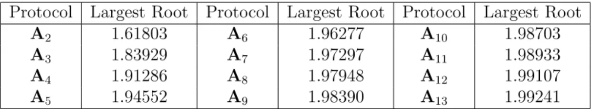
The following table shows the value of the largest root ak of the associated polynomial
of Tt
1(Ak) for k ≤ 13. The number of level 1 nodes informed by Protocol Ak is proportional
to at k.
Protocol Largest Root Protocol Largest Root Protocol Largest Root
A2 1.61803 A6 1.96277 A10 1.98703
A3 1.83929 A7 1.97297 A11 1.98933
A4 1.91286 A8 1.97948 A12 1.99107
A5 1.94552 A9 1.98390 A13 1.99241
Table 1: Asymptotic Values for Protocol Ak.
3
A Sophisticated Protocol
In Protocol A, each newly informed node at level k ≥ 3 only informs one level k − 1 node before broadcasting to the right. This leaves some nodes at levels 2 through k−1 uninformed. The idea of our second protocol, Protocol B, is to inform as many nodes as possible at the lower levels, because these nodes can introduce new dimensions by communicating to the right and this will lead to new level 1 nodes. A new dimension introduced by a level k node in a communication during round t can result in a newly informed node at level 1 as early as round t + k.
To describe Protocol B more precisely, we need to extend the notation used for Pro-tocol A. We will distinguish nodes informed from the right by a node x according to the number of communications to the left that have been made by x. If x is a node at level k, then the first node that it informs at level k − 1 is a type Rk−1,1 node, the second node that
it informs at level k − 1 is a type Rk−1,2 node, and so on. This gives the following notation:
Lt
k(P) maximum number of level k nodes informed by level k − 1 nodes
during round t of Protocol P Rt
k,1(P) maximum number of level k nodes informed during round t of
Protocol P by level k + 1 nodes which have not communicated to the left before round t
Rtk,j(P) maximum number of level k nodes informed during round t of Protocol P by level k + 1 nodes which have informed exactly j− 1 level k nodes before round t
Rtk(P) =
k
$
j=1
Rtk,j(P): maximum total number of level k nodes informed
by level k + 1 nodes during round t of Protocol P Nt
k(P) = Ltk(P) + Rtk(P): maximum total number of level k nodes informed
during round t of Protocol P Tt
k(P) =
t
$
i=1
Nki(P): maximum total number of level k nodes informed during the first t rounds of Protocol P
t, then x informs the following uninformed nodes: Protocol B
• If x is the originator, inform type L1 nodes during rounds t + 1, t + 2, . . .
• If x is a level 1 node, inform type L2 nodes during rounds t + 1, t + 2, . . .
• If x is a type Lk node, k ≥ 2, inform a type Rk−1,1 node during round t + 1, a type
Rk−1,2 node during round t + 2, . . . , a type Rk−1,k−1 node during round t + k − 1, and type Lk+1 nodes during rounds t + k, t + k + 1, . . .
• If x is a type Rk,j node, k ≥ 2, 1 ≤ j ≤ k, inform a type Rk−1,j node during round
t+ 1, a type Rk−1,j+1 node during round t + 2, . . . , a type Rk−1,k−1 node during round t+ k − j, and type Lk+1 nodes during rounds t + k − j + 1, t + k − j + 2, . . .
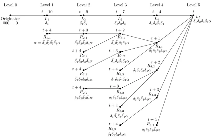
Before we analyze Protocol B, it will be helpful to look at an example of part of the protocol. Figure 2 shows a path from the originator to a level 5 node labelled δ1δ2δ3δ4α.
The tree of all communications to the left from node δ1δ2δ3δ4α is also shown, but all other
communications have been omitted to keep the figure simple. In our example, dimension α is introduced in the communication right from node δ1δ2δ3δ4 to node δ1δ2δ3δ4αduring round t.
The rounds during which other nodes are informed and the types of the nodes are indicated in the figure.
Figure 2 illustrates some properties that we will use in our analysis. First, consider the path of type Lk nodes from the originator to node δ1δ2δ3δ4α along the top of the diagram.
Each of the communications to the right shown in the figure introduces a new dimension, but the rounds during which these communications occur are not consecutive because commu-nications to the left by the type Lk nodes are done before communications to the right. The
type L2 node labelled δ1δ2 makes one communication to the left (to a type R1,1 node) before
informing the type L3 node δ1δ2δ3, the type L3 node makes two communications to the left,
and in general, a type Lk node, k ≥ 2, will make k − 1 communications to the left before
communicating to the right. So, a type Lk node will receive the message k−1
$
i=1
i = k(k − 1) 2 rounds after the originator initiates the path to the right.
Next, we can consider node δ1δ2δ3δ4αto be the root of a broadcast tree, which we denote
Tδ1δ2δ3δ4α, going left and starting in round t + 1. The tree Tδ1δ2δ3δ4α, is a complete binomial
tree of depth 4 and contains all nodes at levels 1 through 5 with a 1 in position α. Notice that the number of level i+1 nodes in Tδ1δ2δ3δ4αis
(
4i
)
, 1 ≤ i+1 ≤ 5. In particular, Tδ1δ2δ3δ4α
contains one new level 1 node. Another useful property of Tδ1δ2δ3δ4α is that all
4 $ i=0 *4 i + = 24 nodes, including δ1δ2δ3δ4α, finish their communications to the left during the same round
L5 L3 L2 L1 L4 Originator Level 5 Level 4 Level 3 Level 2 Level 1 Level 0 R3,3 R3,2 R2,1 R2,2 R2,2 R2,2 R1,1 δ1δ2δ3δ4 δ1δ2δ3 δ1δ2 δ1 000 . . . 0 t + 4 t + 3 t + 2 t + 1 t + 4 δ1δ2δ3δ4α ¯ δ1δ¯2δ3δ4α R3,1 R4,1 ¯ δ1δ2δ3δ4α R3,2 ¯ δ1δ¯2δ3δ¯4α ¯ δ1δ2δ¯3δ¯4α δ¯1δ2δ3δ¯4α δ1δ¯2δ3δ4α t + 2 R4,3 ¯ δ1δ¯2δ¯3δ4α δ1δ¯2δ¯3δ¯4α R4,4 δ1δ2δ3δ¯4α t + 3 δ1δ2δ¯3δ4α R4,2 t + 3 t + 4 t + 4 t + 4 ¯ δ1δ2δ¯3δ4α t + 4 δ1δ2δ¯3δ¯4α R3,3 t + 3 δ1δ¯2δ¯3δ4α t + 4 t + 4 R3,3 δ1δ¯2δ3δ¯4α α = ¯δ1δ¯2δ¯3δ¯4α t− 9 t− 10 t− 7 t− 4 t
Figure 2: The broadcast tree of Tδ1δ2δ3δ4α
these communications to the right introduces a new dimension, and each node that receives the message from the left during round t + 5 is the root of a broadcast tree going left that contains a new level 1 node. In general, the broadcast tree of a type Lknode that is informed
during round t contains 2k−1 nodes, including one level 1 node that is informed during round
t+ k − 1, and all nodes of this tree communicate to the right during round t + k introducing 2k−1 new dimensions.
With this intuition, we can write the recurrence equations for Protocol B: Lt1(B) = 1 t ≥ 1 Ltk(B) = 0 t ≤ k(k − 1) 2 , k≥ 2 Ltk(B) = t−k+1 $ i=1 Lik−1(B) + k−1 $ j=1 t−k+j $ i=1 Rik−1,j(B) t ≥ k(k − 1) 2 + 1, k ≥ 2 (18) Rtk,j(B) = 0 1 ≤ k < j Rtk,j(B) = 0 t ≤ k(k + 1) 2 + j, 1 ≤ j ≤ k Rtk,j(B) = Lt−jk+1(B) + j $ i=1 Rt−j+i−1k+1,i (B) t ≥ k(k + 1) 2 + j + 1, 1 ≤ j ≤ k (19) Rtk(B) = 0 t ≤ k(k + 1) 2 + 1, k ≥ 1 Rtk(B) = k $ j=1 Rtk,j(B) t ≥ k(k + 1) 2 + 2, k ≥ 1 Nkt(B) = Ltk(B) + Rkt(B) t ≥ 1, k ≥ 1 Tkt(B) = t $ i=1 Nki(B) = t $ i=1 (Lik(B) + R i k(B)) t ≥ 1, k ≥ 1
Theorem 6 Protocol B informs 2t level 1 nodes no later than round t +,√8t+1−1 2
-.
Proof: During each round of Protocol B, each informed node informs an uninformed neigh-bour, so the total number of informed nodes after t rounds is 2t. By equation (18), the
most distant informed node from the originator after t rounds is at level at most kt where
t≤ kt(kt+1) 2 . So, kt = ,√ 8t+1−1 2 -.
From the discussion above, a type Lknode x that is informed during round t is the root of
a broadcast tree Txwith 2knodes that are all informed during round t + k − 1. In particular,
Tx includes a level 1 node which we will call f1(x).
Now we will show that at time t + kt there are at least 2t informed level 1 nodes. To
prove this, we will associate with each of the 2t nodes informed during the first t rounds, a
level 1 node that is informed no later than round t + kt.
If node x is of type Lt!
k, the associated level 1 node is f1(x) of the broadcast tree Tx, and
If node x is of type Rm, it belongs to the broadcast tree of a type Lt−hk node r(x) with
k ≤ kt; therefore m ≤ kt− 1.
Case 1: If h ≥ k − 1, then all the nodes of the broadcast tree of r(x) are informed during round t. During round t + 1, x will inform a type Lt+1
m+1 node y, which in turn informs the
level 1 node f1(y) m rounds later, that is, during round t + m + 1 ≤ t + kt.
Case 2: If h < k − 1, then only 2h − 1 nodes of the broadcast tree of r(x) are informed during the first t rounds. We will show that we can associate at least 2h
− 1 informed level 1 nodes with this broadcast tree. Indeed, all the nodes of the broadcast tree of r(x) are informed during round t − h + k − 1. During round t − h + k, any type Rp node of the
broadcast tree will inform a type Lp+1 node which in turn informs a level 1 node during
round t − h + k + p. So, no later than round t + kt we have at least as many informed
level 1 nodes as the number of Rp nodes with p ≤ h. The number of such Rp nodes is
1 +(k−1 1 ) + · · · + (h−1k−1) > 1 + ( h 1) + · · · + ( h h−1) = 2 h − 1. !
Corollary 3 In the hypercube with N = 2n nodes, neighbourhood broadcasting can be done
in at most log2n+!√2log2n" rounds.
Corollary 4 For any fixed ! > 0 and sufficiently large t, the number of level 1 nodes in-formed by Protocol B in t rounds is at least (2 − !)t.
Proof: After t = u +√2u + 1 rounds, we have 2u level 1 nodes informed. Solving for u we
get u = t + 1 −√2t + 1. So, at time t there are at least 2t+1−√2t+1 informed level 1 nodes.
For any fixed ! and sufficiently large t, 2t+1−√2t+1 ≥ (2 − !)t.
! We can truncate Protocol B at some level k ≥ 3, in the same way that we truncated Protocol A, to get a sequence B3, B4, B5, . . . , of increasingly accurate approximations of
Protocol B. Protocol B2 is exactly the same as Protocol A2. We begin our analysis in the
same way as we did for Protocol A (cf. equation `(6)) by simplifying the expression for Tt 1(B):
T1t = Tt−1
1 + N1t= T1t−1+ 1 + Lt−12 + Lt−23 + · · · + Lt−k+1k + · · · .
Noting that Lt−12 = T1t−2, we get T1t = T1t−1+ T1t−2+ 1 +$
i≥3
Lt−i+1i . (20)
Using the difference operator with equation (18), we get D[Lt k] = Lt−k+1k−1 + k−1 $ j=1 Rt−k+jk−1,j .
By repeated use of equation (19), we get D[Lt 3] = Lt−22 + 2Lt−33 + 3Lt−44 + · · · + (i − 1)Lt−ii + · · · , (21) D[Lt 4] = Lt−33 + 3Lt−44 + 6Lt−55 + · · · + *i − 1 2 + Lt−ii + · · · , (22)
and more generally D[Lt k] = $ i≥k−1 * i − 1 k− 2 + Lt−ii . (23) Theorem 7 T1t(B3) = 2T1t−1(B3) + T1t−3(B3) − 2T1t−4(B3) − T1t−5(B3) − 2.
Proof: Truncating equation (20) at level 3 gives T1t = Tt−1
1 + T1t−2+ 1 + Lt−23 . (24)
Applying the difference operator to (24) we get Tt
1 = T1t−1+ D[T1t] = 2T1t−1− T1t−3+ D[Lt−23 ].
By (21), D[Lt−2
3 ] = Lt−42 + 2Lt−53 = T1t−5+ 2Lt−53 , so we get
T1t = 2T1t−1− T1t−3+ T1t−5+ 2Lt−53 . (25)
Substituting t − 3 for t in equation (24) gives Lt−53 = T1t−3− (T1t−4+ T1t−5+ 1) and so (25)
becomes Tt
1 = 2T1t−1+ T1t−3− 2T1t−4− T1t−5− 2. !
Corollary 5 Tt
1(B3) ∼ 1.913t.
It is interesting to note that Tt
1(B3) = T1t(A4) (compare Theorems 7 and 4) even though
the protocols are different. The originator and nodes of types L1 and L2 behave the same
in the two protocols. In Protocol A4, each level 3 node informs a type R2,1 node and then
informs level 4 nodes until the end of the protocol. Each level 4 node informs one level 3 node and then becomes idle. In Protocol B3, each level 3 node informs a type R2,1 node and
a type R2,2 node and then becomes idle. The type R2,1 nodes behave the same in the two
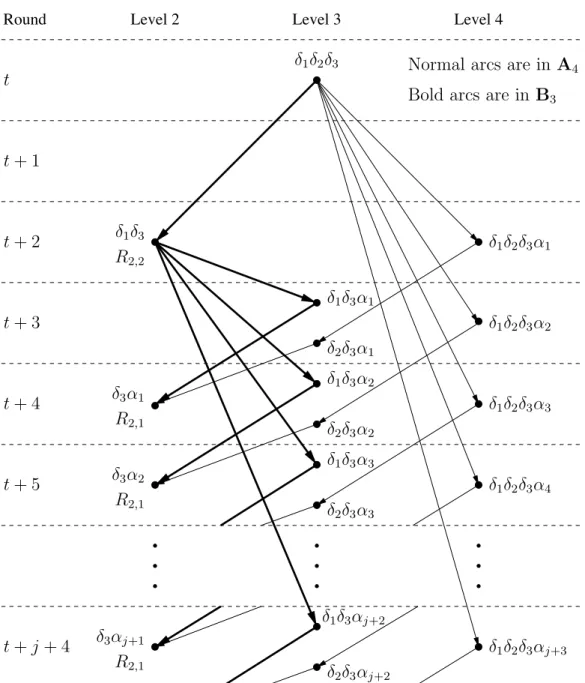
protocols. To see that the two protocols inform the same level 1 nodes during each round, we will compare the parts of the protocols that are different. Figure 3 shows parts of the broadcast trees rooted at a level 3 node δ1δ2δ3. In both protocols, node δ1δ2δ3 informs the
type R2,1 node δ2δ3 during round t + 1. Node δ2δ3 behaves the same in both protocols, so
it is not shown. In the figure, communications that are in Protocol A4 are shown in normal
typeface and communications that are in Protocol B3 are shown in bold typeface. Notice
that the two protocols inform different level 3 nodes, but the same level 2 nodes are informed. In both protocols, node δ3α1 will inform the new level 1 node α1 during round t + 5, node
δ3α2 will inform the new level 1 node α2 during round t + 6, and so on.
Level 4 Level 3 Level 2 Round δ1δ2δ3αj+3 δ1δ2δ3α4 δ1δ2δ3α3 δ1δ2δ3α2 δ1δ2δ3α1 δ3α1 δ1δ3 δ1δ3α1 δ1δ2δ3 δ1δ3αj+2
Bold arcs are in B3
Normal arcs are in A4
t t+ 1 t+ 2 t+ 3 t+ 4 t+ 5 t+ j + 4 δ3αj+1 R2,1 δ3α2 R2,1 R2,1 R2,2 δ2δ3αj+2 δ2δ3α3 δ1δ3α3 δ2δ3α2 δ1δ3α2 δ2δ3α1
Figure 3: Differences between Protocols A4 and B3.
Theorem 8 Tt 1(B4) = 3T1t−1(B4) − 2T1t−2(B4) + T1t−3(B4) − 5T1t−5(B4) +T1t−6(B4) + 3T1t−8(B4) + T1t−9(B4) + 3. Corollary 6 Tt 1(B4) ∼ 1.9867t. Theorem 9 Tt 1(B5) = 4T1t−1(B5) − 5T1t−2(B5) + 3T1t−3(B5) − T1t−4(B5) − T1t−5(B5) −6Tt−6 1 (B5) + 7T1t−7(B5) − T1t−8(B5) + 4T1t−9(B5) + 7T1t−10(B5) −4T1t−11(B5) − 2T1t−12(B5) − 4T1t−13(B5) − T1t−14(B5) − 4. Corollary 7 T1t(B5) ∼ 1.9989t.
4
Conclusions
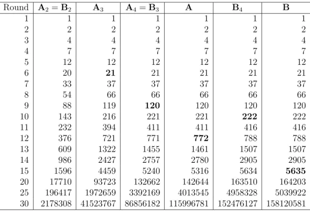
The following table shows the numbers of informed level 1 nodes for several protocols. These numbers were obtained using programs based on the recurrence relations in this paper. The numbers for the truncated protocols can also be obtained using the theorems in this paper. The protocols in Table 2 are ordered left to right according to increasing number of informed level 1 nodes. An entry shown in bold font indicates the first round during which a protocol is better than the protocol on its left.
Round A2 = B2 A3 A4 = B3 A B4 B 1 1 1 1 1 1 1 2 2 2 2 2 2 2 3 4 4 4 4 4 4 4 7 7 7 7 7 7 5 12 12 12 12 12 12 6 20 21 21 21 21 21 7 33 37 37 37 37 37 8 54 66 66 66 66 66 9 88 119 120 120 120 120 10 143 216 221 221 222 222 11 232 394 411 411 416 416 12 376 721 771 772 788 788 13 609 1322 1455 1461 1507 1507 14 986 2427 2757 2780 2905 2905 15 1596 4459 5240 5316 5634 5635 20 17710 93723 132662 142644 163510 164203 25 196417 1972659 3392169 4013545 4958328 5039922 30 2178308 41523767 86856182 115996781 152476127 158120581
Table 2: Level 1 Nodes Informed.
It is interesting to examine the last row of Table 2 which shows the numbers of informed nodes after 30 rounds. Protocol A3nearly doubles the number of informed nodes compared to
Protocol A2, and Protocol A4 more than doubles it again. Protocol B is so much better than
Protocol A that even the truncated Protocol B4 outperforms the untruncated Protocol A.
We know from Corollary 4 that Protocol B is asymptotically optimal. The last two columns suggest that Protocol B4 is almost as good as the untruncated Protocol B. To examine this
further, we used programs based on the recurrence relations to determine lower bounds on the rates that the truncated protocols inform level 1 nodes. More precisely, the number of level 1 nodes informed by each truncated Protocol Ak is proportional to atk where ak
is the largest root of the associated polynomial of Tt
1(Ak). Similarly, the performance of
Protocol Bk is proportional to btk where bk is the largest root of associated polynomial of
Tt
1(Bk). The results are shown in Figure 4. The lower curve shows the sequence {ak},
omitted the value a2 = b2 = 1+ √
5
2 ≈ 1.618 for Protocol A2 = Protocol B2 to reduce the
range of the vertical scale of the graph.) The graph shows that the sequence {bk} converges
very quickly with increasing k towards the optimal value 2 (shown as a horizontal line at the top of the graph). The sequence {ak} converges more slowly, but it is clear that it is also
approaching the optimal value.
1.92 1.84 2.00 1.96 1.88 20 12 8 4 16
Figure 4: Asymptotic Convergence of Largest Roots ak and bk for k ≥ 3.
An alternative approach to solving the recurrence relations in this paper is to use the matrix approach described in [8, 9]. We have applied this approach to the protocols in this paper and obtained the same polynomials for the truncated protocols.
We note that the recurrence relations that we have presented in this paper apply to k-neighbourhood broadcasting for any k ≥ 1. It is possible to extend our analysis to determine expressions for the truncated protocols for k > 1, but the derivations might be quite long.
Finally, we re-iterate that improvement of the lower bound for neighbourhood broad-casting or a proof that no protocol can inform the neighbours of the originator faster than Protocol B are open problems.
References
[1] J.-C. Bermond, A. Ferreira, and J.G. Peters. Partial broadcasting in hypercubes. Inter-national Workshop on Interconnection Networks (IWIN), Luminy, France, July 1991. [2] J.-C. Bermond, A. Ferreira, S. P´erennes, and J.G. Peters. Neighbourhood broadcasting
in hypercubes. Manuscript, August 1998.
[3] M. Cosnard and A. Ferreira. On the real power of loosely coupled parallel architectures. Parallel Processing Letters 1: 103–111, 1991.
[4] S. Even and B. Monien. On the number of rounds necessary to disseminate information. Proc. 1st ACM Symp. on Parallel Algorithms and Architectures, Santa Fe, New Mexico:
318–327, June 1989.
[5] P. Fraigniaud and E. Lazard. Methods and problems of communication in usual net-works. Discrete Applied Mathematics 53: 79–133, 1994.
[6] G. Fertin and A. Raspaud. k-neighborhood broadcasting. Proc. International Collo-quium on Structural Information and Communication Complexity (SIROOCO 8), Vall de N´uria, Spain, June 2001. Proceedings in Informatics 11, Carleton Scientific (2001), 133–146.
[7] G. Fertin and A. Raspaud. Neighborhood communications in networks. Proc. Euro-conference on Combinatorics, Graph Theory and Applications (COMB01), Barcelona, Spain, September 2001. Electronic Notes on Discrete Mathematics 10, Elsevier (2001). [8] M. Flammini and S. P´erennes. On the optimality of general lower bounds for
broad-casting and gossiping. SIAM Journal on Discrete Mathematics 14: 267–282, 2001. [9] M. Flammini and S. P´erennes. Lower bounds on the broadcasting and gossiping time
for restricted protocols. SIAM Journal on Discrete Mathematics 17: 521–540, 2004. [10] S. Fujita. Neighborhood information dissemination in the star graph. IEEE Transactions
on Computers 49: 1366–1370, 2000.
[11] S. Fujita. Time-efficient multicast to local vertices in star interconnection networks under the single-port model. IEICE Transactions on Information and Systems E87-D: 315–321, 2004.
[12] S. Fujita. Optimal neighbourhood broadcast in star graphs. Journal of Interconnection Networks 4: 419–428, 2003.
[13] S. Fujita, S. P´erennes, and J.G. Peters. Neighbourhood gossiping in hypercubes. Parallel Processing Letters 8: 189–195, 1998.
[14] S.M. Hedetniemi, S.T. Hedetniemi, and A.L. Liestman. A survey of gossiping and broad-casting in communication networks. Networks 18: 319–349, 1986.
[15] J. Hromoviˇc, R. Klasing, A. Pelc, P. Ruˇziˇcka, and W. Unger. Dissemination of Infor-mation in Communication Networks: Broadcasting, Gossiping, Leader Election, and Fault-Tolerance. Texts in Theoretical Computer Science, Springer, 2005.
[16] D.D. Kouvatsos and I.M. Mkwawa. Neighbourhood broadcasting schemes for Cayley graphs with background traffic. Proc. 4th EPSRC/BCS PG Symposium on the
Conver-gence of Telecommunications, Networking and Broadcasting (PG Net 2003), M. Merabti (Ed.), Liverpool: 143–148, June 2003.
[17] D.W. Krumme. Fast gossiping for the hypercube. SIAM Journal of Computing 21: 365– 380, 1992.
[18] D.W. Krumme, G. Cybenko, and K.N. Venkataraman. Gossiping in minimal time. SIAM Journal of Computing 21: 111–139, 1992.
[19] I.M. Mkwawa and D.D. Kouvatsos. An optimal neighbourhood broadcasting scheme for star interconnection networks. Journal of Interconnection Networks 4: 103–112, 2003. [20] K. Qiu and S.K. Das. A novel neighbourhood broadcasting algorithm on star graphs.
Proc. 9th International Conference on Parallel and Distributed Systems (ICPADS’02),
Appendix: Proofs of Theorems 8 and 9
Theorem 8 T1t(B4) = 3T1t−1(B4) − 2T1t−2(B4) + T1t−3(B4) − 5T1t−5(B4)
+T1t−6(B4) + 3T1t−8(B4) + T1t−9(B4) + 3.
Proof: In this case, equation (20) becomes
T1t = T1t−1+ T1t−2+ 1 + Lt−23 + Lt−34 (26)
and by difference
T1t = T1t−1+ D[T1t] = 2T1t−1− T1t−3+ D[Lt−23 ] + D[Lt−34 ]. (27) Truncating (21) and (22) at level 4 and using the value Lt−33 + Lt−44 = T1t−1− T1t−2− T1t−3− 1 deduced from (26) (with t − 1 substituted for t) gives:
D[L3t] = T1t−3+ 2Lt−33 + 3Lt−44 = 2T1t−1− 2T1t−2− T1t−3− 2 + Lt−44 ; (28)
D[Lt
4] = Lt−33 + 3Lt−44 = T1t−1− T1t−2− T1t−3− 1 + 2Lt−44 . (29)
Using (27), (28) with t − 2 substituted for t, and (29) with t − 3 substituted for t we get: T1t = 2Tt−1
1 + T1t−3− T1t−4− 2T1t−5− T1t−6− 3 + Lt−64 + 2Lt−74 (30)
We can write equation (30) as Tt
1 = Pt+ Ft(L4) where
Pt = 2Tt−1
1 + T1t−3− T1t−4− 2T1t−5− T1t−6− 3, and (31)
Ft(L4) = Lt−64 + 2Lt−74 = T1t− Pt. (32)
Using the difference operator we get
T1t = T1t−1+ D[T1t] = T1t−1+ D[Pt] + D[Lt−64 ] + 2D[Lt−74 ]. (33) By (29), D[Lt−6 4 ] + 2D[Lt−74 ] = (T1t−7+ T1t−8− 3T1t−9− 2T1t−10− 3) + 2Lt−104 + 4Lt−114 = (Tt−7 1 + T1t−8− 3T1t−9− 2T1t−10− 3) + 2Ft−4(L4). (34)
Using (33), (34), (32) with t − 4 substituted for t, and (31), we get Tt 1 = T1t−1+ (Pt− Pt−1) + (T1t−7+ T1t−8− 3T1t−9− 2T1t−10− 3) + 2(T1t−4− Pt−4) = 3Tt−1 1 − 2T1t−2+ T1t−3− 5T1t−5+ T1t−6+ 3T1t−8+ T1t−9+ 3. ! Theorem 9 Tt 1(B5) = 4T1t−1(B5) − 5T1t−2(B5) + 3T1t−3(B5) − T1t−4(B5) − T1t−5(B5) −6Tt−6 1 (B5) + 7T1t−7(B5) − T1t−8(B5) + 4T1t−9(B5) + 7T1t−10(B5) −4Tt−11 1 (B5) − 2T1t−12(B5) − 4T1t−13(B5) − T1t−14(B5) − 4.
Proof: Truncating (20) at level 5 gives T1t = Tt−1
1 + T1t−2+ 1 + Lt−23 + Lt−34 + Lt−45 . (35)
Using the value of Lt−33 + Lt−44 + Lt−55 deduced from (35) (with t − 1 substituted for t) in equations (21), (22), and (23) gives:
D[Lt 3] = Lt−22 + 2Lt−33 + 3Lt−44 + 4Lt−55 = 2T1t−1− 2T1t−2− T1t−3− 2 + Lt−44 + 2Lt−55 ; (36) D[Lt 4] = Lt−33 + 3Lt−44 + 6Lt−55 = T1t−1− T1t−2− T1t−3− 1 + 2Lt−44 + 5Lt−55 ; (37) D[Lt 5] = Lt−44 + 4Lt−55 . (38) By difference we get T1t = Tt−1 1 + D[T1t] = 2T1t−1− T1t−3+ D[Lt−23 ] + D[Lt−34 ] + D[Lt−45 ].
Using (36), (37), and (38) with t − 2, t − 3, and t − 4 substituted for t, respectively, gives T1t= Qt+ Ft(L
4, L5) where
Qt = 2T1t−1+ T1t−3− T1t−4− 2T1t−5− T1t−6− 3 and (39)
Ft(L4, L5) = Lt−64 + 2Lt−74 + Lt−84 + 2Lt−75 + 5Lt−85 + 4Lt−95 = T1t− Qt. (40)
By difference using t − 6, t − 7, t − 8 substituted for t in (37) and t − 7, t − 8, t − 9 substituted for t in (38), we get T1t = T1t−1+ (Qt− Qt−1) + (Ft(L4, L5) − Ft−1(L4, L5)) = T1t−1+ (Qt− Qt−1) + (T1t−7− T1t−8− T1t−9− 1) +2(Tt−8 1 − T1t−9− T1t−10− 1) + (T1t−9− T1t−10− T1t−11− 1) +2Lt−10 4 + 6Lt−114 + 7Lt−124 + 4Lt−134 + 5L5t−11+ 18Lt−125 + 25Lt−135 + 16Lt−145 . (41)
The last line of equation (41) involving terms in the Lj4 and Lj5 can be written as 2Ft−4(L
4, L5) + 4Ft−5(L4, L5) − 2L4t−11− 3Lt−124 + Lt−115 − 3Lt−135 . (42)
Using (40) to deduce the values of Ft−4(L
4, L5) and Ft−5(L4, L5) in (42) (by substituting
t − 4 and t − 5 for t, respectively), equation (41) becomes T1t = St + G(L
4, L5) where
St= 3Tt−1
1 − 2T1t−2+ T1t−3− T1t−5− 7T1t−6− T1t−8+ 6T1t−9+ 7T1t−10+ 3T1t−11+ 14 and
G(L4, L5) = −2Lt−114 − 3Lt−124 + Lt−115 − 3Lt−135 .
By difference again, using t − 11, t − 12 substituted for t in (37) and t − 11, t − 13 substituted for t in (38), we get
T1t = Tt−1
1 + (St− St−1) − 2(T1t−12− T1t−13− T1t−14− 1) − 3(T1t−13− T1t−14− T1t−15− 1)
−3Lt−15
4 − 6Lt−164 − 3Lt−174 − 6L5t−16− 15Lt−175 − 12Lt−185 . (43)
The second line of equation (43) involving terms in the Lj4 and Lj5 is exactly −3Ft−9(L 4, L5).
Using (40) with t − 9 substituted for t to get an expression for −3Ft−9(L
4, L5), equation (43) becomes Tt 1 = 4T1t−1− 5T1t−2+ 3T1t−3− T1t−4− T1t−5− 6T1t−6+ 7T1t−7− T1t−8 +4Tt−9 1 + 7T1t−10− 4T1t−11− 2T1t−12− 4T1t−13− T1t−14− 4. !