HAL Id: hal-00663024
https://hal.archives-ouvertes.fr/hal-00663024
Submitted on 25 Jan 2012
HAL is a multi-disciplinary open access
archive for the deposit and dissemination of sci-entific research documents, whether they are pub-lished or not. The documents may come from teaching and research institutions in France or abroad, or from public or private research centers.
L’archive ouverte pluridisciplinaire HAL, est destinée au dépôt et à la diffusion de documents scientifiques de niveau recherche, publiés ou non, émanant des établissements d’enseignement et de recherche français ou étrangers, des laboratoires publics ou privés.
Antidumping with heterogeneous firms
Christian Gormsen
To cite this version:
Christian Gormsen. Antidumping with heterogeneous firms. Économie Internationale, La Documen-tation française, 2011, 125 (1), pp.41-64. �hal-00663024�
Antidumping with Heterogeneous Firms
*Christian Gormsen†
Abstract:
This paper analyzes antidumping (AD) policies in a two-country model with heterogeneous firms. One country enforces AD so harshly that firms exporting to the country choose not to dump. In the short run, the country enforcing AD experiences reduced competition to the benefit of local firm and detriment of local consumers, but in the long run AD protection attracts new firms, increasing competition and consumer welfare. In the country’s trading partner, competition initially increases: Some firms give up exporting, but those that remain will lower their domestic prices. Consumers therefore benefit in the short run. In the long run, however, fewer firms will enter the unprotected country, and competition will eventually decrease, resulting in welfare losses.
Keywords: Trade policy, antidumping, monopolistic competition, heterogeneous firms JEL-codes: F12, F13
* I thank Philipp Schröder, Allan Sørensen, Jørgen Ulff-Møller Nielsen, Hylke Vandenbussche and participants at the
Regional and Trade Economics seminar series at CORE Louvain-la-Neuve for constructive comments. Two anonymous referees spurred major improvements. I acknowledge financial support from the Danish Social Sciences Research Council (grant no. 275-06-0025).
† Department of Economics, Aarhus School of Business – Aarhus University, Hermodsvej 12, 8230 Åbyhøj, Denmark.
1 Introduction
With Melitz (2003) as the seminal paper, models of monopolistic competition with heterogeneous firms have become one of the most prominent frameworks in international trade, for both theoretical and empirical research. So far, however, trade policies have received only a rather crude treatment in the framework, trade liberalizations are invariably reduced to fewer exported goods disappearing in transit (lower "iceberg costs" of exporting). This paper will mend this gap by examining how antidumping policies may affect an economy with heterogeneous firms.
The motivations for picking antidumping (AD) as the particular policy to treat theoretically are clear. As Zanardi (2006) documents, the number of countries with AD legislation rose from 37 in 1980 to 98 in 2003, and the number of annual investigations more than doubled over this period, whereas tariffs have been steadily declining. The results of Vandenbussche and Zanardi (2008) even indicate that countries replace regular tariffs with AD. All this points to AD as a trade policy of rising importance. Moreover, Konings and Vandenbussche (2008, 2009) document that responses to AD are firm-specific, warranting theoretical investigations at the firm-level.
The theoretical results of this paper are derived in the two-country model of Melitz and Ottaviano (2008), introduced in section 2.1 and 2.2. To disentangle how both countries in the two-country model are affected by one country's AD policy, a unilateral AD regime is analyzed, where one country (For-eign) has AD legislation, whereas the other country (Home) has not.
The specific AD regime analyzed is what we may call a "credible threat" policy regime: The risk and costs of an AD petition are large enough that all firms exporting to Foreign choose to behave in a manner where they avoid infringing with the AD legislation. Although such a scenario admittedly is extreme, Vandenbussche and Zanardi (2010) find that threat effects of AD are quite real for countries that use AD extensively. From a theoretical perspective, the credible threat scenario also has the advantage that it makes AD policies resemble changes in the iceberg cost parameter, allowing a direct comparison and an assessment of how good the iceberg approximation may be.
In this scenario, firms in Home that wish to export must price such that they cannot be found guilty of dumping by Foreign's AD authorities, they export subject to a "no-dumping constraint". As outlined in section 2.4, this constraint will make exporting firms cut their domestic price to be able to set a lower export price. The further results in the paper are consequences of this altered pricing behavior. For exporters that earn relatively little export profits, it may be more profitable to stop exporting altogether. A first benefit of the heterogeneous firms framework is this result on how AD affects export selection in slightly more subtle ways than an iceberg cost does, section 2.5 provides the details.
The immediate consequences of Foreign's AD regime are analyzed in section 2.6. Because the firms in Home that still export reduce their domestic price, competition increases in Home, and the least productive firms there may wish to temporarily shut down production. In Foreign, the reduced im-ports mean that all firms increase domestic production and profits. Consumers in Home gain, while consumers in Foreign lose.
When Foreign's AD policy is permanent, however, this situation will not endure: It is profitable for new firms to enter Foreign's protected market, and less attractive to set up a firm in Home. Section 2.7 analyzes what happens in the long run, after these changes in entry patterns have taken place. In Foreign, new entrants will more than compensate for the lower imports from Home. Competition will increase, driving average productivity up and bringing welfare gains to Foreign's consumers. In Home,
fewer firms will enter, competition will decrease as will average productivity, and home's consumers will suffer welfare losses.
The heterogeneous firms framework enables us to track how the effects of Foreign's AD regime depend on how productive firms are: In Foreign, all firms benefit in the short run from reduced domestic competition, but the firms that are productive enough to export actually lose on their export market. These results are resemble Konings and Vandenbussche (2009)'s empirical findings. In the long run, however, the predictions are exactly reversed: The exporting firms benefit from lower competition in Home, whereas weaker firms are worse off because of the increased domestic competition. In Home, exporters lose both in the short and the long run, but while unproductive firms suffer in the short run, this type of firms benefit from reduced competition in the long run.
Section 3 discusses wider implications of the analysis. I first compare the effects of AD policy to customary modeling of trade restrictions: although the long-run effects are similar, AD hurts the trading partner somewhat less, because the exporters to an AD regime will lower their domestic prices. I afterwards consider what policy implications it might have that countries have a unilateral incentive to enforce AD. One could fear a scenario where all countries enforce AD against each other, but empirical studies suggest that we are currently not in that situation, only some countries enforce AD heavily.
Although this paper is the first to show how AD may lead to welfare gains in the long run, it is in order to discuss whether some of the results derived here could be obtained in other models, which I do by the end of section 3.3
2 A Model of Antidumping with Heterogeneous Firms
2.1 Demand and Production
The starting point of the analysis is the two-country model of Melitz and Ottaviano (2008), I begin by briefly introducing the model's central mechanisms. Consider two countries, Home (H) and Foreign (F). There are Ll representative consumers in country l=H,F, each supplying one unit of labor. Utility for the representative consumer is:
2 2 0 2 1 2 1
i c i i c i i c i c di q di q di q q U (1)The numeraire good
q
0c is supplied at constant returns to scale with perfect competition and traded costlessly, wages in both countries are therefore fixed at unity. Ω is the set of possible varieties of the differentiated good, whereq
ic indicates quantity consumed of variety i. α and η determine thesize of the differentiated goods industry compared to the numeraire industry, γ governs the degree of differentiation between varieties.
3 The typical theoretical treatment of AD is rather unrelated to the analysis here, and makes use of partial equilibrium
models to examine how firms' strategic interactions are affected by AD. Examples are Prusa (1992), Prusa (1994), Reitzes (1993), Pauwels, Vandenbussche and Weverbergh (2001). Haaland and Wooton (1998)'s analysis of "AD jumping FDI" does have some implications that are similar to the firm reallocation results of the present paper.
The demand for variety i in country l, resulting from the Ll representative consumers' utility maximization subject to the budget constraint 0
1
i c i i c
di
q
p
q
, is , l l l l l i l l l c i l l i p L N N p L N L q L q (2)where p is the variety's price, Nil l is the number of firms operating in market l, and l
i i l N di p p /
is the average price of varieties on the market. With the linear demand, there is a 'choke price' on a market, for which demand for a given variety is zero:
l l
l l p N N p 1To set up a firm, a fixed entry cost fE must be paid, which is thereafter sunk. The entering firm
then learns it marginal cost c, drawn from the Pareto distribution G(c) = (c/cM)k (cM is the maximal cost
draw, k is the Pareto shape parameter). The firm may thereafter produce with cost function C(q)=cq. The "domestic cost cutoff" in country l,
l l
l l D N p N c 1 (3)is the cost draw that is so high that a firm with this marginal cost will sell zero units if it sets price equal to marginal cost. A firm with cost draw higher than c will not be able to cover its marginal lD
costs and exits immediately upon entry. Since fE is sunk, any firm with
l D
c
c will serve its domestic market.4
The domestic cutoff is the endogenous variable around which the model revolves. As outlined in section 2.6 below, free entry will determine its long-run solution. The more firms that operate in a market, the lower the cutoff will be, because more firms will have been fortunate enough to obtain a low marginal cost. A lower average price also leads to a lower cutoff. Both of these determinants increase competition, and c therefore indexes the degree of competition in country l. With the Pareto Dl
distributed marginal costs, the domestic cutoff is also proportional to the average productivity of the firms operating, and it therefore also summarizes a country's competitiveness. .
4 It is instructive to view l D
c as the "height" of the demand curve that every firm faces. This visualization makes it obvious that a firm with marginal cost higher than the cutoff cannot operate profitably, and it is intuitive why we may want to summarize the two channels of increased competition (more firms or a lower average price) by their combined effect on each firm's residual demand.
2.2 Exporting and Pricing without Antidumping
Even without any AD policies, export of the varieties is costly. In order for one unit of a variety to arrive abroad, τl > 1 units must be shipped. The marginal cost for a firm in l of exporting a good to
h=H,F, h≠l is therefore τlc. The iceberg cost τl is country-specific, it may be more costly to export from Home to Foreign than the other way round. In addition to capturing geographical barriers, τl is also a variable that country l to some degree can change through other trade policies.
Some firms will be unable to cover marginal costs of exporting The "export cost cutoff", the cost draw for which a firm will sell zero units abroad, is defined as
h h D l X c c (4)
The X subscript is used to designate any "export variable". Without other trade restrictions than the iceberg cost, all firms with cost draws equal to or lower than
c
lX will export.When setting prices, firms solve the problem
lX l X l D l D l X l D l p pDl lX p ,p p p max , . Theprofit-maximizing prices and corresponding quantities of a firm's domestic and export market can be expressed using the cutoffs, as:
c
c c
p
c
c c
p lX h l X l D l D 2 , 2 1 (5)
c L
c c
q
c L
c c
q h lX h l X l D l l D 2 , 2 . (6)Optimal prices are increasing functions of the firm's marginal cost, c, quantities a decreasing function. From (5), it holds that plD
c plX
c /h, as cDl clX.5The intuition for this "reciprocal dumping" result, also derived in Brander and Krugman (1983), is straightforward: Whenever demand is "less than iso-elastic", that is, if the price elasticity increases when the price rises, firms will want to bear some of the costs of exporting themselves rather than passing it on to consumers, in order to mitigate the declining demand of a higher price.
Reciprocal dumping is a natural result of firms' optimal pricing, but AD legislation may bring firms following this strategy into trouble: The authorities, who examine whether dumping occurs, typically deduct trade costs from the export price in order to achieve "factory gate prices". In this model, any exporting firm can therefore be found to be dumping.6
5The export cutoff must be lower than the domestic cutoff in an equilibrium where both countries produce varieties of the
differentiated good. See appendix A.4 in Melitz and Ottaviano (2008).
6 To document that firms indeed are dumping according to the "factory gate" definition of comparable prices, AD
authorities would need detailed data of domestic and export prices, firms' costs and all relevant trade costs. . Contrary to economic researchers, AD authorities can typically directly gather price data. They will request the remaining information from the accused firms, but a lot of data is constructed by more or less educated guesswork. It is well documented, see for instance Blonigen (2006) and Bown and Prusa (2010), that data collection and interpretation is biased towards finding firms guilty of dumping.
Prices and quantities give rise to profits of
2
2
2 4 , 4 c c L c c c L c h lX h l X l D l l D (7)Naturally, a firm only operates on a market if it has non-negative profits there. All firms operating on market l have lower profits if the domestic cutoff c is reduced, another manner in which the domestic lD
cutoff summarizes competition.
2.3 The Analyzed Antidumping Scenario
I now turn to how the economies are affected by AD policies in Foreign, and the behavior of the AD authority and firms' reactions to it must therefore be specified. I choose to analyze a "credible threat" scenario, where firms in Home perceive the expected costs of an AD petition and subsequent tariffs as so high that they decide not to risk any infringement. One can think of a situation in which AD petitions have been frequent and costly over an extended period. The firms in Home that export to Foreign therefore set their prices in such a manner that they cannot be accused of dumping.
Such a scenario is admittedly extreme, but threat effects of AD have empirical support: Vandenbussche and Zanardi (2010) find that for countries that use AD legislation intensively, imports that are not directly affected by AD investigations or tariffs (for instance from third countries) also fall. Moreover, the analyzed regime may be interpreted as evaluating Foreign's AD legislation literally: it is the kind of behavior that the AD legislation is trying to induce. Finally, the credible threat scenario has common points with changes in the iceberg cost, which makes subsequent comparisons easier: Threat effects are permanent, they affect all exporting firms, and there is no tariff revenue to redistribute.
2.4 Pricing Under Antidumping: Domestic Distortion
In monopolistic competition models, firms are non-strategic and do not act in anticipation of other firms' reactions. By assumption, the only firms that react directly to Foreign's AD regime are therefore exporting firms in Home, called "Home exporters". Firms in Foreign and firms in Home that do not export will therefore still have prices, quantities and profits according to (5), (6) and (7)
As assumed, firms in Home that consider exporting, all perceive the risk and costs of AD petitions as so high that they choose not to dump. Because AD authorities in Foreign deduct trade costs from export prices in order to compare "factory gate prices", H
D
p vs. H F X
p / , Home exporters, wishing to avoid AD investigation, must pass export costs fully through to consumers in Foreign. The optimization problem that led to prices (5) therefore now becomes subject to a "no-dumping" constraint:
H D F H X H X H X H D H D H X H D H p p p p to subject p p p p l X l D , max ,Because of the constraint, the choices of domestic and export prices are now interdependent for a Home exporter: If the firm lowers its domestic price, it can also lower its export price proportionally without any risk of being caught, because "factory gate prices" remain identical. (In optimum, the "no-dumping constraint" will bind, pXH FpDH. Result 1 formalizes this intuition, with an A subscript denoting optimal choices in the AD scenario:
Result 1: Optimal Domestic Distortion
In the antidumping scenario, the optimal pricing strategy for an exporting firm is to set domestic and export prices as
c
c
c c
p c c c c p H D H H X H F H XA H D H H X H H DA 1 2 , 1 2 1 (8) where
0,1 , 1 1 2 2 2 H F F H H F F F F H L L L L L (9)An exporting firm seeking to avoid the risk of AD petitions will find it optimal both to raise its export price and reduce its domestic price
.
An exporting firm that will not dump can no longer set optimal prices independently in each market. The optimal domestic and export prices now involve a weighted average of domestic and export market conditions, c and HX c . This weighting is governed by βDH H, an index of the relative importance of the export market for the Home firm. The larger Foreign is relative to Home, the more weight will be given to setting an optimal export price rather than an optimal domestic price. The export cost τF, which does not relate to AD, has a slightly less intuitive effect on pricing: The higher the export cost, the more the firm will lower its domestic price. The firm wants to absorb some of the trade cost, but can only do so by reducing its domestic price. As a result, a higher non-AD export cost brings the firm closer to its optimal export price.
The remaining results of this paper will follow from result 1, and dwelling upon it is therefore worthwhile. Before discussing whether domestic distortion is realistic in practice, let us examine some of its theoretical consequences. The optimal AD prices (8) lead the exporting firm in Home to sell quantities
1
, 2 , 2 H X H D H H X F F H XA H X H D H H D H H DA c c c c L c q c c c c L c q (10)under the AD regime. The firm earns profits of
1
, 4 , 4 2 2 2 2 2 2 2 H X H D H H X F F H XA H X H D H H D H H DA c c c c L c c c c c L c . (11)Compared to a world without antidumping, (6) and (7), quantities increase on the domestic market as function of the lower price, and decline on the export market. Profits are smaller on both markets (constrained maximization can never give higher profits than unconstrained maximization), but the welfare implications for consumers are opposite:
In Home, the profit loss is pro-competitive, reducing consumers' deadweight loss: Consumers in Home benefit from the lower domestic prices that Home exporters set to avoid raising the export price. In Foreign, on the other hand, the profit loss is anti-competitive: Foreign's consumers face higher import prices, buy less, and their consumer surplus is reduced beyond the monopoly level. The higher
βH
, that is, the larger Foreign relative to Home or the higher the "regular" trade cost τF, the larger will be the gains in consumer surplus in Home and the lower will be the consumer surplus reductions in Foreign. A small country loses less from its trading partner's AD enforcement, a large country loses less by enforcing the AD policy.
The welfare valuation of these shifts in deadweight losses will depend on how substitutable varieties are. Consider the indirect utility function corresponding to (1),
2 , 2 1 2 1 2 1 1 pl l l l l N p N U , (12)where 2p,l is the price variance. For a given average price, if the price variance is higher, some varieties are cheaper, and consumers can get more total consumption by buying more of these. The consumer's willingness to substitute expensive varieties for cheap ones decreases with γ; the higher γ is, the more the consumer values variety. The AD regime raises the price variance in Home and lowers it in Foreign. When varieties are good substitutes, the consumers in Home benefit more from Foreign's AD policy and Foreign's consumers lose less.
2.5 Export Selection to the Antidumping Regime
The reduction in domestic profits that Foreign's AD regime forces upon Home's exporters has further consequences. Sacrificing domestic profits might not be worth it: An exporting firm, who earns relatively little on the export market, may get more profits by giving up exporting altogether. Firms will serve only their domestic market if
H
X H D H H X H XA H DA H D c c c cc c c 1 7which defines a new cutoff for exports:
Result 2: Antidumping toughens export selection
The export cutoff cost for firms who must avoid antidumping petitions is given by:
H
X H D H H X H XA c c c c 1 (13)To consider exporting to a country that enforces a "credible threat" antidumping policy, a firm must be more productive than were it to export to an unprotected country. The effect goes beyond the necessity to break even on the export market, sacrificing some domestic profits must also be worthwhile.
Home firms with intermediate productivity will give up exporting to the AD regime in Foreign and concentrate on their domestic market. The more important the domestic market is (lower βH), the more productive a firms needs to be to find exporting worth the sacrifice of domestic profits. Modeling heterogeneous firms has thus so far given us two new insights into how firms may react when facing AD: For fear of litigation, the most productive firms will lower their domestic price and raise the export price. Firms with intermediate productivities will no longer find exporting worthwhile.
Some previous models of antidumping, notably Gallaway, Blonigen and Flynn (1999) and Pauwels, Vandenbussche and Weverbergh (2001), have assumed that domestic distortion does not take place, so that firms pass the increased cost of exporting entirely on to the export market. In terms of the present model, this assumption of "no domestic distortion" would correspond to setting βH = 0, regardless of the relative importance of markets.
Whether domestic distortion takes place is an interesting unexplored empirical question that I shall not settle here. Suffice to notice that only one result is affected qualitatively by domestic distortion: The (static) efficiency gains in Home when exporters reduce their domestic prices are eliminated; with βH = 0, the optimal prices that avoid AD are pXAH
c FpDH(c), Home exporters set their domestic prices optimally (5), and pass the export cost fully through to Foreign's consumers. Foreign's welfare losses from more expensive imports are maximized, and the export selection hits even harder because some firms will only find it profitable to export if they can distort on their domestic markets (cXAH is increasing in βH).2.6 Short-Run Consequences of the Antidumping Regime
The direct effect of Foreign's AD regime is that Home exporters, depending on their productivity, either reduce their exports or give up exporting altogether. Because the threat of AD is assumed permanent, these effects are also permanent, and in the long run the reduced competition on Foreign's market will encourage new firms to set up there. To understand the consequences of Foreign's AD
7 From (3.8), to be able to set an export price lower enough to break even abroad, an exporting firm's marginal cost must
satisfy
H
X H D H H X c c cc 1 . The present condition is stronger, as
H
H
1
regime, it is helpful, however, first to trace out how markets adjust before firms are allowed to enter or exit. The short-run version of the model in Melitz and Ottaviano (2008) is the natural framework for such an analysis.
The situation I will examine is that Foreign unexpectedly announces its AD policy (all Home exporters have a sufficiently high risk and cost of being caught that dumping is not worthwhile) and that this policy is immediately credible. Such a scenario is unrealistic, but the main intention is to separate the short-run implications; results will be more clear than in a scenario where firms in Home must gradually learn the severity of Foreign's policy.
If there is no entry and exit, active firms will respond to how the changed behavior of Home exporters outlined above will change the average prices p andH p , and the number of firms operating F
in each market NH and NF. Short-run expressions for the cutoffs (denoted
c~
Dl ) will continue to summarize the behavior of firms, because the cutoff definitions (3) still hold:
l
A l A l A l D N p N c 1 ~ for l=H, F. (14)The number of active firms has fallen in Foreign, N now excludes the firms in Home that have AF
given up exporting. These missing exporters also raise the average price in Foreign, p , as do the AF
higher prices set by the remaining Home exporters. (Showing that the average price indeed increases is rather tedious, the interested reader may find the algebra in Appendix 1). From (14), the higher average prices and fewer available varieties will drive the domestic cutoff c~ up. In the short run, the domestic DF
firms in Foreign will therefore increase their price, quantity and profits: The AD regime has anti-competitive short-run effects on top of the welfare losses through lower extensive and intensive margins of imports.
In Home, the lower domestic prices set by Home exporters will lead to a decrease in the average price, as shown in Appendix 1. Following (14), this reduction in the average price drives the short-run cutoff c~ down in Home: Some very unproductive firms that were close to earning zero profits will DH
choose zero production, because of the increased competition, but by assumption they will not exit. Moreover, from (4), this increased competition will also push some of Foreign's relatively unproductive out of Home's market. When the cutoff falls, the remaining firms (both domestic and exporting from Foreign) will lower prices, quantities and profits. On net, Home's consumers will benefit, because welfare unambiguously increases with a lower domestic cutoff.
In Foreign, the short-run consequences of the AD regime resemble those of a short-run unilateral trade restriction (an increase in τF), but all effects in Home are specific to AD. Although this short-run scenario is admittedly unrealistic, empirical evidence indicate that something qualitatively similar hap-pens in the data: Konings and Vandenbussche (2009) estimate that for firms that receive AD protection will increase their domestic sales with 5% compared to an unprotected control group, but those firms also export will see their export sales diminish by 8%. The authors present some complementary explanations, but the only formal model that replicates their results is the present analysis.
2.7 Long Run Consequences of the Antidumping Regime
Because of the reduced competition in Foreign's AD-protected market, the expected profit of setting up a firm there will be positive. When the effects of Foreign's AD regime are permanent, new firms will enter Foreign, and as shown below, changes in entry patterns will eventually more than reverse the short-run predictions from the previous section. In this long run analysis, free entry ensures that the expected profits (export and domestic) of setting up a firm in Foreign are equal to the entry cost fE:
E c F X c F D c dG c c dG c f F X F d
0 0 (15)Without any AD, both Foreign and Home's free entry condition look like this equation. In the AD scenario, however, Foreign's domestic profits DF
c are higher due to the lower imports from Home, and it will therefore take more entrants and a lower cutoff c to drive expected profits of entering DFdown to zero.
Home, on the other hand, is less attractive for an entering firm, because Foreign's AD regime has reduced Home's export potential. Fewer firms will therefore enter in Home. Both the decreased profits and the reduced probability of being productive enough to become an exporter are reflected in the new free entry condition:
E c F XA H DA c c F D c dG c c c dG c f H XA H D H XA
0 . (16)The two free entry conditions give two equation in two unknowns, the domestic cutoffs H D
c and
F D
c , but these can now only be determined numerically. To evaluate the long-run consequences of
Foreign's permanent AD regime, I must therefore rely on simulations.
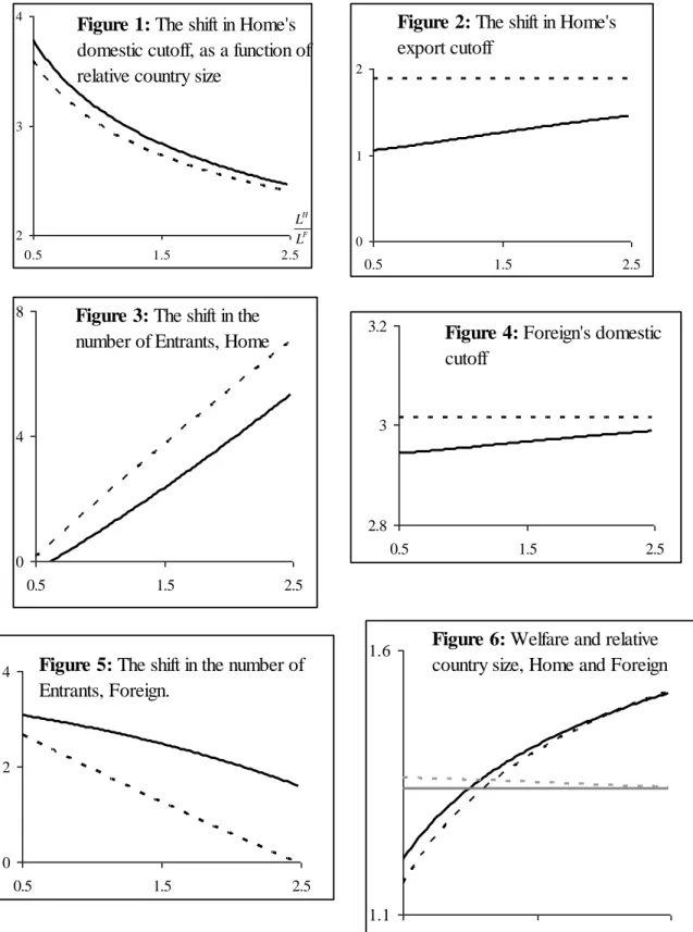
These numerical solutions for (15) and (16) unambiguously show that c increases and DH c DF
decreases in the antidumping scenario. Foreign's AD regime has reduced the attractiveness of setting up a firm in Home, and Foreign is therefore a relatively more attractive place to locate. In the long run, the firms that attempt entry in Foreign will more than replace the displaced imports from Home, and competition will increase. In Home, fewer firms will enter, and eventually competition will start to decrease.8
All long-run implications of Foreign's AD regime are presented below in Result 3 for Home and Result 4 for Foreign. Appendix 2 contains graphs from the simulations, illustrating the results. As with average prices in the previous section, it is possible, but tedious, to express entrants, varieties, price variance and welfare in terms of these new cutoffs. Derivations and expressions may be found in Appendix 1..
8 In Melitz (2003), all firms eventually die out as they are hit by exogenous "bad shocks", and new firms enter to replace
them. This process is not modeled explicitly in Melitz and Ottaviano (2008), but implicitly, all firms have been replaced in the transition from one long-run equilibrium to another. I am thankful to Gianmarco Ottaviano for confirming this.
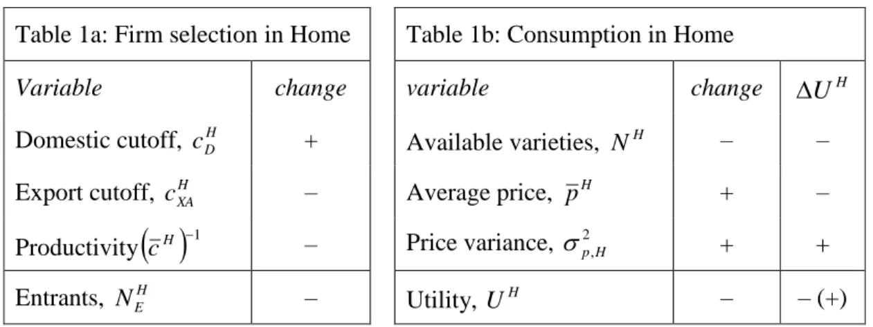
Result 3: Long run effects of a trading partner's antidumping enforcement
Table 1a: Firm selection in Home Table 1b: Consumption in Home
Variable change variable change H
U
Domestic cutoff, c DH + Available varieties, N H – –
Export cutoff, cHXA – Average price, H
p + –
Productivity
cH 1 – Price variance, 2p,H + +Entrants, N EH – Utility, H
U – – (+)
Table 1a summarizes the long-run effects on the composition of firms in Home. Because of its hampered export potential, fewer firms will enter Home, and competition there will therefore decrease: Firms with higher marginal costs can survive, and the average productivity of operating firms therefore falls. Firms must be more productive to become exporters, the effect of the lower export cutoff in (13) is accentuated by tougher competition in Foreign (see below).
Table 1b summarize the effects for consumers in Home, with the UH-column indicating how the change in the variable affects welfare. Lower entry in Home means that consumers there have fewer varieties to choose from. Decreased competition will drive the average price up, in spite of the lower domestic prices set by Home exporters. These lower domestic prices drive the price variance up, however, which enables consumers to substitute towards the varieties that Home exporters sell. On net, however, welfare falls.
It is possible to construct simulations where Home consumers have a small net welfare gain. This may happen if a) Home is very large relative to Foreign, LH >>LF, and b) Home has higher export barriers than Foreign τH>>τF and c) varieties are good substitutes for each other (low γ). Then Home will still have relatively many active exporters to the AD regime, and the positive welfare effects through 2p,Hof lower domestic prices of exported varieties may dominate.
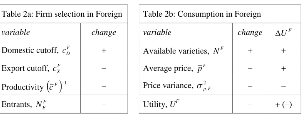
Result 4: Long-run effects in a country enforcing antidumping
Table 2a: Firm selection in Foreign Table 2b: Consumption in Foreign
variable change variable change F
U
Domestic cutoff, c DF + Available varieties, NF + + Export cutoff, c FX – Average price,
F
p – +
Productivity
cF 1 – Price variance, 2p,F – –Entrants, N EF – Utility, U
F –
+ (–)
As summarized in Table 2a, the reduced competition in Foreign due to falling imports attracts new entrants. These new entrants eventually drive competition down below what it was before the AD regime. A firm must have lower marginal costs to survive and average productivity increases. Because of the decreased competition in Home described above, firms in Foreign find exporting easier: The higher export profits raise export sales of existing ex-porters and enable less productive firms to export.
From Table 2b, we see that consumers benefit in Foreign. The new entrants more than compensate for the varieties that are no longer imported from Home, and the increased competition is enough to offset the higher prices of those varieties that are still imported. The price variance, however, decreases because of the fewer and more expensive imports, removing some of the welfare gain. On net, however, consumers benefit.
The negative contribution from reduced price variance may dominate and give a net welfare loss in Foreign, this happens under the same asymmetry conditions that gave Home a welfare gain above: LH >>LF, τH>>τF and low γ.
In short, Foreign's AD protection allows it to "steal firms from Home" and thereby enjoy welfare gains on the expense of Home. These welfare gains are always lower than Home's welfare loss, so there is no room for a compensation scheme between the two countries that leaves everyone better off in the AD regime.9
3 Discussion
The welfare effects of the AD regime presented in results 3 and 4 are similar to what would happen if Foreign unilaterally restricted trade by increasing τF. As Melitz and Ottaviano (2008) show, a country can in the long run enjoy welfare gains from a unilateral trade restriction by attracting firms, again on
9
Results 3 and 4 are qualitatively the same across parameter specifications. Changing technology parameters fE, k and cM or
the demand parameters that govern sector size, α and η, has no quantitative effects, either. As the final paragraphs of results 3 and 4 hint, welfare losses in Home and gains in Foreign are magnified with higher γ, because consumers then care more about variety access and less about price differences. Moreover, the lower trade costs are, the more Foreign's AD policy distort entry patterns, again magnifying the welfare effects.
the expense of its trading partner. The two trade policies are not identical, however: Under the AD regime, Home's welfare losses are softened by the lower domestic prices of Home exporters; if Foreign increases τF, this softening is absent. The simulations confirm that AD gives a "cheaper" welfare in-crease: For a given increase in Foreign's welfare (through either AD or increasing τF), Home suffers a lower welfare loss from AD than from higher τF.
Despite these softer welfare losses from AD, the main message from the analysis of long-run welfare effects is one of concern. Countries have an incentive to unilaterally enforce AD to a degree where it affects firms' location decisions, just as they have an incentive to unilaterally increase their tariffs. The difference is that the WTO allows use of AD.
The situation is akin to a prisoners' dilemma: Foreign's gains from enforcing AD arise only because the AD-protected country becomes relatively more attractive as a location for firms. If Home were to retaliate by also adopting AD legislation and enforcing it credibly, Foreign's welfare gains would disappear, and both countries would lose in comparison to policy regimes without AD. The AD policy equilibrium is inefficient, just like the policy equilibrium for unilateral increases in τl.
Ossa (2011) shows how the GATT/WTO negotiation rules of reciprocity and nondiscrimination (most favored nations) help countries coordinate and escape the prisoner's dilemma outcome for tariff increases. Since AD is sanctioned by the WTO, there is no institutional support to guide countries out of an outcome where countries enforce AD legislation against each other, to the detriment of all.
From this analysis, the recent spread of AD legislation has bleak perspectives. The limited trade-depressing effects of AD that Egger and Nelson (2010) find on aggregate data suggest, however, that we are not in the prisoner's dilemma outcome: The average country does not seem to use AD so intensively that it has noteworthy effect on firm locations. In fact, the current situation of AD use that we observe may be closer to the asymmetric AD scenario described above. Vandenbussche and Zanardi (2010) show that some new adopters of AD (Brazil, India, Mexico, Taiwan and Turkey) use the legislation enough to generate substantial decreases in their imports.
Finally, it is worth summarizing the theoretical gains from modeling AD with heterogeneous firms. Although this paper is the first to point to how a country may gain in the long run from enforcing AD, that particular result can also be derived in a model with homogenous firms. The strength of the framework employed here lies in the ability to expose how effects differ across firms and how export selection and productivity change.
4 Conclusion
This paper has examined the effects of AD in a monopolistic competition model with heterogeneous firms. In the specific policy regime analyzed, AD in one of the two countries is so heavily enforced that firms exporting to the country set prices in a way that avoids any scrutiny by AD authorities. The heterogeneous firms framework provides a series of novel effects of AD:
The direct effects are that exporters in Home (the unprotected country) will either lower their domestic prices to be able to set lower export prices, or they will stop exporting altogether. In the short run, these lower domestic prices hurt Home's non-exporting firms, too, but consumers in Home gain in the short run from the increased competition. In the long run, however, fewer firms will enter Home because of the reduced export potential, and competition will fall. In the long run, the least productive firms gain from this reduced competition, whereas the productive firms still suffer from the reduced export potential. Consumers in Home lose in the long run, competition is lower and there are fewer varieties.
In Foreign, the AD-protected country, competition falls in the short run, because of the reduction in imports. All local firms have higher domestic sales, but exporters lose some export profits because of the lower prices in Home. In the long run, however, new firms will enter Foreign, eventually increasing competition above what is was without AD protection. Foreign's least productive firms therefore have lower profits, whereas exporters gain from decreased competition in Home. Increased competition and more varieties raise the welfare of Foreign's consumers.
These results show how analyzing AD with heterogeneous firms and allowing for long-run industry reallocations may provide new policy insights, and it also raises concerns that countries may use AD policies to enjoy welfare gains on expense of their trading partners.
Appendix 1: Average prices, number of entrants, varieties and welfare
Notation: N and EH F E
N denote the number of firms attempting entry in Home and Foreign, respectively.
They relate to the number of varieties available to consumers in the following manner:
H X H E H D H E H c G N c G N N and NF NEFG
cDF NEHG
cXAH I shall occasionally also use the shorthands ρH = (τH)–k and ρF = (τF)–kAverage prices, Foreign:
Domestic varieties are still priced as
F D F D F D c c c c c p , 0, 2 1 and they make up a fraction NEFG
cDF /NFof the varieties available in Foreign. Imported varieties are in the AD regime priced as
H
XA F H D F H F D H F XA c c c c c c p 1 , 0, 2 1 ,and they make up the fraction NEHG
cXAH /NF of the varieties in Foreign. The average price can therefore be computed from
DF F D c H XA H XA F H XA H E c F D F D F F D F E F A dG c c G c p N c G N c dG c G c p N c G N p 0 0
H
XA H D H H X H F F H XA H E F D F F D F E F A k c c kc k N c G N c k k N c G N p 1 2 2 2 2 1 2Without AD, average prices in Foreign are F cDF k k p 2 2 1 2
, so average prices are higher under AD when
H XA F H D H H X H F F D k c c kc c k1 1 1 2 using that F F D H X c c / , inserting for H XAc and simplifying reveals that this condition is satisfied whenever H
D H
X c
c . As claimed in section 2.6, average prices increase in Foreign. In the long run, cutoffs will change enough to counter this result.
Average prices, Home
Home non-exporters set prices as
H D H D H D c c c c c p , 0, 2 1 . Their varieties make up a fraction
H
H XA H D H E Gc Gc NN / of varieties for sale in Home.
Home exporters set prices as pDH
c
HcXH
1 H
cDH c
, c
0,cHXA
2
1
, and these varieties make up a fraction of the varieties available in Home.
Foreign exporters set prices as pXF
c
cDH Hc
, c
0,cDH /H
2 1 , corresponding to the fraction
DH H
H F E Gc N N / / .The average price can therefore be computed from:
H H D H XA H D H XA c H H D F X H F D F E c H XA H XA H H XA H E c c H XA H D H D H H XA H D F E H A c dG c G c p N c G N c dG c G c p N c G N c dG c G c G c p N c G c G N p / 0 0 /
H XA H X H D H F H E H D H A c c Gc N N c k k p 2 1 2 2 1 2which is lower than the average prices without AD, AH cDH k k p 2 2 1 2
, as claimed in section 2.6. As for Foreign, the result is countered by changed entry in the long run
Number of Entrants
For Foreign, there are two more conditions in the model relating the average price to the number of entrants and varieties, the threshold price condition
DF
F F F D F c p N c N
(from (3)) and the number of active firms, NF NEFG
cDF NEHG
cHXA : Combining these with the average prices gives an expression in N and EF N only. EH
1 1 2 1 1 1 1 1 2 2 2 1 2 k F D F D k M H XA F D F H D F D F H k F D H XA H E F E F D H XA H XA H XA H D H H X H F H E F D F D F E H XA H D H E F D F D F E c c c k kc c c c k c c N N c c G c k k c G c c N c G c k k N c G c N c G c N A similar relation can be computed for Home. Insert average prices into the threshold price condition
H
D H H H D H c p N c N and the number of active firms
DH H
F E H D H E H c G N c G N N / to get:
1 1 2 1 1 1 1 / 2 2 1 2 2 1 2 2 1 2 / k H D H D k M F E H k H D H XA H D F F D H H E H D H H D H D F E H XA H X H D H H E H D H D H E H D H H D F E H D H D H E c c c k N c c c c k N c c G c k k N c G c c N c c G k k N c c G N c c G N Solving for the number of entrants
The number of entrants in Home and Foreign can now be found by solving these two equations for N EF
and N . EH Let
k F D H XA H D F F D H c c c c k A 1 1 1 1 and
H XA F D F H D F D F H k F D H XA c c c c k c c B 1 1 1 1 .Rewrite the two equations as:
1 1 2 k F D F D k M H E F E c c c k B N N and
1 1 2 k H D H D k M F E H H E c c c k N A N Isolating for
N
EF in the upper equation, and inserting into the lower gives:
1 1 1 1 1 2 1 1 2 1 2 k F D F D H k H D H D k M H H E k H D H D k M H E H H E H k F D F D k M c c c c c k B A N c c c k A N B N c c c k The expression is somewhat similar to the expression for entrants derived in Melitz and Ottaviano (2008). Rewriting gives:
1 1 1 1 2 1 k F D F D H k H D H D F H k M H F H H E c c c c c k B A N which is similar to the number of entrants in Melitz and Ottaviano (2008), corrected with H F H B A 1 . Entry distortions not only take place through changes in cutoffs, but also through this term. In all simulations, 1 1 H F H B A
, entry is reduced in Home.
The number of entrants in Foreign:
1
, 2 1 k H D H D k M H E F E c c c k B N N inserting H E N :
1 1 1 1 1 1 1 2 1 2 1 2 k H D H D k F D F D H k M F E k F D F D k M k F D F D H k H D H D k M H F E c c B c c A B A c k N c c c k c c c c c k B A B N Again, there are some similarities to the number of entrants in Melitz and Ottaviano (2008), rewriting to clarify this:
1 1 1 1 1 2 k H D H D F F k F D F D H F H F H k M F E c c B c c A B A c k N Entry into both Home and Foreign are adjusted downwards by the term 1 1 H F H B A . Entry into Foreign is then corrected by A and B, which for all parameters implies an increase, representing how Foreign has become relatively more attractive as a market.
Varieties
With the expressions for the entrants at hand, and numerical solutions for the cutoffs, NH and NF can be found numerically from:
F F
D F E H D H E H c G N c G N N / and NF NEFG
cDF NEHG
cXAHWelfare is given by:
p
N l H F N U pl l l l l , , 2 1 2 1 1 2 2, 1 The price variance is given by 2p,l E
p2 pl2, where p has been derived for each country above. lThe missing term is the second uncentered moment E(p²):
Welfare in Foreign: E[pF(c)²] is given by:
H XA F D H XA F D c k H XA k H D H F F D H F F H XA H E c k F D k F D F F D F E c H XA H XA F H XA H E c F D F D F F D F E F dc c kc c c c N c G N dc c kc c c N c G N c c c dG c p N c G N c c c dG c p N c G N c p E 0 1 2 2 0 1 2 0 2 0 2 2 1 / 4 4 1 | | The integrals give:
F D c F D k F D k F D k k k k c dc c kc c c 0 2 2 1 2 2 1 2 4 1 2 1 4 1 and
H XA H XA F c k H XA k H D H F F D H F c k k M c k k M dc c kc c c c H XA 1 2 2 4 1 / 4 2 2 2 0 1 2 2 , where M HcDF /F
1HcDH
With all these components determined, welfare in Foreign can be computed with numerical values for the cutoffs.
Welfare in Home: E[pH(c)²] is given by: