Changing-regime volatility: A fractionally integrated SETAR model

(1)

HAL Id: halshs-00185369

https://halshs.archives-ouvertes.fr/halshs-00185369

Submitted on 6 Mar 2008

HAL is a multi-disciplinary open access archive for the deposit and dissemination of sci-entific research documents, whether they are pub-lished or not. The documents may come from teaching and research institutions in France or

L’archive ouverte pluridisciplinaire HAL, est destinée au dépôt et à la diffusion de documents scientifiques de niveau recherche, publiés ou non, émanant des établissements d’enseignement et de recherche français ou étrangers, des laboratoires

Changing-regime volatility: A fractionally integrated

SETAR model

Gilles Dufrenot, Dominique Guegan, Anne Peguin-Feissolle

To cite this version:

Gilles Dufrenot, Dominique Guegan, Anne Peguin-Feissolle. Changing-regime volatility: A fractionally integrated SETAR model. Applied Financial Economics, Taylor & Francis (Routledge), 2008, 18 (7), pp.519-526. �10.1080/09603100600993778�. �halshs-00185369�

(2)

Changing-regime volatility: A

fractionally integrated SETAR model

Gilles DUFRENOT

∗

Dominique GUEGAN

†

Anne PEGUIN-FEISSOLLE

‡

January 26, 2006

Abstract

This paper presents a 2-regime SETAR model with diﬀerent long-memory processes in both regimes. We briefly present the long-memory properties of this model and propose an estimation method. Such a process is applied to the absolute and squared returns of five stock in-dices. A comparison with simple FARIMA models is made using some forecastibility criteria. Our empirical results suggest that our model oﬀers an interesting alternative competing framework to describe the persistent dynamics in modeling the returns.

Keywords: SETAR - Long-memory - Stock indices - Forecasting. JEL classification: C32, C51, G12

∗_{ERUDITE, Universit´}_{e Paris 12 and GREQAM, Centre de la Vieille Charit´}_{e, 2 rue de}

la Charit´e, 13002 Marseille, France, Email: Lopaduf@aol.com

†_{Ecole Normale Sup´}_{erieure de Cachan, MORA-IDHE, UMR-CNRS, and Senior}

Aca-demic Fellow de l’IEF, 61 avenue du Pr´esident Wilson, 94235, Cachan, C´edex, France, Email: guegan@ecogest.ens-cachan.fr

‡_{Corresponding author: Anne PEGUIN-FEISSOLLE, GREQAM, Centre de la Vieille}

Charit´e, 2 rue de la Charit´e, 13002 Marseille, France, tel: +33.4.91.14.07.35, fax: +33.4.91.90.02.27, Email: Anne.Peguin@univmed.fr

(3)

1 Introduction

The changing persistence property in the volatility of financial time series has recently emerged in the literature as a new agenda of research. Several approaches have been proposed that include multiple factor models (Gallant, Hsu and Tauchen (1999)), models with transitory and permanent components (Andersen et al. (2003)) and Markov regime switching stochastic volatility models (Hwang, Satchell and Valls (2004). In this paper, we propose a model that extends the SETAR process proposed by Tong and Lim (1980) by introducing a long-memory dynamics. More specifically, we consider a two-regime SETAR model where both two-regimes are characterized by a fractional white noise: ( (1_{− B)}d1_X t = ε (1) t if Xt−1≤ c : regime 1 (1_{− B)}d2_X t = ε(2)t if Xt−1> c : regime 2, (1)

where di ∈ (0, 1/2), i = 1, 2, are fractional diﬀerence parameters, c is a

threshold parameter, ε(i)_t , i = 1, 2, are strong white noises with finite variances and B is the backward shift operator. This model includes the following sub-model as a particular case:

( Xt= ε (1) t if Xt−1 ≤ c : regime 1 (1_{− B)}d_X t= ε (2) t if Xt−1 > c : regime 2, (2)

where the persistent dynamics characterizes one regime only. This sub-model have been studied by Dufrénot, Guégan and Péguin-Feissolle (2005a, 2005b). We extend this previous study by examining whether the mixed evidence of asymmetry and long-memory still holds in a more general case. Models such as (1) and (2) have several advantages over some other existing models recently proposed in the empirical literature. Caporale and Gil-Alana (2004) use the following model:

Xt = f (zt, Θ) + εt, (1− B)dεt = υt, (3)

where f is a nonlinear function (in the variables, not in the parameters), zt is a vector of variables, Θ is a set of unknown parameters and υt is a

white noise process. In their paper, these authors consider a STAR model as their function f . One caveat of their model comes from the fact that nonlinearity and long-memory enter this equation additively. Therefore, one avoids interactions between the parameters of the nonlinear function and the fractional parameter. In our model, the time-varying dynamics of the long-memory parameter is caused by changing regimes (therefore by the value

(4)

of the parameter c). van Djik, Franses and Paap (2002) introduce a model where the values of the nonlinear parameters and the fractional parameter are determined jointly:

(1_{− B)}dXt = " _p X i=1 α1_i(1_{− B)}dX_t−i # F (z_t−l, Θ) + (4) " _p X i=1 α2_i(1_{− B)}dX_t−i # [1_{− F (z}_t−l, Θ)] + εt,

where F is the logistic function, zt is a transition variable and εt is a white

noise process. This can be considered as a nonlinear transformation of a long-memory process. If we assume that z_t−l = X_t−1, p = 1 and

F (z_t−l, Θ) = ½ 1 if z_t−l _{≤ c} 0 otherwise , then (4) is written: Yt= ½ α1 1Yt−1+ εt if Xt−1≤ c α2 1Yt−1+ εt if Xt−1> c , Yt = (1− B)dXt. (5)

This is a SETAR modelling of a fractional white noise. This model has been successfully used to capture the persistent and asymmetric dynamics of the unemployment rate, but it is not convenient for the study of the changing degree of persistence in the volatility of financial time series: indeed, the fractional parameter is assumed to be the same in both regimes. Our model allows more flexibility by considering diﬀerent values of d on diﬀerent states. We consider here the simple case of fractional white noises in each regime.

The paper is organized as follows. Section 2 presents some properties of the model. In Section 3, we present results that successfully match the em-pirical observations of five daily stock indices; we briefly give some economic intuitions to our results. Finally, Section 4 concludes the paper.

2 Some properties of the model, estimation

and prediction

Our definition of long-memory follows Granger (1980): a long-memory be-havior is detected whenever the autocorrelation function of a process shows a slow decrease towards 0. More precisely, we say that a stationary process (Xt)t, with an autocovariance function γX, is long-memory if,∀t and ∀τ,

(5)

where 0 < d < 1/2 and C(d) is a constant which depends only on d. Under the assumption that ε(i)t , i = 1, 2, are strong white noises with finite variances,

model (1) is locally (in each regime) and globally stationary and invertible. Its autocorrelation function, γX(τ ), is written as:

γ_X(τ ) = C(τ , d1)N1(c) + C(τ , d2)N2(c), (7) where, for i = 1, 2, C(τ , di) = Γ(1_{− 2d}i)Γ(τ + di) Γ(di)Γ(1− di)Γ(τ + 1− di) . (8)

N1(c) and N2(c) are the percentages of observations, respectively in regime

1 and in regime 2, and Γ is the Gamma Function. They are not pre-defined, but depends upon the threshold parameter c. The theoretical autocorrelation function is thus a mixture of the autocorrelations of the long-memory models in both regimes. It can be shown, using simulations, that γX(τ ) exhibits a

variety of decay rates (fast to very slow) according to the values of c (see Dufrénot, Guégan and Péguin-Feissolle (2003) for the case where one regime is a short-memory).

Even in a simple formulation such as ours, the estimation of the parame-ters d1, d2and c is more diﬃcult than in the standard case of ARFIMA models

or SETAR models. Ideally, one would like to apply here methods based on maximum likelihood approach (the Whittle estimator), but this is not fea-sible because, as in the standard SETAR model, the log-likelihood function is not continuously differentiable with respect to the threshold parameters. In the standard SETAR modeling, the estimation methods are generally se-quential (see Tong (1990), Tsay (1989) or Hansen (1997 and 2000) among others); nevertheless, some recent papers try to develop different methods in order to make a joint estimation of the parameters (by using some factoriza-tions as in Coakley, Fuertes and Pérez (2003), Bayesian method as in So and Chen ( 2003) or genetic algorithm as in Wu and Chang (2002)). The trans-position of these methods to our case is, however, not feasible because of the presence of the fractional parameters in the regimes. We can neither apply the estimation procedure proposed for nonlinear long-memory model such as in van Dijk, Franses and Paap (2002)’s model because of the discontinuity of the two regimes characterizing the model given by (1). The approach we adopt here is very similar in spirit to the methodology suggested by Tsay (1989). This amounts to a) determine a plausible value for the threshold parameter1_{, and b) estimate the other parameters of the model conditionally}

(6)

on this threshold value (see Dufrénot, Guégan and Péguin-Feissolle (2005a and 2005b)).

Estimation of the long-memory SETAR model

The diﬀerent steps used to estimate the model are thus the following: • Estimate the value of the threshold parameter c (the procedure is

de-scribed below).

• Separate the observations in two sub-groups according to the estimated value of c and deduce N1(c), N2(c).

• For each sub-group, estimate the fractional parameter. The estima-tion of the fracestima-tional parameters is based on the GPH log-periodogram approach, initially proposed by Geweke and Porter-Hudak (1983) and refined by Robinson (1995). More precisely, in the general case of a long-memory parameter d, we denote I(ωj) the sample periodogram at

the jth _{Fourier frequency, where ω}

j = 2πj/T , j = 1, 2, ..., [T /2]. The

fractional parameter is based on the following regression:

log [I(ωj)] = a + b log(ωj) + εj, (9)

where j = 1, ..., m and bd = _{−bb/2. The t-ratios are computed using} both the estimated and the theoretical standard errors π(24m)−1/2_(we

choose m = T0.8 and use all of the first Fourier frequencies.

Locating the threshold parameter

A crucial point concerns the step where the parameter c has to be es-timated. We first construct the time series ( eXt)t of arranged observations

according to the decreasing values of X_t−1 and then proceed as follows: 1. One considers a set of s1 initial observations of ( eXt)t and estimate the

long-memory parameter and the corresponding t_{− ratio: t}s1.

2. The vector ( eXt)t is then incremented in such a way to contain s2, s3,

..., sn observations; new long-memory parameters and their t− ratios

are computed: ts2, ts3,... , tsn (in the applications, we add one

obser-vation: sj = sj−1+ 1 for all j).

standard short-memory SETAR models. Because of the presence of a long-memory regime, the method used here to locate the threshold parameter is diﬀerent and is explained in the following paragraphs.

(7)

3. Consider the set of estimated t-ratios _{ts1, ts2, ts3, ..., tsn}. One tests

for the presence of a structural break et in the sequence of t-ratios. A simple way to do this is to use a standard Chow test. The series of t-ratios is regressed on a linear time trend, using incremented dummy variables: for t = 1, 2, . . . , n

ts_t = (α + βDt) + (γ + δDt)t + ut, (10)

where ut is a sequence of iid random variables and

Dt=

½

1 if t_{≤ et} 0 otherwise.

We test the null hypothesis H0 : β = δ = 0 against the alternative

β _{6= 0 or γ 6= 0. The constant term is omitted if we only want to} test changes in the slope. The test is implemented by considering dif-ferent values of et and finally one retains the value yielding the lowest p-value. Instead of using the Chow test, one can also compute the sum of squared residuals corresponding to the equation and select the t-ratio (and thus the threshold value) yielding the lowest sum.

Forecasts for a SETAR model

To make forecast with a SETAR model stays until now an open problem. Some works have been done in a Gaussian context. Here, we assume that the observations are explained by a process such that (1). Say, we assume that (Xt)tis a linear autoregression within a regime, but may move between

regimes depending on the values taken by a lag of Xt, say Xt−1. Then, in

each regime, (Xt)t can be rewritten as:

(I_{− B)}di_X t = εt (11) or Xt= diXt−1+ di(1− di) 2 Xt−2+ ... + di(1− di)...(k− di− 1) k! Xt−k+ ... + εt

with i = 1, 2. Then we write the model (11) as:

Xt= ∞

X

k=1

(8)

with

πi,k=

Γ (k_{− d}i)

Γ (k + 1) Γ (_−di)

.

Assume now that we observe (X1,· · · , Xn) and denote In the σ−algebra

generated by (Xs, s ≤ n). We will denote respectively by I1,n and I2,n the

σ_{−algebra generated by the observations which belong to the regime one or} to the regime two. At time n, for an horizon k, the forecasts are respectively equal to (using equation (12)):

b X1,n+k = E [Xn+k|I1,n] = ∞ X j=1 π1,jXb1,n+k−j, (13)

for regime 1 and

b X2,n+k = E [Xn+k|I2,n] = ∞ X j=1 π2,jXb2,n+k−j, (14)

for regime 2. Then, the forecast ˆXn+k is given by:

ˆ

Xn+k = ˆX1,n+k+ ˆX2,n+k, (15)

for k = 2,_{· · · . We remark in equations (13) and (14) that we need to use an} infinite sum, and in practice we will truncate this sum for a large N. Thus we get an ”approximation” of the true forecast.

3 Application to absolute and squared returns

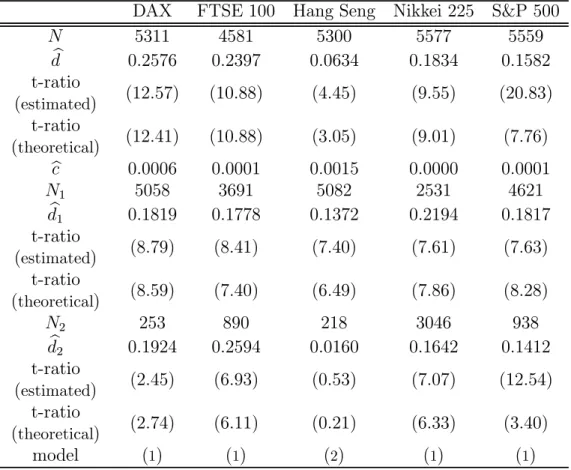
To see how the model matches the empirical data, we consider the absolute and squared returns of five daily stocks indices over the period 01/04/1981 to 01/18/2002: DAX, FSTE 100, Hang Seng, Nikkei 225 and S&P 500. These data were used by Bhardwaj and Swanson (2005), who applied ARFIMA models to the series and found that the latter frequently outperform lin-ear models in terms of prediction. In their paper, the authors suggested, as an interesting extension to their work, to see whether nonlinear models with regime-switching or thresholds would perform better than the ARFIMA models. We consider the two-regime SETAR model as an alternative to the ARFIMA model. Tables 1 and 2 report the estimates for respectively the ab-solute and squared returns on the whole period. As observed, we successfully detect diﬀerent orders of fractional integration in each regime, for a majority

(9)

of cases. In one case (Hang Seng in table 2), we retrieve the sub-model (2) with a white noise dynamics in one regime. We also find evidence of a pos-sible dynamics with a nonstationary long-memory dynamics in one regime (absolute returns for the FTSE 100).

The finding of regimes of volatility with different orders of integration is in line with several economic findings in the behavioural finance literature. A first possible explanation lies in the interacting behaviour of a diversity of agents in the financial markets. Multi-agent microeconomic models, with interactions between noise traders and fundamentalists and showing a ”herd-ing mechanism”, have been proposed in the literature, that are capable of reproducing statistical properties in accordance with the empirical finding of changing volatility and long-memory (see, Lux and Marchesi (2000), Kir-man and Teyssière (2002), Iori (2002), Alfarano and Lux (2002)). What these models suggest is that changing strategy configurations (whether or not the market is dominated by a given category of agents) generate changes in both the burst of activity (thereby implying variations in the volatility) and in the degree of friction of the markets (frictions explain the presence of long-memory in volatility). A second justification to the evidence of a joint switching and long-memory dynamics in the absolute and squared re-turns may be the presence of multiple attractors in volatility clustering, with occasional or recurrent switches between these attractors. In our case, the at-tractors are characterized by different states with specific degree of volatility and long-memory. Such a phenomenon is viewed as a sign of ”intermittency” in volatility clustering (for an illustration, see Gaunersdorfer, Hommes and Wagener (2001)).

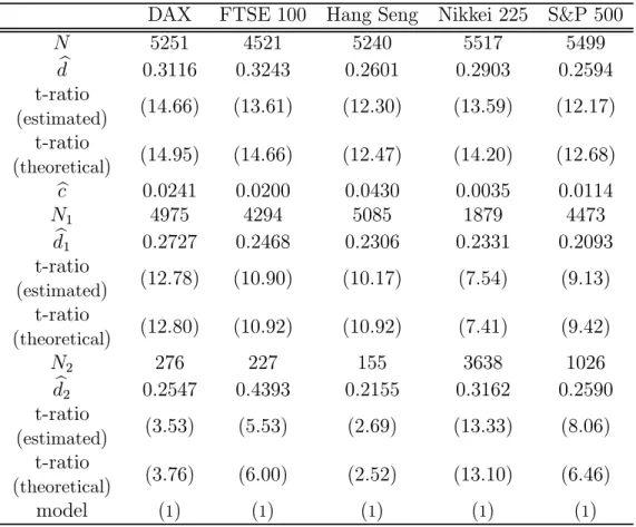
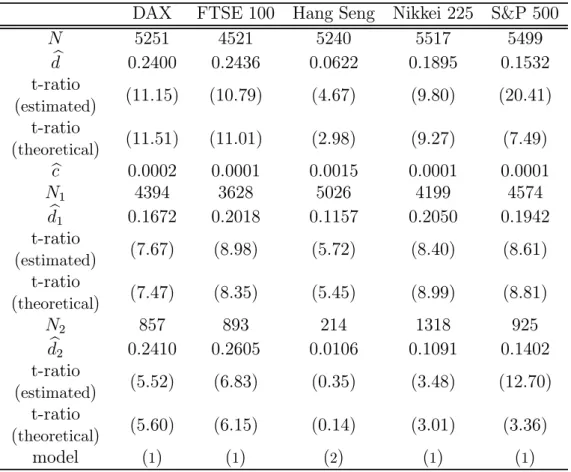
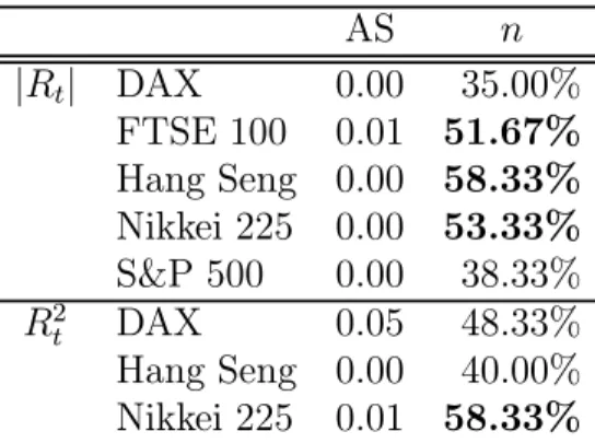
We use the model to compute out-of-sample dynamic predictions on the last three months (60 observations) and evaluate the prediction accuracy us-ing the asymptotic test defined in Diebold and Mariano (1995). Therefore, we estimate our SETAR long-memory model and an ARFIMA model on a shorter period: the whole period excluding the last three months. We give in tables 3 and 4 the new estimation results: they are not fundamentally differ-ent from the results on the whole period, except in the case of the Nikkei 225 where the regimes are very different, showing an instability of the behavior of the absolute and squared returns of this series. In table 5, we report the p-values of the test of predictive accuracy of our model versus an ARFIMA model. We give only the cases where there exists a significant difference of the predictive accuracy for the different models; in the other cases, the mod-els do not give significantly different prediction performance. Therefore, the numbers in bold correspond to the cases where the predictions of the SETAR long-memory model are better than those of a ARFIMA model: the number n indicates the percentage of points for which the residuals of our model

(10)

are inferior to those of the standard long memory model. As observed, the two-regime SETAR model outperforms the ARFIMA model in 40% of the cases (see the cases where n is higher than 50%).

4 Conclusion

This paper has proposed a threshold model that accounts for both the regime-switching and long-memory dynamics of volatility. Our approach introduces a fractional component in a two-regime SETAR model. The model matches the empirical data and reveals the presence of two distinct long-memory regimes in the volatility of five stock indices. The results are in line with some economic intuitions provided by the literature on behavioural finance. We envisage two extensions to the paper. Firstly, it would be interesting to compare the performance of two types of regime-switching long-memory models: a model where the changing dynamics is described by a Markov switching process and another by a SETAR model. As one knows, a key difference between these processes comes from the nature of the switching process (stochastic in the case of Markov switching models and determin-istic in the case of the threshold models). Whether or not the nature of the switching dynamics affects the long-memory dynamics is an interesting question. Secondly, the model can be applied directly to GARCH family processes, for instance by estimating a two-regime FI-GARCH model with different fractional parameters.

(11)

References

[1] Alfarano, S. and T. Lux (2002) A minimal noise traders model with realistic time series properties, Symposium of the Society of Nonlinear Dynamics and Econometrics, Atlanta, March.

[2] Andersen, T.G., J. Bollerslev, F.X. Diebold and P. Labys (2003) Mod-elling and forecasting realized volatility, Econometrica, 71, 579-625. [3] Bhardwaj G. and N.R. Swanson (2005) An empirical investigation of the

usefulness of ARFIMA models for predicting macroeconomic an financial time series, Journal of Econometrics, forthcoming.

[4] Caporale, G.M. and L.A. Gil-Alana (2004) Nonlinearities and fractional integration in the US unemployment rate, Discussion paper, Hamburg Institute of International Economics.

[5] Coakley, J., A.M. Fuertes and M.T. P´erez (2003) Numerical issues in threshold autoregressive modeling of time series, Journal of Economic Dynamics and Control, 27, 2219-2242.

[6] Diebold, F. X. and R. Mariano (1995) Comparing predictive accuracy, Journal of Business and Economic Statistics, 13, 3, 253-263.

[7] Dufrénot, G., D. Guégan and A. Péguin-Feissolle (2003) A SETAR model with long-memory property, International Conference on Fore-casting Financial Markets, Paris, June.

[8] Dufrénot, G., D. Guégan and A. Péguin-Feissolle (2005a) Modelling squared returns using a SETAR model with long memory dynamics, Economics Letters, 86, 2, 237-243.

[9] Dufrénot, G., D. Guégan and A. Péguin-Feissolle (2005b) Long-memory dynamics in a SETAR model - Applications to stock markets, the Jour-nal of InternatioJour-nal Financial Markets, Institutions & Money, 15, 5, 391-406.

[10] Gallant, H.R., C. Hsu and G. Tauchen (1999) Using the daily range data to calibrate volatility diﬀusions and extract the forward integrated variance, Review of Economics and Statistics, 81, 4, 617-631.

[11] Gaunersdorfer, A., C. Hommes and F. Wagener (2001) Adaptative be-liefs and the volatility of asset prices, Center for Nonlinear Dynamics in Economics and Finance, University of Amsterdam.

(12)

[12] Geweke, J. and S. Porter-Hudak (1983) The estimation and application of long-memory time series models, Journal of Time Series Analysis, 4, 221-238.

[13] Granger, C.W.J. (1980) Long memory relationships and the aggregation of dynamic models, Journal of Econometrics, 14, 227-238.

[14] Hansen, B.E. (1997) Inference in TAR models, Studies in Nonlinear Dynamics and Econometrics, 2, 1-14.

[15] Hansen, B.E. (2000) Sample splitting and threshold estimation, Econo-metrica, 68, 3, 575-603.

[16] Hwang, S., S. Satchell and P. Valls (2004) How persistent is volatility? An answer with Markov switching stochastic volatility models, Working paper, Cass Business School, Faculty of Finance, London.

[17] Iori, G. (2002) A micro-simulation traders’ activity in the stock market: the rule of heterogeneity, agents’ interactions and trade friction, Journal of Economic Behaviour and Organization, 49, 269-285.

[18] Kirman, A. and G. Teyssi`ere (2002) Microeconomic models of long-memory in the volatility of financial time series, Studies in Nonlinear Dynamics and Econometrics, 4, 1083-1123.

[19] Lux, T. and M. Marchesi (2000) Volatility clustering in financial mar-kets: a micro-simulation of interacting agents, International Journal of Theoretical and Applied Finance, 3, 667-702.

[20] Robinson, P.M. (1995) Log-periodogram regression of time series with long-range dependence, Annals of Statistics, 23, 1048-1072.

[21] So, M.K.P. and C.W.S. Chen (2003) Subset threshold autoregression, Journal of Forecasting, 22, 49-66.

[22] Tong, H. (1990) Non-linear time series - a dynamical systems approach, Oxford University Press.

[23] Tong, H. and K.S. Lim (1980) Threshold autoregressions, limit cycles, and data, Journal of the Royal Statistical Society B, 42, 245-292 with discussions.

[24] Tsay, R.S. (1989) Testing and modelling threshold autoregressive pro-cesses, Journal of the American Statistical Association, 84, 231-240.

(13)

[25] van Dijk, D., P. H. Franses and R. Paap (2002) A nonlinear long-memory model with an application to US unemployment, Journal of Economet-rics, 110, 135-165.

[26] Wu, B. and C.L. Chang (2002) Using genetic algorithms to parame-ters (d,s) estimation for threshold autoregressive models, Computational Statistics and Data Analysis, 38, 315-330.

(14)

Table 1. Estimation of parameters for _|Rt|

on the whole period

DAX FTSE 100 Hang Seng Nikkei 225 S&P 500 N 5311 4581 5300 5577 5559 b d 0.3134 0.3281 0.2552 0.2887 0.2508 t-ratio (estimated) (15.61) (14.72) (12.08) (14.16) (12.04) t-ratio (theoretical) (15.10) (14.90) (12.28) (14.18) (12.31) bc 0.0239 0.0206 0.0400 0.0119 0.0126 N1 5019 4367 5100 4300 4688 b d1 0.2499 0.2313 0.2215 0.2914 0.1979 t-ratio (estimated) (11.44) (9.16) (9.81) (12.38) (9.18) t-ratio (theoretical) (11.77) (10.30) (10.50) (12.90) (9.07) N2 292 214 200 1277 871 b d2 0.1900 0.5167 0.1775 0.2010 0.2865 t-ratio (estimated) (2.88) (6.06) (1.93) (5.34) (7.07) t-ratio (theoretical) (2.86) (6.89) (2.30) (5.47) (6.70) model (1) (1) (1) (1) (1)

Note: The change point in the t-ratios was obtained using the method based on the Chow test. All the estimations are made with GPH method. dbrefers to the estimated fractional parameter andN to the number of observations of the whole sample;db1 anddb2

refer to the estimated fractional parameter and N1 and N2 the number of observations,

respectively in regime 1 and regime 2. The t-ratio must be compared 1.96 (corresponding to the critical value at the 5% level of significance); a non-significant parameter indicates that the volatility is driven by a white noise process (and is thus unpredictable). Con-versely, a significant parameter means that the volatility exhibit a long-memory dynamics therefore yielding to a high predictability. The row ”model” shows the corresponding adequate model (1) or (2).

(15)

Table 2. Estimation of parameters for R2 t

on the whole period

(16)

Table 3. Estimation of parameters for _|Rt| on the whole

period excluding the last three months

(17)

Table 4. Estimation of parameters for R2

t on the whole

period excluding the last three months

(18)

Table 5. Test of predictive accuracy:

our model versus an ARFIMA model (p-values) AS n |Rt| DAX 0.00 35.00% FTSE 100 0.01 51.67% Hang Seng 0.00 58.33% Nikkei 225 0.00 53.33% S&P 500 0.00 38.33% R2 t DAX 0.05 48.33% Hang Seng 0.00 40.00% Nikkei 225 0.01 58.33%

Note: AS is the p-value of the asymptotic test of Diebold and Mariano (1995) and

nis the number of times in percent where the residuals coming from the SETAR model with long memory regimes are smaller than the residuals coming from a standard long memory model (when n>50%, it means that the SETAR model seems the best). The null hypothesis is the hypothesis of equal accuracy of diﬀerent predictive methods. The loss function is quadratic. The test statistics follows asymptotically a N (0, 1) and the truncation lag is 10.