HAL Id: hal-01919788
https://hal.archives-ouvertes.fr/hal-01919788
Submitted on 12 Nov 2018
HAL is a multi-disciplinary open access
archive for the deposit and dissemination of
sci-entific research documents, whether they are
pub-lished or not. The documents may come from
teaching and research institutions in France or
abroad, or from public or private research centers.
L’archive ouverte pluridisciplinaire HAL, est
destinée au dépôt et à la diffusion de documents
scientifiques de niveau recherche, publiés ou non,
émanant des établissements d’enseignement et de
recherche français ou étrangers, des laboratoires
publics ou privés.
Joining multi-epoch archival aerial images in a single
SfM block allows 3-D change detection with almost
exclusively image information
Denis Feurer, F. Vinatier
To cite this version:
Denis Feurer, F. Vinatier. Joining multi-epoch archival aerial images in a single SfM block allows 3-D
change detection with almost exclusively image information. ISPRS Journal of Photogrammetry and
Remote Sensing, Elsevier, 2018, 146, pp.495 - 506. �10.1016/j.isprsjprs.2018.10.016�. �hal-01919788�
The Time-SIFT method : detecting 3-D change from archival photogrammetric analysis with almost exclusively image information
Joining multi-epoch archival aerial images in a single SfM block allows 3-D
change detection with almost exclusively image information
D. Feurera,∗, F. Vinatiera
aLISAH, Univ Montpellier, INRA, IRD, Montpellier SupAgro, Montpellier, France
Abstract
Archival aerial imagery is a worldwide resource for documenting past 3-D change at very high-resolution. However, external information is normally required so that accurate 3-D models can be computed from archival aerial imagery. In this research, we propose and test a new method which joins multi-epoch images in a single block in the first steps of the SfM processing. It allows for computing coherent multi-temporal digital elevation models (DEMs) using just image information. This method is based on the invariance properties of the feature detection procedures that are at the root of the structure from motion (SfM) algorithms.
On a test site covering 170 km2, we applied SfM algorithms to a single image block consisting of all images captured at four
different epochs and spanning a forty year period. We compared this approach to the more classical methods which imply a separation of epochs in different processing blocks. We tested different densities of ground control points derived simply and cheaply from a recent orthophoto and DEM, different ways of image preprocessing and different autocalibration procedures. By determining which choice most affected the final result through this extensive testing procedure, we evaluated the potential of the proposed method for detecting 3-D change.
Our study showed that the proposed method resolves the problem of registration between epochs, so allowing the production of informative DEMs of difference using almost exclusively image information and limited photogrammetric expertise and human intervention. As the proposed method can be automatically applied using just image information, our results pave the way to more systematic processing of archival aerial imagery with very large spatio-temporal windows, which should greatly help document of past 3-D change.
Keywords: Automation, Multitemporal DEMs, SfM Photogrammetry, Analog imagery, 3-D Change Detection, Cost-effective / Frugal
1. INTRODUCTION
For decades, aerial imagery has been used to produce large-scale geographic and topographic maps. Most often with sub-metric reso-lutions, archival aerial imagery has a remarkable coverage in both the temporal and spatial dimensions. Archival aerial imagery has existed in almost every country in the world since the first half of the twentieth century (Cowley and Stichelbaut,2012). This imagery was most often acquired with stereoscopic coverage, which results in a unequalled po-tential for 3-D documentation of past changes. In addition, during the past decade, 3-D past change have been studied using archival aerial imagery in the disciplines of archaeology (Verhoeven,2011;Sevara,
2013;Verhoeven and Vermeulen,2016;Salach,2017;Sevara et al.,
2017), geomorphology (Gomez et al.,2015;Gonc¸alves,2016; Ishig-uro et al.,2016;Bakker and Lane, 2017), glaciology (Mertes et al.,
2017;M¨olg and Bolch, 2017;Vargo et al., 2017), and volcanology (Gomez,2014).
However, the full potential of this very large volume of historical data might have not been widely exploited yet. This circumstance is mainly because accurate processing of historical aerial imagery time series for 3-D change assessment requires other information beyond the images themselves. Indeed, external information such as camera
∗Corresponding author
Email address:denis.feurer@ird.fr (D. Feurer)
calibration certificates, ground control points (GCPs), or the a priori knowledge of stable zones is needed to estimate exterior and interior orientation of the image blocks. This aspect is even more important when the aim is to compute digital elevation models (DEMs) of dif-ferences (abbreviated as DoD byLane et al.(2003);Wheaton et al.
(2010);Williams(2012)), which require that differentiated DEMs are both accurate and spatially consistent in comparison with one another. Historically, the construction of 3-D models began with photogram-metry, first with stereoscopic analysis of oriented image pairs and then with automatic correlation of oriented images (see for exampleKraus and Waldh¨ausl,1998). Using these ’classical’ photogrammetric meth-ods, there are several examples of authors succeeding in differencing DEMs within the most favourable conditions, i.e., when the image datasets were associated with all of the necessary calibration certifi-cates (Fabris and Pesci,2005;Fischer et al.,2011;Micheletti et al.,
2015;Aucelli et al.,2016;Fieber et al.,2018). Having calibration cer-tificates is not sufficient, however.Fischer et al.(2011) andFieber et al.
(2018) - in a specific case that implied DoD with a satellite DEM for the latter work - needed to proceed with additional co-registration of the photogrammetric DEMs, with a priori knowledge and manual de-limitation of stable areas when necessary. Moreover, the use of ’clas-sical’ photogrammetric software, requires accurate initial information (interior orientation, ground control points) to enable the processing to succeed. For example, in work realised with the ERDAS LPS
soft-ware, Micheletti et al. (2015) had to give a specific care to ground control point choices, positioning, distributions and accuracies.
When calibration certificates are missing, which is not rare for the oldest images, interior geometry can be estimated through autocalibra-tion, which estimates simultaneously the interior and exterior orienta-tions. This method was successfully used by several authors with the approach of computing DoDs thereafter (e.g.Chandler and Cooper,
1989;Walstra et al.,2007;Redweik et al.,2016). In their pioneering work,Chandler and Cooper(1989) reminded that the interior orienta-tion consists of two groups of parameters: the parameters that char-acterise the displacement of the principal point relative to the fiducial marks and the parameters that characterise the lens distortion. To these parameters, it is necessary to add the deformation due to the scanning, which has a strong impact on the performance of the 3-D estimation (Sevara,2016). These additional unknowns severely increase the need for ground control points, which in turn raises new issues : the need for expensive additional ground survey and the problem of the accuracy of the orientation estimation with self-calibration algorithms (Aguilar et al.,2013).
A frequent strategy for collecting these additional GCPs at a limited cost is to rely on recent data. These are usually of better quality and are associated with existing and accurate calibration information, fidu-cial marks and/or even contemporary GCPs. James et al.(2006) ex-tracted different numbers of required GCPs from a shaded-view of a li-dar DEM and then detected 3-D change from photogrammetric DEMs estimated with older images. Several authors exploited a well-known or well-established geometry of recent image blocks: they extracted GCPs from these recent images and used these GCPs in older imagery to determine the interior and exterior orientation of these older image blocks (Hapke,2005;Dewitte et al.,2008;Zanutta et al.,2006;Fox and Cziferszky,2008).Nagarajan and Schenk(2016) noticed that success-ful 3-D change detection relies on the use of adequate GCPs, but that collection of these is often too expensive and too cumbersome. They hence proposed a method for co-registrating images on the basis of stable linear features. More recently,Giordano et al.(2018) proposed a method that allows for an automatic collection of these GCPs. GCPs are detected in a recent orthophoto and DEM and then are transferred to images of previous epochs. The method relies on the detection of keypoints between images of different epochs, which is made possible through a first estimation of coarse DEMs and orthophotos of ancient epochs. These first estimates are performed on the basis of the avail-able image metadata at all of the epochs.
The advent of structure from motion (SfM) and multi-view stereo (MVS) algorithms in geoscience and archaeology over the past decade have provided a new paradigm. Indeed, as explained for example by
Westoby et al.(2012) orFonstad et al.(2013), SfM algorithms com-pute relative orientations with only image information, due to key-point detection algorithms such as the scale invariant feature transform (SIFT) (Lowe,2004). The potential of SfM-MVS algorithms for 3-D exploitation of archival aerial imagery was detected very early by Ver-hoeven(2011) who succeeded in obtaining a visual 3-D model from historical aerial imagery with exclusively image information. More-over, the use of SfM software usually does not require advanced skills in photogrammetry, which has allowed a wider use of these techniques, as noted in recent reviews (Eltner et al.,2016;Smith et al.,2016; Mos-brucker et al.,2017). However, even if SfM algorithms have allowed for a more accessible and more straightforward use of archival aerial imagery, this finding did not eliminate the need for thorough control of image acquisition geometry for differencing the DEMs computed with such imagery. Bakker and Lane(2017) noted that SfM-MVS pho-togrammetric processing shares the limitations of classical methods : the propagation of linear errors into the final DEMs requires specific
correction procedures for subsequent accurate DEM differencing. Once again, the control of image and DEM geometry in SfM-based workflows was accomplished through the use of additional external in-formation. Several authors have used GCPs to help the autocalibration (Gomez,2014;Verhoeven and Vermeulen,2016;Mertes et al.,2017).
Cogliati et al.(2017) relied on vector data for co-registration. Due to high residuals on the GCPs, they used a small amount of GCPs for a first estimate of orthophotos and DEMs at each epoch. The hori-zontal georeferencing was then refined with an external 1:5000 vector map, finally allowing for the computation of the height differences. Finally, most authors have directly co-registered the individual DEMs obtained from archival aerial imagery onto reference DEMs, with an a priori knowledge of stable zones (Bakker and Lane,2017;Mertes et al.,2017;M¨olg and Bolch,2017;Sevara et al.,2017).
Finally, as remarked for example byJames et al.(2017) in the con-text of unmanned aerial vehicle imagery processing, it is worthwhile to note that the quality and consistency of surveys realised with SfM-MVS algorithms still rely on an in-depth adjustment of the processing parameters. Parameter adjustments can be even more complex and sensitive when addressing the interior orientation of archival aerial im-agery due to the additional degrees of freedom. Moreover, the acqui-sition geometry of historical aerial datasets does not meet the require-ments of SfM algorithms. First, the former are classically performed with 60% longitudinal and 20% lateral overlaps when the latter require overlaps that exceed 80% longitudinally and 60% laterally. Second, constant and large flying heights - relatively to terrain steepness - con-stitute difficult cases for autocalibration, particularly when based on image information only. Thus, and even if SfM-MVS algorithms had made 3-D exploitation of aerial imagery more widely accessible, the processing of archival imagery has still required manual intervention to avoid gross errors. This goal has been accomplished by visual in-spection throughout all of the processing (e.g.Bakker and Lane,2017) or with complex strategies for the choice of parameters (e.g.Verhoeven and Vermeulen,2016).
Thus, even if SfM photogrammetry could allow a broader use of historical aerial imagery, all of the existing methods for extracting 3-D change from this archive still rely on external data, significant expertise and/or parameter optimisations. This need for expertise and additional data still impedes the actual unlocking of large archival aerial imagery datasets. There is hence a need for a method that would allow the auto-mated production of DoDs from archival aerial imagery with minimal external data and expertise.
In this context, our study aims to assess a new method that bene-fits from the SIFT-like algorithm capabilities for a new purpose. The invariance of features detected by SIFT-like algorithms is originally spatial. It consists in invariance to scale and to simple geometric trans-forms. Our work relies on the fact that SIFT-like algorithms also show invariance over time, as noted for example byChanut et al.(2017), and byVargo et al.(2017). The principle of our proposed method is to merge all of the epochs of a collection of historical image archives in the same SfM processing. Our work proposes and tests an automatic method in which images from different epochs are processed all to-gether in the same block during the SfM step, which is only split then for the DEM estimation step. As a result, all DEMs share by construc-tion a same unique geometric reference, which saves the expensive and/or cumbersome collection of additional external data. Moreover, placing all images in the same block may diminish the linkage between the interior end exterior orientation unknowns. To that end, process-ing parameters can be set so that SfM processprocess-ing of images of differ-ent epochs in the same unique block would take into account the fact that (i) interior orientation of images taken with the same camera are the same, and that (ii) interior orientation of images taken at
differ-ent epochs (and hence with differdiffer-ent cameras) have differdiffer-ent interior orientation parameters. The proposed method would hence allow the use of SfM algorithms on multi-temporal data sets with very few pho-togrammetric expertise and avoiding complex strategies for the tuning of processing parameters.
To the best of our knowledge, there is no existing study which quantitatively and qualitatively assessed the potential of a method that would systematically gather images of different epochs in the first steps of SfM algorithms for DEM differencing. The aim of our paper is hence to assess the potential of the proposed method to automatically obtain informative DoDs with limited input from the user, i.e., with almost no information other than image information and with limited expertise in photogrammetric processing.
In this paper, we propose a test of the different classical process-ing methods that are usually used in the literature compared with the proposed method. 3-D models and DoDs are computed with different processing options and their quality is then assessed with independent DEMs. This analysis allows us to determine the most significant pro-cessing options. A visual inspection of specific 3-D change detected in the DoDs is also performed to ascertain the capacity of the proposed method for mapping past 3-D change.
2. Materials and methods
2.1. Test site and image data
The test site is a 170 km2 rectangle of a Mediterranean landscape
located in Occitanie in southern France (43◦5N, 3◦19E). This zone is
mainly covered by vineyards with forests in its uppermost areas. This zone exhibited a change in land management through a severe trans-formation of vineyard areas during the 1980s, from goblet to trellised vineyards, with a progressive land abandonment and urbanisation over the past 50 years (Vinatier and Arnaiz,2018). The altitudes vary be-tween 0 and 350 m (Figure1). Since 2008 the IGN, the French Na-tional Geographic Institute, started a vast digitisation program. They scanned original archival films with photogrammetric-grade scanners. This archive was recently released and is freely available on the IGN’s website (https://remonterletemps.ign.fr/). The fact that these images were scanned with photogrammetric scanners is important for further photogrammetric processing as noted bySevara(2016) and ob-served in a preliminary study (Feurer et al.,2017). We downloaded a sample of these data at four different epochs allowing for a stereo coverage of the entire test site (coloured polygons on Figure1). The characteristics of these images are reported in Table1.
2.2. Investigated processing options
We aimed at assessing the interest of the proposed method relatively to other existing - and affordable - processing strategies. We hence tested four groups of processing options that would occur at various steps of the SfM-MVS processing chain. The SfM-MVS chain used was AgiSoft Photoscan Pro c. In order to allow for the multi-factorial
analysis of the results of the different processing options tested, the processing parameters of the SfM-MVS processing chain were fixed (see section2.3for the detail of the SfM-MVS processing). The four groups of tested processing options are independent and are described in the four sub-sections below. In order to determine the impact of each group of processing options - including the new method of join-ing multi-epoch images in a sjoin-ingle block - all the combinations, i.e. all possible processing scenarios, were tested. The four groups of process-ing options were: (i) pre-processprocess-ing options, (ii) use of a multi-epoch block, (iii) use of additional manually marked points and (iv) autocal-ibration. The combinations between each different options of the four groups of options resulted in 36 different scenarios, which were all
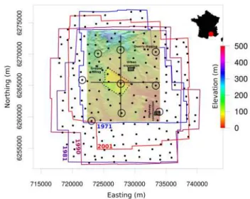
Figure 1: Localisation of the test area, image data, external DEMs and addi-tional points. The coarse DEM used for validation, represented in colour scale, covers the whole test area of 170 km2. The smaller area bordered by dashed
lines corresponds to the second validation DEM, represented with the same colour scale. Black points represent the 200 manually marked points. Points belonging to the minimal set of 9 manually marked points are circled. Shaded rectangles highlight the zones where full resolution qualitative analysis of the DoDs was done. Two perpendicular lines correspond to the North-South and East-West transects. Approximate footprints of the image blocks are repre-sented by coloured polygons. Map projection : Lambert 93 (EPSG:2154)
tested. With 4 different epochs, it resulted in 144 different DEMs and 108 DoDs.
2.2.1. Image pre-processing
Converting image coordinates into camera coordinates requires con-sideration of (i) the film movement in the camera body between two image acquisitions (ii) possible film deformations during storage and (iii) possible geometric deformations during the film scanning. Fidu-cial marks are usually used to estimate the geometric transform be-tween the image coordinates and camera coordinates. Another point, which was raised byGomez et al.(2015) and questioned byBakker and Lane(2017), is the fact that the image borders, where fiducial marks and other metadata appear, can interfere with the automated feature detection algorithm used in SfM workflows and could need to be masked.
Three options were hence tested. The first option, namely the
orig-inal, consisted in using images ’as is’, i.e. without any pre-processing. The second option, namely cropped, consisted of a simple image crop in such a way that the image borders were removed. The third option, namely ReSampFid, consisted of a resampling of the scanned images based on the four fiducial marks of the corners in such a way that the resulting images shared the same geometry, with fiducial marks centres constituting the corners of the resampled images. Even if recent ver-sions of AgiSoft Photoscan Pro c allow the handling and now, for the
most recent versions, the automated detection of fiducial marks, this functionality is not yet effective for older fiducial marks - in our case images before 1981. The third option was hence performed with the ReSampFid tool of the MicMac open source photogrammetric suite (Rupnik et al.,2017) and an ad hoc tool for automated fiducial marks detection developed with ImageJ.
2.2.2. Joining multi-epoch images in a single block
The novel method proposed in this paper relies on the properties of the SIFT-like algorithms used in the SfM workflows. These algorithms compute keypoints that are invariant to image rotation and scale and
Table 1: Characteristics of image data.
Epoch (date) Focal length (mm) Estimated flight height (m) Estimated scale Images (#) Scan size (µm) Estimated ground resolution (cm)
21-06-1971 152 2700 1/18000 61 21 37
16-06-1981 153 4800 1/32000 27 21 66
25-06-1990 153 5000 1/32000 31 21 69
04-06-2001 153 4000 1/26000 44 21 55
hence are robust across a substantial range of affine distortions, the addition of noise and changes in illumination (Lowe,2004;Semyonov,
2011).
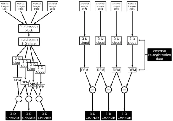
By making the assumption that a sufficient number of keypoints re-main invariant across each time period, our method brings a novelty in the photogrammetric processing of multi-temporal datasets. It con-sisted of processing, at the very first step, all of the images in a single block for the estimation of the interior and exterior orientations. Im-ages of different epochs were then separated and the dense matching steps were performed with images of the same epoch.
In order to test the impact of this method, the other ’classical’ strat-egy was also tested. This stratstrat-egy consists in not using the single block with all images of the different epoch in the the first estimation of in-terior and exin-terior orientations. We hence tested a processing where each epoch was handled separately from the beginning to the end of the SfM-MVS process. The principle of the proposed method as com-pared with the ’classical’ strategy is depicted in Figure2.
2.2.3. Use of additional manually marked points
Different numbers and types of additional - relative to the automatic tie points - manually marked points were used in the different process-ing scenarios, with a minimal set of 9 GCPs to scale and orient the estimated DEMs and DoDs.
The first option, namely, 9 GCPs, corresponded to this minimal set of 9 additional manual GCPs. For the second option, namely, 200
tie points, we added manually marked tie points to reach a total of 200
points. For the third option, namely, 200 GCPs, the ground coordinates of all of the 200 points were also given and used in the SfM workflow. For all of these three options, the manually marked points were added to the set of automatic tie points.
The additional 200 points consisted of carefully chosen permanent ground features, for example road intersections or small rocks, which were manually determined in the images. The corners of buildings or large rocks were avoided to allow the less possible variations of the z coordinate to occur around the chosen points. First, a regular sampling of 200 locations over the whole image block area was de-termined and each of the 200 points was chosen within this regular grid to ensure a homogeneous point density (Figure1). Each of the 9 or 200 points was manually determined in the aerial images of the four epochs. When used as GCP, (x, y, z) ground coordinates were necessary. Considering that our aim was to test methods with limited input, we used existing information and avoided costly and cumber-some field surveys of high-quality reference points. The required co-ordinates were hence collected on the French geographic survey portal on which orthorectified imagery and DEM can be browsed (https: //www.geoportail.gouv.fr/). Empirical observations during the marking of the 200 points in multi-date aerial images resulted in esti-mated accuracy values of 20 m for the ground accuracy and 5 pixels for the image accuracy (Table ??above). The total processing time for determining and assigning the coordinates on 200 locations in 163 images was approximately twenty hours.
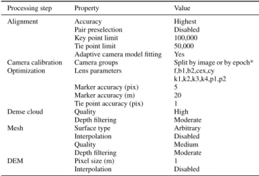
Table 2: Parameters used in PhotoScan Pro c. *Depending on the
autocalibra-tion opautocalibra-tion (see2.2.4).
Processing step Property Value
Alignment Accuracy Highest
Pair preselection Disabled Key point limit 100,000 Tie point limit 50,000 Adaptive camera model fitting Yes
Camera calibration Camera groups Split by image or by epoch* Optimization Lens parameters f,b1,b2,cex,cy
k1,k2,k3,k4,p1,p2 Marker accuracy (pix) 5
Marker accuracy (m) 20 Tie point accuracy (pix) 1
Dense cloud Quality High
Depth filtering Moderate
Mesh Surface type Arbitrary
Interpolation Disabled
Quality Medium
Depth filtering Moderate
DEM Pixel size (m) 1
Interpolation Disabled
2.2.4. Autocalibration
The autocalibration method aims keeping track of whether all im-ages from a single epoch were taken by the same camera or not. The option by epoch consisted of using a single camera model for all of the images from a given epoch whereas the second option, by image, consisted of entering one camera model for each image. This second option aimed at providing a workaround to the interior orientation is-sue when the pre-processing option is not ’ReSampFid’. With a view to make a multi-factorial comparison, the lens distortion estimations were in all cases made with the same parameter set, which was sug-gested by PhotoScan Pro c (Table??).
2.3. DEMs and DoDs computing - fixed parameters
For all processing scenarios tested, DEM computing was performed with AgiSoft Photoscan Pro c 1.2.6 with the same parameters (Table
??). The first step of the AgiSoft Photoscan Pro SfM-MVS workflow is image alignement. As noticed also byCogliati et al.(2017), highest accuracies were necessary for succeeding in this step with archival im-agery. This step uses an automated image feature detection and match-ing which is comparable to SIFT (Semyonov,2011). Based on the automatically matched points between the images, the image interior and relative exterior orientations were computed. Then, an optimisa-tion step in which the autocalibraoptimisa-tion was refined was performed. For the ’by epoch’ autocalibration option (section2.2.4), estimated lens pa-rameters were the same for all the images taken with the same camera and were distinct between the different cameras. For the ’by image’ au-tocalibration option, estimated lens parameters were different for each image. Depending on the different processing options described above in section2.2.3, additional manually marked GCPs and/or tie points could be used in this step. Once the image block geometry was refined, the dense image matching step was done and resulted in the estimation of a dense 3-D point cloud. Finally, DEMs were exported with a 1 m ground sampling distance with disabled interpolation to avoid subse-quent processing artefacts in the DoDs. DoDs were finally computed by subtracting two successive DEMs. No-data values in at least one of the two input DEMs resulted in no-data values in the computed DoD.
Figure 2: Principle of the proposed method. Left : use of a single block which joins multi-epoch images in the first step of the SfM processing. The whole dataset shares the same unique geometry since the beginning of the workflow. Right : processing workflow when not using the proposed method ; each epoch has a different geometry and co-registration relies on external data, either on GCPs during alignment either with co-registration of obtained DEM on external lidar DEMs or vector data.
2.4. Quality assessment 2.4.1. Validation data
Two external DEMs obtained at different epochs and with differ-ent methods were used for quantitative independdiffer-ent validation. Both these validation DEMs - as well as the DEMs we produced - were in Lambert-93, the official French projection (EPSG:2154). A pho-togrammetric survey of the area conducted in 2012 by Topogeodis pro-vided a DEM with a pixel resolution of 5 m (the larger DEM on Figure
1). Its planimetric accuracy is estimated at 50 cm. The altimetric ac-curacy is estimated at 30 cm in urban zones and at 1 m in mountainous and woodland areas. In 2001, a lidar survey was conducted by Geolas Consulting on a subarea of 7 km2(the smaller area bordered by dashed
lines in Figure1). From these data, a DEM with a pixel resolution of 1 m and an estimated altimetric accuracy of 30 cm was derived.
2.4.2. Quantitative indices
The impact of the different processing options on the results was evaluated with four different metrics. The first metric, ’Image block RMSE’, was based on the internal coherence of the image block es-timated geometry. It consisted of calculating the global RMSE of the bundle block adjustment. It was computed for the 144 image blocks. The second metric, ’Coarse DEM error’, was computed using, as a reference, the 2012 photogrammetric DEM, which covers the whole test site (Figure1). The reference DEM and all of the 144 SfM-MVS DEMs were first resampled at 50 m with bilinear interpolation. The ’Coarse DEM error’ was then computed as the mean absolute differ-ence between the simulated and referdiffer-ence DEMs. This metric was chosen to evaluate whether the computed DEMs of each epoch were coherent with the actual topography. This metric was computed at a 50 m resolution considering that potential 3-D change would be negli-gible at this resolution and has hence been computed for each epoch. The third metric, ’Fine DEM error’ was computed with the 2001 lidar
DEM, which covers a smaller part of the test site as shown in Figure
1. It aimed at checking whether the fine scale topography was cor-rectly estimated by the SfM-MVS DEMs. For the ’Coarse DEM error’, the metric was computed as the mean absolute difference between the simulated and reference DEMs. Considering that, at this scale, 3-D change could not be neglected, this metric was evaluated only on the 36 DEMs that were computed with the images of the year 2001. The fourth metric, ’DoD quality’, corresponded to the internal quality of the computed DoDs, which was estimated by the mean absolute value of the DoD. These metrics are summarised in Table3.
For all of these metrics, we examined whether the different process-ing options described in section2.2had a significant impact on the distribution of the metric or not. Due to the strong skew of the metrics distributions, we used the Kruskal-Wallis test to determine the signifi-cance of the observed differences.
2.4.3. Qualitative analyses of the DoDs
We visually examined all 108 DoDs at a coarse scale to explain the quantitative results obtained with the scalar metrics. We also examined the topographic profiles of the different DEMs to better understand the results obtained on the DoDs. These profiles were extracted on the two transects drawn in Figure1. The best DoDs - in the sense of the ’DoD quality’ metric as described above - were obtained with less external information (only 9 GCPs) and were finally visually examined at full resolution. The detected change signals were associated with actual 3-D change that could be confirmed by other evidence, either exter-nal documentation, or image information. Amongst the 3-D change detected, we examined 3-D change that were linked to anthropogenic activity, such as urban growth, or civil engineering around highways, quarries and backfills. These analyses aimed at validating the potential of the proposed method for detecting and characterising 3-D change with frugal ground information.
Table 3: Metrics used for the evaluation of the different processing options.
Name Unit Samples Description
Image block RMSE pixels 144 Image blocks Bundle block adjustment RMSE
Coarse DEM error metres 144 DEMs Coarse resolution mean absolute difference between the resampled SfM-MVS DEMs and reference DEM Fine DEM error metres 36 DEMs Mean absolute difference between the 2001 SfM-MVS DEM and the fine resolution reference lidar DEM DOD quality metres 108 DoDs Mean of the DoD absolute values
3. Results
3.1. Quantitative assessment
The main parameters of the metrics distributions are shown in Table
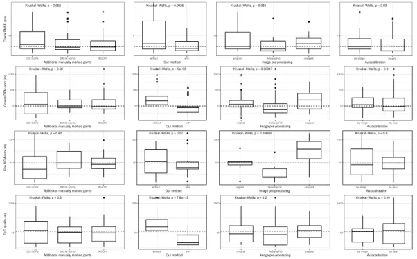
4. For more detail, distribution boxplots are given in Appendix (Figure
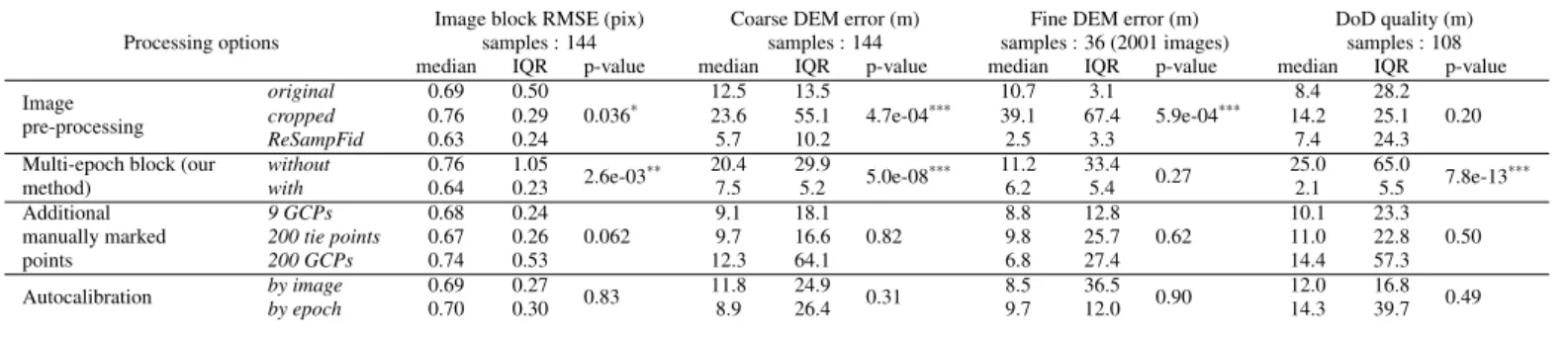
A.9). These results exhibit two groups of processing options that had a significant impact on all of the metrics: the image pre-processing options and the fact of joining multi-epoch images in a single block at first (our proposed method). The most significant result is that with our method, the median DoD quality value lowered to 2.1 m, within an inter-quartile range of 5.5 m, compared to a median DoD qual-ity value of 25.0 m (inter-quartile range of 65.0 m) for all of the 54 DoDs computed without our method. For all of the metrics, using our method allowed us to achieve better quality, and this result was signif-icant for 3 metrics over 4. Second, using the ReSampFid option for image pprocessing also significantly and positively impacted the re-sults by lowering the Coarse DEM error and Fine DEM error to 5.7 m and 2.5 m, respectively. Third, and as testified by the negligible signif-icances for this group of options, adding manually marked points had a negligible impact on the quality of the DEMs and DoDs. Furthermore, the results obtained with these different options were contradictory be-tween metrics. With even worse p-values, autocalibration options also appeared to have had a negligible impact on all of the metrics.
In absolute values, using our proposed method is also the process-ing option that resulted in the best DoD quality, in terms of both the median and inter-quartile range. In addition, the ReSampFid option resulted in the best individual DEMs at both fine and coarse scale. Our experiments hence showed that first the fact of joining multi-epoch im-ages in a single block and then the image pre-processing, had the most significant impacts on the DEMs and DoDs. The ReSampFid option appears to be the most important to obtain the best individual DEMs whereas the best DoDs were obtained by using our method. This find-ing could be because accurate DEMs do not necessarily result in accu-rate DoDs when DEM geometries were not sufficiently coherent.
3.2. Qualitative assessment
Figure3shows the thumbnails of all of the 108 DoDs obtained with the different processing options. First, a few DoDs show spatial pat-terns that are very far from what would be expected. These flawed DoDs, some showing issues with point cloud completeness, corre-spond to situations in which photogrammetric processing converged to an erroneous solution, most likely because of the SfM processing step, but maybe also due to the chosen parametrisation of the dense matching step. For some combinations of processing options, such as using 200 GCPs, not joining multi-epoch images in a single block and performing autocalibration by epoch, almost no solution could be found, regardless of the image pre-processing options.
A strong concave or convex ’doming’ effect (James and Robson,
2014) can be observed for several DoDs that where computed without using our proposed method. These findings give indications about the problems that could have occurred during the SfM processing step, in particular erroneous autocalibration.
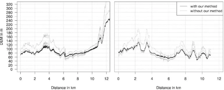
Figure4compares - on two transects - the topographic profiles of
Figure 3: Effect of the different processing options on the DoDs computed (a) with our proposed method and (b) with ’classical’ processing strategies. The figure reads as follows : for example the black-bold framed DoD shows the estimated elevation differences between 1981 and 1990 which was computed by using a single multi-epoch block, using 200 tie points, the cropped pre-processing option and the autocalibration with one lens model by epoch. All of the DoDs are represented with the same colour scale truncated at ±10 m so that extreme values of some DoDs would not hinder the view of smaller dy-namics, 10 meters being the order of magnitude immediately superior to the best DoD quality values (see Table4).
Table 4: Effects of the processing options on the image block quality, DEM quality and DoD quality. For each metric, the total sample number is recalled and the median value, inter-quantile range (IQR) and p-value of the Kruskal-Wallis test for the significance of the differences of the medians is given.
Image block RMSE (pix) Coarse DEM error (m) Fine DEM error (m) DoD quality (m) Processing options samples : 144 samples : 144 samples : 36 (2001 images) samples : 108
median IQR p-value median IQR p-value median IQR p-value median IQR p-value Image
pre-processing
original 0.69 0.50 12.5 13.5 10.7 3.1 8.4 28.2 cropped 0.76 0.29 0.036* 23.6 55.1 4.7e-04*** 39.1 67.4 5.9e-04*** 14.2 25.1 0.20
ReSampFid 0.63 0.24 5.7 10.2 2.5 3.3 7.4 24.3 Multi-epoch block (our
method)
without 0.76 1.05
2.6e-03** 20.4 29.9 5.0e-08*** 11.2 33.4 0.27 25.0 65.0 7.8e-13***
with 0.64 0.23 7.5 5.2 6.2 5.4 2.1 5.5 Additional manually marked points 9 GCPs 0.68 0.24 9.1 18.1 8.8 12.8 10.1 23.3 200 tie points 0.67 0.26 0.062 9.7 16.6 0.82 9.8 25.7 0.62 11.0 22.8 0.50 200 GCPs 0.74 0.53 12.3 64.1 6.8 27.4 14.4 57.3 Autocalibration by image 0.69 0.27 0.83 11.8 24.9 0.31 8.5 36.5 0.90 12.0 16.8 0.49 by epoch 0.70 0.30 8.9 26.4 9.7 12.0 14.3 39.7
the best DEMs computed with and without our method. The DoDs that correspond to these DEMs are marked, respectively, by blue and red rectangles in Figure3. We observed that profiles obtained at different epochs with our method cannot be distinguished between each other on the graph, whereas profiles obtained without our method are clearly distinct. On all profiles, the topographic shapes are locally correctly rendered within all DEMs, but with large and non-stationary biases in the DEMs computed without our method. We also observed that the extent of bias varies along the profile, particularly for the East-West transect where significant biases are recorded in the first 6 km of the profile and beyond 11 km, while biases are significantly reduced between 6 km and 11 km. This spatial pattern may be due to the fact that image orientations may theirselves be estimated with differing bias along the profiles. It would explain that the spatial autocorrelation of the DEMs seem to be of the order of magnitude of the image footprints which is several kilometres.
Finally we selected the best DoDs among those obtained by us-ing our method and the less additional external information. It cor-responded to the association of ReSampFid, 9 GCPs options and auto-calibration by epoch. On these DoDs at full resolution, we sought 3-D change signals and inspected them.
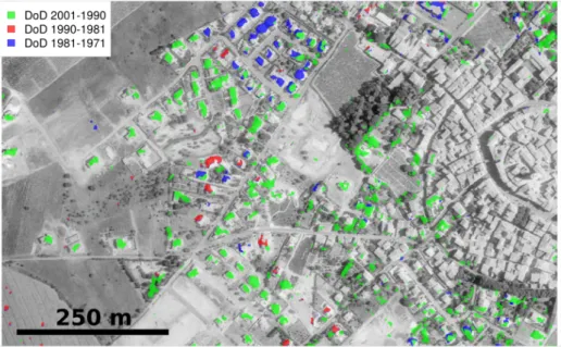
First, we looked for evidences which would demonstrate unambigu-ously that these 3-D changes are not processing artefacts. Figure5
shows excavation (red) and fill (blue) patterns that are clearly super-imposed on the newly constructed highway. This figure demonstrates the capability of detecting 3-D change in DoDs computed with our method and hence with limited external information, considering that we only used 9 GCPs, extracted from already available data. This fig-ure also shows that, even if most of the area contains 3-D difference information, processing may fail. In this zone, difficulty was encoun-tered when addressing low-texture areas, vegetation, some parts of ur-ban areas, and some field plots.
Figure6allows us to detail the potential of these DoDs in terms of the spatial resolution. It shows the DoDs thresholded above 2.5 m and superimposed on the 2001 orthophoto. Rectangular patterns in these thresholded DoDs show strong correlations with the floorspace of the houses that were built within the period. This figure also shows artefacts that could be either small and isolated patches, or thin patterns at the edges of sharp objects.
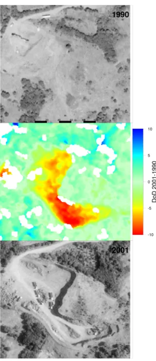
Figures 7and 8allows us to detail the potential of the obtained DoDs in terms of the volume quantification. These figures represent, respectively, the ground excavating and the filling of a limited area. These two types of 3-D change could not be detected from orthophotos alone, in terms of volume quantification and even for the delineation of the impacted zone. This aspect is especially depicted in Figure8, where changes in the texture have a larger extent than changes in the surface height.
4. Discussion
The objective of this work was to evaluate the potential of a new method - which relies on the use of a single multi-epoch image block in the first steps of SfM processing - to compute informative DEMs of difference with limited photogrammetric expertise and almost exclusively image information.
After a thorough exploration of different processing strategies, we showed that the use of our method allowed for computing DoDs in which actual 3-D change could be detected and quantified. Moreover, the proposed method played the most significant role to ensure the computation of high-quality DoDs. To the best of our knowledge, au-tomated computation of multi-temporal feature points for DoD esti-mation by feeding SIFT-like algorithms with multi-temporal datasets has not yet been assessed.Hapke(2005),Korpela(2006) andDewitte et al.(2008) already used multi-temporal tie points for this purpose but these points were manually marked. Fox and Cziferszky(2008) computed tie points between images from different epochs and even thought about a method similar to the one proposed in this paper in what they called a simultaneous ’grand adjustment’. However, even if these authors appreciated this possible method as elegant, they re-jected this option to keep the quality of the reference block geometry and to avoid difficult posterior error checks. Thus, even if temporal SIFT methods are common in computer vision for the processing of videos, to the best of our knowledge only two authors have proposed studies with experiments that showed some similarity to our method. In a study that aims at characterising the yearly evolution of the snow-line,Vargo et al.(2017) used SfM photogrammetry to process a multi-temporal dataset of aerial imagery with at least one image per year from 1981 to 2017. Because for some years, only one image was available, they have had to put images from different epochs in the same block. Nevertheless, they also have had to mask snow and ice out of all images in such a way that the algorithm could estimate the orientations of these isolated images. Chanut et al.(2017) also suc-cessfully used a SfM algorithm to compute tie points between images from different epochs in a study that aimed at quantifying 3-D move-ments on a landslide. Multi-temporal tie points were used to initialise a dense correlation step. Mass movements were finally quantified from the results of the dense correlation.
The second most important finding is that pre-processing of scanned analogue imagery also plays a prime role in the next processing steps of SfM-MVS. This finding is consistent with the existing literature that addressed the use of archival aerial imagery with SfM algorithms.
Salach(2017) developed a specific software to resample scanned ana-logue photographs relative to information given by fiducial marks. These authors tested different processing strategies: with or with-out pre-processing, and with different GCP numbers and
configura-Figure 4: Profile comparison between the best DEMs computed respectively with (in black) and without (in grey) our proposed method. Each line corresponds to a different epoch. Left, the East-West transect ; right, the North-South transect (see transects on Figure1).
Figure 5: 3-D change associated with highway construction. The 1990-1981 DoD is superimposed on the 1990 orthophoto. Colourless areas correspond to areas where no value was computed in the DoD. The DoD was estimated with our proposed method, using 9 GCPs, autocalibration with a unique camera model by epoch and the ReSampFid pre-processing.
tions. They reported that initial estimates of image orientations with this processing were better than those obtained without this pre-processing. More, the results with pre-processing and a minimal GCP set were similar to the results without pre-processing but with a com-plete set of GCPs. The latter result is hence corroborated by the results of our study. Gonc¸alves(2016) used a manual affine transformation that was computed on the position of the fiducial marks to register the scanned analogue images with one another. This step allowed the use of archival aerial imagery in SfM workflow for automated mosaicking and DEM production. The RMSE of the obtained DEM, of 4.7 m, is of the same order of magnitude than the DEM errors estimated in our study.Cogliati et al.(2017) also used SfM software to compute DEMs and DoDs from historical aerial imagery and transformed scanned im-ages so that fiducial marks would be positioned in the corner of the resampled images, which hence shared the same geometry. After an additional step of co-registration on an external high-scale vector map, they computed DoDs and compared their results with Lidar data. On stable zones, they obtained mean DoD values ranging from -9.88m to +18.17m. Nocerino et al.(2012) also exploited the fiducial marks to establish an image reference coordinate system at the geometrical cen-tre of the fiducial marks. The RMSE estimated on the z coordinates of the check points ranged from 7 m to 10 m. Our results hence compare favourably with these estimated decametric accuracies.
The third finding can be seen as being more unexpected : our experi-ments showed that the use of a relatively high number of added manual GCPs and/or tie points appears to play a negligible role on the image blocks, DEMs, and DoDs quality. This finding appears to be in contra-diction to the results of previous studies based on the thorough use of GCPs to compute DoDs from archival aerial imagery. Indeed,Hapke
(2005);Zanutta et al.(2006);Dewitte et al.(2008);Fox and Czifer-szky(2008);Micheletti et al.(2015);Papworth et al.(2016);Mertes et al.(2017) successfully used GCPs of different sources to ensure a geometrical consistency between DEMs before subtracting them from each other. This apparent contradiction can be explained by the fact that these studies used a method that significantly differs from ours. In contrast to these studies, we performed fully automatic photogrammet-ric processing, from image block orientation to DEM extraction and DoD computing. With the aim of being able to apply our method to
Figure 6: Superimposition of thresholded DoDs (values greater than 2.5 m) onto the 2001 orthophoto (gray levels). The DoDs were estimated with our proposed method, using 9 GCPs, autocalibration with a unique camera model by epoch and the ReSampFid pre-processing.
large image data sets, we did not performed any manually checking of the results at any intermediary steps. As a consequence, we eventually missed gross GCP errors, such as the errors mentioned, for example, by Verhoeven and Vermeulen(2016), who iteratively eliminated the GCPs that caused largest errors. In our case, this uncontrolled use of additional manually marked points resulted in flawed DoDs for some of the processing option combinations. According toCogliati et al.
(2017), these issues may also come from the parameter choices. These authors indeed reported that completeness of the final point cloud may be jeopardized when using too high ’Quality’ parameters in the dense matching step - even if the alignment was computed with the ’Highest’ accuracy parameter as also recommended by these authors. The syn-thesis of our results and the results in the literature is that both cum-bersome manual marking in all images and a time-consuming man-ual check of image orientation results are required to enable manman-ually marked GCPs to improve the photogrammetric processing.
In our opinion, the fact that our method allows for a correct compu-tation of the DoDs has at least two explanations. The first explanation is linked to the use of the tie points that were computed between im-ages of different epochs. Image block geometries of different epochs are hence coherent by construction and consequently, the DEM spatial references are consistent and allow for a proper estimation of their dif-ferences. The second explanation is linked with autocalibration. We postulate that our method also has benefits for the SfM autocalibration step. Autocalibration of archival aerial imagery can indeed be sen-sitive, as noted, for example, byAguilar et al.(2013), and it can be even more difficult with SfM algorithms. This finding is due to the geometry of the archival image acquisitions and its inadequacy with respect to the requirements of the SfM algorithms. First, overlaps in archival aerial imagery are small (60%) compared to the overlaps re-quired for the SfM algorithms (80%, or even 90%). Second, in our study, with altitudes higher than 2700 metres and height differences on the ground of less than 400 m, the ground is mostly flat relative to the flying height. As a consequence, acquisition geometry of archival aerial imagery constitutes a non-ideal case for autocalibration, with strong possible correlations between estimated interior and exterior orientations, in particular the flying height and focal length. This
cor-relation could result in the doming effect observed byJames and Rob-son(2014) on UAV images, which we also observed in some of the processing scenarios. One explanation may be that autocalibration in a same image block of the four cameras used at four different epochs would in most cases allow for a lesser correlation of interior and ex-terior orientation. This may however not be the case if some epochs, for instance with lesser quality images or particularly ill-conditioned image canvas, would bring and propagate bias or noise to the whole multi-temporal block through the bundle adjustment. Further develop-ment on the method may be needed to improve its robustness to such cases.
This said, qualitative analyses of the DoDs obtained with our proposed method also demonstrated its potential. DoDs obtained using a limited number of GCPs indeed unambiguously detected and quantified past 3-D change. As orthophotos greatly changed in texture and grey levels from year to year due to the significant evolution of land management and land cover on the area (Vinatier and Arnaiz,
2018), the use of DoDs allowed us to detect 3-D change that would most likely be missed by orthophoto analysis. It is also worthwhile to note that the magnitudes of the changes mapped by our method are small relative to the changes observed with DoDs on volcanoes (e.g.
Gomez, 2014) and on glaciers (e.g.Mertes et al., 2017;M¨olg and Bolch,2017). To the best of our knowledge, onlyBakker and Lane
(2017) presented results with 3-D change that was smaller than ±3 metres. To achieve this precision, they used an external lidar dataset and the a priori knowledge of stable areas for the fine co-registration of multi-temporal DEMs. Furthermore, the study of anthropogenic changes from DoDs rather than orthophotos is rarely encountered in the literature, except inCogliati et al.(2017) andSevara et al.(2017). The latter succeeded in mapping 3-D change related to quarries thanks to a fine co-registration of each DEM with an external lidar DEM prior to photogrammetric DEMs differencing, though.
With extensive testing of different processing scenarios, we showed that our proposed method can be advantageous for a first blind ex-ploration of archival aerial imagery for the detection of 3-D change. Even though our studies already cover a time span of three decades
Figure 7: 3-D change associated with excavation activities in a quarry. Top: the 1990 orthophoto. Middle, the 2001-1990 DoD. Colourless areas correspond to areas where no value was computed in the DoD. The DoD was estimated with our proposed method, using 9 GCPs, autocalibration with a single camera by epochand the ReSampFid pre-processing. Bottom: the 2001 orthophoto.
Figure 8: 3-D change associated with ground filling. Top: the 1971 orthophoto. Middle, the cumulated 2001-1971 DoD. Colourless areas correspond to areas where no value was computed in the DoD. The DoD was estimated with our proposed method, using 9 GCPs, autocalibration with a unique camera model by epochand the ReSampFid pre-processing. Bottom: the 2001 orthophoto.
and an area of 170 km2, the results can be different in the case of
other time spans and/or on other sites, in particular, on sites that would exhibit even larger changes than ours. Nevertheless, our method can conveniently and inexpensively be used first, with no other informa-tion other than image informainforma-tion, to detect zones with 3-D change. This approach - using a first single block with multi-epoch images and no GCP - was already successfully tested (Feurer et al.,2017). It can favourably be used with datasets of thousands of images. Users inter-ested in a more detailed and accurate description of 3-D change can then use additional information and/or a dedicated workflow focused on the zones in which 3-D change would have been detected with our method and no GCP at all. However, our method may also result in the computation of a significant number of ’unstable’ multi-temporal tie points, for example in the case of a large translation landslide. In the corresponding zone, camera positions and then 3-D information would then be incorrectly estimated, which may in turn be a clue for detecting large mass movements. Indeed, the success of our proposed method relies on the fact that stable multi-temporal tie points are pre-dominant in the image space. As stated above, this criteria may not be verified in landscapes where change is large relatively to the spatio-temporal scale of the available imagery.
Other future work should hence test the robustness of the proposed method on larger time spans and different landscape types. Some im-provement can also be done on the interior orientation step. First, the method may advantageously be tested with images for which the de-tection of fiducial marks available in AgiSoft Photoscan Pro csince the
1.4.3 version would succeed - i.e., with images newer than the eight-ies. Second, when taking into account the information given by fiducial marks (the ReSampFid option in our case), a simpler lens model -or even no c-orrection of the lens dist-ortion - may favourably be tested in the case of high-quality metric cameras. Third, a better model of the camera inner orientation may be estimated by using more fidu-cial marks than the 4 marks of the corners. Fourth, there is still a need to find methods that would allow for the use of archival aerial imagery scanned with desktop scanners instead of a photogrammetric scanner. This approach would necessitate the use of more informa-tion from the scanned analogue image borders for example, in order to determine a model of the scanner deformation. Finally, the proposed method may also be successful on other multi-temporal datasets than archival aerial imagery. The principle of using a single image block with multi-epochs images can indeed be exploited with virtually any multitemporal dataset and would be worth tested on any of these cases.
5. Conclusions
In this paper, we proposed and tested a new method which allows for the detection of 3-D change from archival aerial imagery with most exclusively image information. We showed that this method al-lowed for the computing of informative DEMs of differences, in which 3-D change could be detected and characterised. Because it can be applied automatically and does not require either photogrammetric ex-pertise or additional data, this new method can pave the way to a more extensive use of the worldwide aerial imagery archive. This method hence constitutes an additional tool in geosciences for the detection of past 3-D change. This work sets the stage of two types of new studies. First this method should be tested in different contexts and with other image datasets including any digital multi-temporal imagery to deter-mine its robustness. Second, the worldwide archival aerial imagery can be explored with the proposed method in such a way that past 3-D change can be discovered or characterised.
The base hypothesis of our work was to lessen as much as possible the use of external data and to make available to a broader audience the multi-temporal 3-D information of archival aerial imagery. Our
work hence focused on easily available and/or inexpensive data and methods. This approach indeed meets a prime criteria in such a way that it can further be applied on larger datasets within as many different contexts as possible and by the most extensive community.
Acknowledgements
This research was supported by the French National Research Agency (ANR) through the ALMIRA project (ANR-12-TMED-0003) and was done in the frame of the Tunisian-French joint international laboratory NAILA (http://www.lmi-naila.com/). The authors thank the IGN for having made freely available the archival aerial imagery, Nico-las Devaux for helpful discussions on the processing and warmfully express their gratitude to the two anonymous reviewers for their help on the manuscript, especially for the acute and insightful remarks on photogrammetric processing.
References
D. C. Cowley, B. B. Stichelbaut, Historic Aerial Photographic Archives for Eu-ropean Archaeology, EuEu-ropean Journal of Archaeology 15 (2) (2012) 217– 236, ISSN 1461-9571,doi:10.1179/1461957112Y.0000000010.
G. Verhoeven, Taking computer vision aloft–archaeological three-dimensional reconstructions from aerial photographs with photoscan, Archaeological prospection 18 (1) (2011) 67–73.
C. Sevara, Top Secret Topographies: Recovering Two and Three-Dimensional Archaeological Information from Historic Reconnaissance Datasets Us-ing Image-Based ModellUs-ing Techniques, International Journal of Heritage in the Digital Era 2 (3) (2013) 395–418, ISSN 2047-4970, doi:10.1260/
2047-4970.2.3.395.
G. Verhoeven, F. Vermeulen, Engaging with the Canopy¢Multi-Dimensional Vegetation Mark Visualisation Using Archived Aerial Images, Remote Sens-ing 8 (9) (2016) 752,doi:10.3390/rs8090752.
A. Salach, SAPC - Application for adapting scanned analogue photographs to use them in structure from motion technology, International Archives of the Photogrammetry, Remote Sensing & Spatial Information Sciences 42. C. Sevara, G. Verhoeven, M. Doneus, E. Draganits, Surfaces from the
Vi-sual Past: Recovering High-Resolution Terrain Data from Historic Aerial Imagery for Multitemporal Landscape Analysis, Journal of Archaeological Method and Theory ISSN 1573-7764,doi:10.1007/s10816-017-9348-9. C. Gomez, Y. Hayakawa, H. Obanawa, A study of Japanese landscapes using
structure from motion derived DSMs and DEMs based on historical aerial photographs: New opportunities for vegetation monitoring and diachronic geomorphology, Geomorphology 242 (Supplement C) (2015) 11 – 20, ISSN 0169-555X,doi:https://doi.org/10.1016/j.geomorph.2015.02.021. J. A. Gonc¸alves, Automatic orientation and mosaicking of archived aerial
pho-tography using structure from motion, ISPRS - International Archives of the Photogrammetry, Remote Sensing and Spatial Information Sciences XL-3/W4 (2016) 123–126,doi:10.5194/isprs-archives-XL-3-W4-123-2016. S. Ishiguro, H. Yamano, H. Oguma, Evaluation of DSMs generated from
multi-temporal aerial photographs using emerging structure from motion¢multi-view stereo technology, Geomorphology 268 (2016) 64–71.
M. Bakker, S. N. Lane, Archival photogrammetric analysis of river-floodplain systems using Structure from Motion (SfM) methods, Earth Surface Pro-cesses and Landforms 42 (8) (2017) 1274–1286, ISSN 1096-9837, doi:
10.1002/esp.4085.
J. R. Mertes, J. D. Gulley, D. I. Benn, S. S. Thompson, L. I. Nicholson, Using structure-from-motion to create glacier DEMs and orthoimagery from historical terrestrial and oblique aerial imagery, Earth Surface Pro-cesses and Landforms 42 (14) (2017) 2350–2364, ISSN 1096-9837,doi:
10.1002/esp.4188.
N. M¨olg, T. Bolch, Structure-from-Motion Using Historical Aerial Images to Analyse Changes in Glacier Surface Elevation, Remote Sensing 9 (10), ISSN 2072-4292,doi:10.3390/rs9101021.
L. J. Vargo, B. M. Anderson, H. J. Horgan, A. N. Mackintosh, A. M. Lor-rey, M. Thornton, Using structure from motion photogrammetry to measure past glacier changes from historic aerial photographs, Journal of Glaciology 63 (242) (2017) 1105–1118, ISSN 0022-1430, 1727-5652,doi:10.1017/jog.
2017.79.
C. Gomez, Digital photogrammetry and GIS-based analysis of the bio-geomorphological evolution of Sakurajima Volcano, diachronic
analy-sis from 1947 to 2006, Journal of Volcanology and Geothermal Re-search 280 (Supplement C) (2014) 1–13, ISSN 0377-0273,doi:10.1016/j.
jvolgeores.2014.04.015.
S. N. Lane, R. M. Westaway, D. M. Hicks, Estimation of erosion and depo-sition volumes in a large, gravelbed, braided river using synoptic remote sensing, Earth Surface Processes and Landforms 28 (3) (2003) 249–271,
doi:10.1002/esp.483.
J. M. Wheaton, J. Brasington, S. E. Darby, D. A. Sear, Accounting for uncer-tainty in DEMs from repeat topographic surveys: improved sediment bud-gets, Earth Surface Processes and Landforms 35 (2) (2010) 136–156. R. Williams, DEMs of difference, Geomorphological Techniques 2 (3.2). K. Kraus, P. Waldh¨ausl, Manuel de photogramm´etrie: principes et proc´ed´es
fondamentaux, Herm`es, 1998.
M. Fabris, A. Pesci, Automated DEM extraction in digital aerial photogram-metry: precisions and validation for mass movement monitoring, Annals of Geophysics 48 (6).
L. Fischer, H. Eisenbeiss, A. K¨a¨ab, C. Huggel, W. Haeberli, Monitoring topo-graphic changes in a periglacial high-mountain face using high-resolution DTMs, Monte Rosa East Face, Italian Alps, Permafrost and Periglacial Pro-cesses 22 (2) (2011) 140–152.
N. Micheletti, S. N. Lane, J. H. Chandler, Application of archival aerial pho-togrammetry to quantify climate forcing of alpine landscapes, The Pho-togrammetric Record 30 (150) (2015) 143–165, ISSN 1477-9730, doi:
10.1111/phor.12099.
P. P. C. Aucelli, M. Conforti, M. Della Seta, M. Del Monte, L. D’uva, C. M. Rosskopf, F. Vergari, Multi-temporal Digital Photogrammetric Analysis for Quantitative Assessment of Soil Erosion Rates in the Landola Catchment of the Upper Orcia Valley (Tuscany, Italy), Land Degradation & Development 27 (4) (2016) 1075–1092, ISSN 1099-145X,doi:10.1002/ldr.2324. K. D. Fieber, J. P. Mills, P. E. Miller, L. Clarke, L. Ireland, A. J. Fox,
Rig-orous 3D change determination in Antarctic Peninsula glaciers from stereo WorldView-2 and archival aerial imagery, Remote Sensing of Environment 205 (2018) 18–31.
J. H. Chandler, M. A. R. Cooper, The extraction of positional data from historical photographs and their application to geomorphology, The Pho-togrammetric Record 13 (73) (1989) 69–78,doi:10.1111/j.1477-9730.1989.
tb00647.x.
J. Walstra, N. Dixon, J. Chandler, Historical aerial photographs for landslide assessment: two case histories, Quarterly Journal of Engineering Geology and Hydrogeology 40 (4) (2007) 315–332, ISSN 1470-9236,doi:10.1144/
1470-9236/07-011.
P. Redweik, V. Garz´on, T. s. Pereira, Recovery of stereo aerial coverage from 1934 and 1938 into the digital era, The Photogrammetric Record 31 (153) (2016) 9–28.
C. Sevara, Capturing the Past for the Future: an Evaluation of the Effect of Geometric Scan Deformities on the Performance of Aerial Archival Media in Image-based Modelling Environments, Archaeological Prospection 23 (4) (2016) 325–334, ISSN 1099-0763,doi:10.1002/arp.1539.
M. A. Aguilar, F. J. Aguilar, I. Fernndez, J. P. Mills, Accuracy Assessment of Commercial SelfCalibrating Bundle Adjustment Routines Applied to Archival Aerial Photography, The Photogrammetric Record 28 (141) (2013) 96–114,doi:10.1111/j.1477-9730.2012.00704.x.
T. D. James, T. Murray, N. E. Barrand, S. L. Barr, Extracting photogram-metric ground control from lidar DEMs for change detection, The Pho-togrammetric Record 21 (116) (2006) 312–328, ISSN 1477-9730, doi:
10.1111/j.1477-9730.2006.00397.x.
C. J. Hapke, Estimation of regional material yield from coastal landslides based on historical digital terrain modelling, Earth Surface Processes and Land-forms 30 (6) (2005) 679–697,doi:10.1002/esp.1168.
O. Dewitte, J.-C. Jasselette, Y. Cornet, M. Van Den Eeckhaut, A. Col-lignon, J. Poesen, A. Demoulin, Tracking landslide displacements by multi-temporal DTMs: a combined aerial stereophotogrammetric and LIDAR ap-proach in western Belgium, Engineering Geology 99 (1-2) (2008) 11–22. A. Zanutta, P. Baldi, G. Bitelli, M. Cardinali, others, Qualitative and
quan-titative photogrammetric techniques for multi-temporal landslide analysis, Annals of Geophysics 49 (4-5).
A. J. Fox, A. Cziferszky, Unlocking the time capsule of historic aerial photogra-phy to measure changes in antarctic peninsula glaciers, The Photogrammet-ric Record 23 (121) (2008) 51–68,doi:10.1111/j.1477-9730.2008.00463.x. S. Nagarajan, T. Schenk, Feature-based registration of historical aerial
im-ages by Area Minimization, ISPRS Journal of Photogrammetry and
Re-mote Sensing 116 (Supplement C) (2016) 15 – 23, ISSN 0924-2716,doi:
https://doi.org/10.1016/j.isprsjprs.2016.02.012.
S. Giordano, A. Le Bris, C. Mallet, Toward automatic georeferencing of archival aerial photogrammetric surveys, ISPRS Annals of Photogramme-try, Remote Sensing and Spatial Information Sciences IV-2 (2018) 105–112,
doi:10.5194/isprs-annals-IV-2-105-2018.
M. Westoby, J. Brasington, N. Glasser, M. Hambrey, J. Reynolds, ’Structure-from-Motion’photogrammetry: A low-cost, effective tool for geoscience ap-plications, Geomorphology 179 (2012) 300–314.
M. A. Fonstad, J. T. Dietrich, B. C. Courville, J. L. Jensen, P. E. Carbonneau, Topographic structure from motion: a new development in photogrammetric measurement, Earth Surface Processes and Landforms 38 (4) (2013) 421– 430, ISSN 1096-9837,doi:10.1002/esp.3366.
D. G. Lowe, Distinctive image features from scale-invariant keypoints, Interna-tional journal of computer vision 60 (2) (2004) 91–110.
A. Eltner, A. Kaiser, C. Castillo, G. Rock, F. Neugirg, A. Abelln, Image-based surface reconstruction in geomorphometry - merits, limits and devel-opments, Earth Surface Dynamics 4 (2) (2016) 359–389, ISSN 2196-6311,
doi:https://doi.org/10.5194/esurf-4-359-2016.
M. Smith, J. Carrivick, D. Quincey, Structure from motion photogrammetry in physical geography, Progress in Physical Geography 40 (2) (2016) 247–275, ISSN 0309-1333,doi:10.1177/0309133315615805.
A. R. Mosbrucker, J. J. Major, K. R. Spicer, J. Pitlick, Camera system consider-ations for geomorphic applicconsider-ations of SfM photogrammetry, Earth Surface Processes and Landforms 42 (6) (2017) 969–986, ISSN 0197-9337,doi:
10.1002/esp.4066, wOS:000400646100010.
M. Cogliati, E. Tonelli, D. Battaglia, M. Scaioni, Extraction of Dems and Orthoimages from Archive Aerial Imagery to Support Project Planning in Civil Engineering, ISPRS Annals of Photogrammetry, Remote Sensing and Spatial Information Sciences IV-5/W1 (2017) 9–16, doi:10.5194/isprs-annals-IV-5-W1-9-2017, URL https: //www.isprs-ann-photogramm-remote-sens-spatial-inf-sci.
net/IV-5-W1/9/2017/.
M. James, S. Robson, S. d’Oleire Oltmanns, U. Niethammer, Optimising {UAV} topographic surveys processed with structure-from-motion: Ground con-trol quality, quantity and bundle adjustment, Geomorphology 280 (2017) 51 – 66, ISSN 0169-555X,doi:http://dx.doi.org/10.1016/j.geomorph.2016.
11.021.
M.-A. Chanut, J. Kasperski, L. Dubois, S. Dauphin, J.-P. Duranthon, Quantifi-cation des dplacements 3D par la mthode PLaS - appliQuantifi-cation au glissement du Chambon (Isre), Revue Franaise de Gotechnique (150) (2017) 4, ISSN 0181-0529, 2493-8653,doi:10.1051/geotech/2017009.
F. Vinatier, A. G. Arnaiz, Using resolution multitemporal imagery to high-light severe land management changes in Mediterranean vineyards, Applied Geography 90 (2018) 115–122, ISSN 0143-6228, doi:10.1016/j.apgeog.
2017.12.003.
D. Feurer, S. Massuel, M. A. El Maaoui, M. R. Boussema, Which 3D changes can be seen with SfM processing of historical aerial imagery?, in: Colloque SFPT Photogrammtrie et tldtection : vers la convergence?, SFPT, 2017. E. Rupnik, M. Daakir, M. Pierrot Deseilligny, MicMac – a free, open-source
so-lution for photogrammetry, Open Geospatial Data, Software and Standards 2 (1) (2017) 14, ISSN 2363-7501,doi:10.1186/s40965-017-0027-2.
D. Semyonov, Algorithms used in PhotoScan [Msg 2],
http://www.agisoft.ru/forum/index.php?topic=89.0, Retrieved June 14, 2018, 2011.
M. R. James, S. Robson, Mitigating systematic error in topographic models de-rived from UAV and ground-based image networks, Earth Surface Processes and Landforms 39 (10) (2014) 1413–1420.
I. Korpela, Geometrically accurate time series of archived aerial images and airborne lidar data in a forest environment, Silva Fennica 40 (1) (2006) 109. E. Nocerino, F. Menna, F. Remondino, C. I. Wg, Multi-temporal analysis of
landscapes and urban areas, 2012.
H. Papworth, A. Ford, K. Welham, D. Thackray, Assessing 3D metric data of digital surface models for extracting archaeological data from archive stereo-aerial photographs, Journal of Archaeological Science 72 (2016) 85–104.
● ● ● ● ● ● Kruskal−Wallis, p = 0.062 1
Chunk RMSE (pix)
Kruskal−Wallis, p = 0.0026 1 without with Our method ● ● ● Kruskal−Wallis, p = 0.036 1
original ReSampFid cropped
Image pre-processing ● ● ● ● ● Kruskal−Wallis, p = 0.83 1 by image by year Autocalibration ● ● Kruskal−Wallis, p = 0.82 10 100 1000 Coar se DEM er ror (m ) ● ● ● ● ● ● ● ● ● ● ● ● ● ● ● ● ● Kruskal−Wallis, p = 5e−08 10 100 1000 without with Our method ● ● ● ● ● ● ● ● Kruskal−Wallis, p = 0.00047 10 100 1000
original ReSampFid cropped
Image pre-processing ● ● Kruskal−Wallis, p = 0.31 10 100 1000 by image by year Autocalibration ● Kruskal−Wallis, p = 0.62 10 100 Fine DE M err or (m ) ● ● ● ● Kruskal−Wallis, p = 0.27 10 100 without with Our method ● ● ● Kruskal−Wallis, p = 0.00059 10 100
original ReSampFid cropped
Image pre-processing Kruskal−Wallis, p = 0.9 10 100 by image by year Autocalibration ● Kruskal−Wallis, p = 0.5 10 1000 DoD q uality (m ) ● Kruskal−Wallis, p = 7.8e−13 10 1000 without with Our method ● Kruskal−Wallis, p = 0.2 10 1000
original ReSampFid cropped
Image pre-processing Kruskal−Wallis, p = 0.49 10 1000 by image by year Autocalibration 200 GCPs 200 tie points 9 GCPs
Additional manually marked points
200 GCPs 200 tie points 9 GCPs
Additional manually marked points
200 GCPs 200 tie points 9 GCPs
Additional manually marked points
200 GCPs 200 tie points 9 GCPs
Additional manually marked points
Figure A.9: Boxplots of (a) alignment quality, (b,c) the difference between computed and reference DEM, respectively the coarse globale and fine local lidar DEM and (d) DoD quality. P-values issued from Kruskal-Wallis tests comparing each modality side-by-side are given.