HAL Id: hal-01344013
https://hal.archives-ouvertes.fr/hal-01344013
Submitted on 15 May 2021
HAL is a multi-disciplinary open access
archive for the deposit and dissemination of
sci-entific research documents, whether they are
pub-lished or not. The documents may come from
teaching and research institutions in France or
abroad, or from public or private research centers.
L’archive ouverte pluridisciplinaire HAL, est
destinée au dépôt et à la diffusion de documents
scientifiques de niveau recherche, publiés ou non,
émanant des établissements d’enseignement et de
recherche français ou étrangers, des laboratoires
publics ou privés.
Insights from a 3-D temperature sensors mooring on
stratified ocean turbulence
Hans van Haren, Andrea A. Cimatoribus, Frédéric Cyr, Louis Gostiaux
To cite this version:
Hans van Haren, Andrea A. Cimatoribus, Frédéric Cyr, Louis Gostiaux. Insights from a 3-D
tem-perature sensors mooring on stratified ocean turbulence. Geophysical Research Letters, American
Geophysical Union, 2016, 43 (9), pp.4483 - 4489. �10.1002/2016GL068032�. �hal-01344013�
Insights from a 3-D temperature sensors mooring
on strati
fied ocean turbulence
Hans van Haren1, Andrea A. Cimatoribus1, Frédéric Cyr1,2, and Louis Gostiaux3
1
NIOZ Royal Netherlands Institute for Sea Research and Utrecht University, Den Burg, Netherlands,2Now at Institut Méditerranéen d’Océanologie (MIO), Marseille CEDEX 9, France,3Laboratoire de Mécanique des Fluides et d’Acoustique, UMR CNRS 5509, École Centrale de Lyon, Université de Lyon, Écully CEDEX 9, France
Abstract
A unique small-scale 3-D mooring array has been designed consisting offive parallel lines, 100 m long and 4 m apart, and holding up to 550 high-resolution temperature sensors. It is built for quantitative studies on the evolution of stratified turbulence by internal wave breaking in geophysical flows at scales which go beyond that of a laboratory. Here we present measurements from above a steep slope of Mount Josephine, NE Atlantic where internal wave breaking occurs regularly. Vertical and horizontal coherence spectra show an aspect ratio of 0.25–0.5 near the buoyancy frequency, evidencing anisotropy. At higher frequencies, the transition to isotropy (aspect ratio of 1) is found within the inertial subrange. Above the continuous turbulence spectrum in this subrange, isolated peaks are visible that locally increase the spectral width, in contrast with open ocean spectra. Their energy levels are found to be proportional to the tidal energy level.1. Introduction
In the stratified ocean, internal waves and turbulent mixing are three-dimensional “3-D” physical processes that are enhanced above sloping topography [Thorpe, 1987]. Knowledge about turbulent mixing properties is important for the (re)distribution of energy, suspended matter, and nutrients, which are indispensable for life. According to near-bottom ocean observations, more than 50% of the turbulent mixing in terms of energy dissipation rate and eddy diffusivity can occur in less than 5% of a dominant wave cycle during the arrival of an upslope propagating and highly nonlinear turbulent bore [van Haren and Gostiaux, 2012]. Such a bore generates a trail of short internal waves close to the local, thin-layer buoyancy frequency. According to numerical and laboratory modeling [e.g., Aghsaee et al., 2010], the bore front may be 2-D in appearance as an interfacial wave or at least have different scales in cross-slope and along-slope dimensions. The same scale difference occurs in turbulence when it is hampered in the vertical by the stable density stratification. Thus far, this has been mainly established for low Reynolds numberflows [Gargett, 1988]. In higher Reynolds number flows, especially those associated with internal wave breaking, turbulent overturn development from the largest to the smallest, dissipative scales is expected to be an essentially 3-D process (similar scales in all three Cartesian coordinates). This raises questions about traditional in situ observations of internal wave turbulence that have so far been made using 1-D moored instrumented lines equipped with high-resolution temperature sensors. In the past, few experiments have been set up in the ocean with two or more instrumented mooring lines at hor-izontal distances of less than 10 km, roughly resolving the correlation length scale of the relevant internal waves. Exceptions were the formidable one-time pyramid experiment of the Internal Wave EXperiment (IWEX) in the open West Atlantic Ocean resolving scales of 6 m [Briscoe, 1975], and, at considerably larger scales O(1–10 km), the deep-sea conventional mooring experiment above the Madeira Basin abyssal plain in the East Atlantic [Saunders, 1983].
The IWEX experiment showed high correlation in the internal wave band between neighboring sensors, but even at the 6 m horizontal scale, a drop in coherence was observed near the local buoyancy frequency of the small-scale internal waves. This drop was not attributed to instrumental deficiency but to nonlinear wave effects [Briscoe, 1975]. A set of 2 Hz sampled acoustic Doppler current profiler (ADCP) observations from half-way up the continental slope in the Bay of Biscay confirmed these decorrelation scales for highly nonlinear turbulent bores that dominate internal wave breaking above sloping topography [van Haren, 2007]. A recent three moorings free-fall dropping experiment done by our team in 2000 m water depth failed in its aim of forming a triangle with horizontal sides of 75 m. The lines were rather at horizontal distances of 200, 180, and 20 m, with an estimated error of 20 m in location determination. The observations proved that
PUBLICATIONS
Geophysical Research Letters
RESEARCH LETTER
10.1002/2016GL068032
Key Points:
• Successful deployment of 3-D temperature sensors mooring in the deep ocean
• Demonstrating the transition from anisotropic to isotropic turbulence and showing coherent portions in the inertial subrange
• Facilitating a better understanding of internal wave breaking and turbulence development which is not easily achievable in the laboratory
Correspondence to:
H. van Haren, hans.van.haren@nioz.nl
Citation:
van Haren, H., A. A. Cimatoribus, F. Cyr, and L. Gostiaux (2016), Insights from a 3-D temperature sensors mooring on stratified ocean turbulence, Geophys. Res. Lett., 43, 4483–4489, doi:10.1002/ 2016GL068032.
Received 29 JAN 2016 Accepted 8 APR 2016
Accepted article online 11 APR 2016 Published online 14 MAY 2016
©2016. American Geophysical Union. All Rights Reserved.
turbulent bore motions certainly decorrelate at the 200 m scale and in the smaller details also at 20 m (unpublished results). This experiment led to the construction of a single multiple-line 3-D mooring array of temperature sensors resolving 1 m vertical and 4 m horizontal scales. After several years of development, trials, and modifications, these innovative measurements are presented here focusing on statistics of the internal wave turbulence band.
2. Technical Details
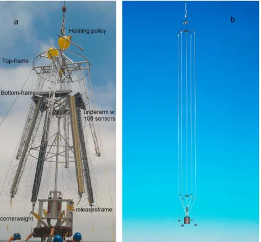
For transportation and handling in port, the entire mooring is fold up (Figure 1a). This 6 m tall, high-grade aluminum structure consists of two sets of four arms 3 m long. We mounted 5 × 95 = 475“NIOZ4” high-resolution temperature (T)-sensors in tubes taped at 1.0 m intervals tofive 104 m long, 0.0032 m diameter thin nylon-coated steel cables. Four cables connect the corner tips of the upper and lower sets of arms; a central instrumented line connects the upper and lower inner frames. After the structure is lifted overboard into the sea by a crane, the arms are unfolded and lines stretched by lowering the central weight. Upon being fully stretched (Figure 1b), the mooring is released into free fall to the seafloor.
The four corner lines are spaced 4.0 m from the central line and 5.6 m between them. Each line is kept under about 1000 N tension distributed from two top buoys totaling 5000 N net buoyancy. This tension and large net buoyancy maintain a relatively stiff mooring, with little motion under current drag. Vertical tilt was small (<1°). Heading information showed commonly <1° variations of compass data around their mean values, except brief<10° variations during three strong (~0.22 m s 1) current speed events. The T-sensors were located between 5 and 99 m above the bottom. They sampled at 1 Hz, with a precision better than 5 × 10 4°C and a noise level of 1 × 10 4°C [van Haren et al., 2009]. Every 4 h, all sensors were synchronized to a single clock via induction. Due to various problems, 33 of the 475 sensors did not function properly. Their data are not considered.
Figure 1. (a) Compacted 3-D mooring array of temperature sensors just before deployment in the ocean. (b) Model of the unfolded array to scale.
This 3-D thermistor array was successfully moored at 37°00′N, 013°48′W, and 1740 m water depth on the eastern flank of Mount Josephine, about 400 km southwest of Lisbon (Portugal) in the NE Atlantic on 2 May 2015 (year-day 121). The line orientation was directed southeast-northwest SE-NW (lines 1 and 4), NE-SW (lines 2 and 3) to within ±5°, with lines 1 and 2 facing downslope (direction ~ESE). The average local bottom slope of about 10° is more than twice as steep (supercritical) than the average slope of internal tides under local stratification condi-tions [van Haren et al., 2015]. The site is also well below the Mediterranean Sea outflow (between 1000 and 1400 m), so that salinity compensated apparent density inversions in temperature are expected to be minimal. The 38 days of T-data are converted into“Conservative” (~potential) Temperature data Θ [IOC, SCOR, IAPSO, 2010]. They are used as a tracer for density anomaly referenced to 1600 m (σ1.6) variations following the relation
δσ1.6=αδΘ, α = 0.044 ± 0.005 kg m 3°C 1for the depth range [1500 2000] m, whereα denotes the apparent
thermal expansion coefficient under local conditions [van Haren et al., 2015]. This relation is established from nearby shipborne Conductivity-Temperature-Depth profile data. The high spatial (1 m in the vertical) and tem-poral (1 Hz) resolution of the T-sensors, in combination with their low noise level, allows the estimation of the vertical averages of the dissipation rate of turbulent kinetic energy< ε > and vertical eddy diffusivity < Kz> via
reordering [Thorpe, 1977]. Vertical averaging is denoted by <>. Although this method has been used frequently in the past, mostly from shipborne or free-fall profiling data, its assumptions have been debated from recent numerical studies [e.g., Chalamalla and Sarkar, 2015; Mater et al., 2015]. The latter study shows that instantaneous dissipation rates estimated from this method may be biased high by a factor of 4 during large convective events but that this bias disappears after sufficient geometrical averaging. In the averaged ε and Kzvalues reported below this bias is thus minimized (well within one standard deviation of error). Based on
pre-vious detailed analyses using data from a similar 100 m long but 1-D mooring nearby [Cimatoribus and van Haren, 2015, 2016], we can confidently say that while convection is an important process, in particular in some parts of the water column and during the upslope tidal phase, shear-driven turbulence is still the dominant process. This is because above such sloping topography internal waves breaking is observed to be a complex mix of convective and shear-driven overturning over a wide range of scales.
Figure 2. High-resolution Conservative Temperature observations at the central line. (a) Entire 38 day time series, a mean from upper (1641 m), middle (1688 m), and lower (1735 m) sensors. The periods of Figures 2b and 2c are indicated by blue bars. (b) Four day period of relatively low tide amplitudes. (c) As in Figure 2b but for large tide amplitudes. The purple line indicates a period with average turbulence levels, detailed in Figure 3.
3. Observations
The main periodicity of internal waves above Mount Josephine is the semidiurnal lunar tide (see temperature sensor data from the central line, Figure 2). The tidal excursion well exceeds the 94 m range of thermistors as none of the color contours can be followed uninterruptedly. This is observed during both a relatively weak tide period (Figure 2b) and one with approximately twice the amplitude (Figure 2c). As usual above sloping topography, fronts representing nonlinear bores and high-frequency internal waves are present, with the sharper fronts when tides are larger (Figure 2c).
The vertically averaged turbulence parameter estimate values of the 1 Hz data have a range of about four orders of magnitude. Mean values are relatively high. Over the displayed 4 days, 94 m full range of sensors and thus not necessarily representing a particular overturn scale, means are as follows: [<ε>] = 1.3 ± 1 × 10 7m2s 3, [<Kz>] = 1.6 ± 1.2 × 10 2m2s 1, and [<N>] = 1.6 ± 0.4 × 10 3s 1 for Figure 2b and [<ε>] = 6 ± 4 × 10 7m2s 3, [<Kz>] = 2.5 ± 1.5 × 10 2m2s 1, and [<N>] = 1.9 ± 0.4 × 10 3s 1for Figure 2c, where [] denotes averaging with time and the error one standard deviation. These mean turbulence levels are more than two orders of magni-tude larger than the canonical value of Kz= 10 4m2s 1 required to maintain the ocean stratified [Munk,
1966]. They are, within error, equal to the largest values observed above Mount Josephine previously, in 350 m deeper waters [van Haren et al., 2015]. They are three orders of magnitude larger than values observed in the ocean interior [e.g., Gregg, 1989].
An example of 600 s time-depth series showing a passage of fronts when turbulence levels are average is given in Figure 3. It shows that incoherent motions can be studied in some detail between thefive lines. These (upslope propagating) fronts are seen tofirst hit at line 1 then 2, c(entral), and lines 3 and 4, the latter about simultaneously. This is more or less visible in the same order for the off-bottom cool front at 1720 m, day 141.4547, the near-bottom cold front at 1735 m, day 141.4575, and the warm depression at 1660 m, day 141.458. Noting that the time-tick marks are at 86 s, typical relative delays are 10–20 s over 4–8 m, yielding
Figure 3. Ten minute detail of data at the purple line in Figure 2, here in thefirst panel labeled “c” for central line. Black contour lines are drawn every 0.05°C. The other panels show the Conservative Temperature observations for the same time window from the four corner lines, labeled 1–4. The black contours are repeated from the first panel (central line).
an estimate of phase/propagation speed of 0.4 m s 1. This is about twice the particle/current speed measured by a large-scale acous-tic Doppler current profiler on a simultaneous mooring 1 km away. The turbulence is found at fre-quencies (σ) well beyond the 100 m based (large-scale), buoy-ancy frequency N and the maxi-mum 2 m based (small-scale) buoyancy frequency Ns,max. Two
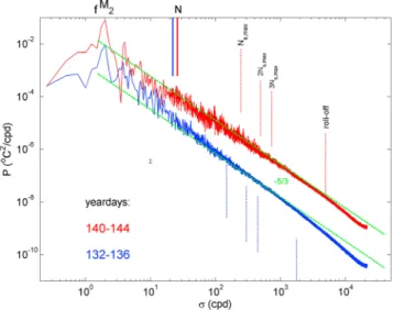
power spectra P, obtained by aver-aging all sensors over a 4 day per-iod (Figure 4), demonstrate an image of the internal wave and turbulence band obtained from 442 independent temperature records in an ocean water column with a volume of 3000 m3. The average spectra show that even at the highest frequency (the Nyquist frequency), the sensors respond above their noise level. There, the width of spectral variation is small, due to the large number of degrees of freedom (~15,000).
For lower frequenciesσ ~ < 3Ns,max, however, this width of variation increases, in particular forσ < 2Ns,max,
evi-dencing larger contributions from coherent signals. Between N< σ < 1000 and 2000 cpd (cycle(s) per day) we expect this to be the turbulence inertial subrange. Roughly, this part of the spectrum follows a slope ofσ 5/3 (green dashed line), particularly for the red spectrum. A 5/3 slope is expected for temperature in a turbulence inertial subrange [Tennekes and Lumley, 1972] or a passive scalar under isotropic conditions [Warhaft, 2000]. Regularly, peaks, like around Ns,max, significantly extend above the inertial subrange background.
The two spectra from weak (blue) and strong (red) tides are not offset deliberately. Their difference in energy is approximately a factor of 4 in the internal wave band f< σ < N, f the inertial frequency, and a factor of about 42= 16 forσ > N. To within error, a factor of 4 is the ratio of the calculated mean dissipation rates and the ratio of the tidal amplitudes squared. With less energy in the blue spectrum, its inertial subrange peaks are smaller and shifted to lower frequencies consistent with smaller buoyancy frequencies. In contrast, the internal wave band is relatively more energetic and its slope is steeper than 5/3 at low frequencies consistent with previous observations under relatively weak turbulent conditions [Cimatoribus and van Haren, 2015].
The all-sensors, 4 day average coherence spectra are given in Figure 5. As expected, the coherence in the range [0.11 0.99] decreases at any frequency with increasing separation distance, both in the vertical (Δz) and in the horizontal (Δx,y). The lower tidal energy period (Figure 5a) shows smaller coherence at all levels and intervals compared with the more energetic period (Figure 5b). For Δz = 1 m during the more energetic period, the coherenceflattens to a low level at about 5000 cpd from lower frequencies. This 5000 cpd corresponds to the roll-off of the red power spectrum in Figure 4. At the high-frequency end (1000–2000 cpd) the observed inertial subrange drops into noise for a vertical separation distance of 2–3 m. Like in the power spectra, several coherence peaks occur within the inertial subrange, foremost for the tidally energetic period (Figure 5b). They coincide in frequency with the power spectral peaks extending above theσ 5/3slope and up to aσ 2slope from the M2peak (as does, e.g., the peak aroundσ = Ns,maxin
Figure 5b). This implies approximately the same energy level in vertical motions at tidal frequencies and at coherent inertial subrange peak frequencies. These inertial subrange peaks are consistent throughout the coherence spectra, independently of the separation distance. They are least well visible for 1 m separation distance, due to its highest coherence.
Figure 4. Temperature power spectra, averages of 442 near-raw periodograms for the Kaiser window tapered time series of the 4 day periods in Figures 2b (blue) and 2c (red). The data are subsampled at 0.5 Hz for computational reasons. Besides inertial (f) and semidiurnal lunar tidal (M2) frequencies several
buoyancy frequencies are indicated including 4 day large-scale mean N and the maximum small-scale Ns,max. The value 5/3 indicates the spectral slopeσ 5/3.
The 95% significance level is indicated by the small vertical bar.
Comparing the vertical and horizontal coherence spectra demonstrates the transition from anisotropy to isotropy through the inertial subrange. At the high-frequency end of the internal wave band,σ = N, the coher-ence level of horizontal separation distanceΔx,y = 4 m coincides with that of vertical Δz = 1–2 m, while Δx, y = 8 m coincides with that ofΔz = 2–4 m. This suggests an anisotropic aspect ratio of 0.25–0.5, depending on the tidal energy. When the frequency increases, this aspect ratio becomes equal to 1 near 2Ns,max, as
Δx,y = 4 m (Δx,y = 8 m) nearly match that of Δz = 4 m (Δz = 8 m). Below this cutoff, the coherence drops below the 95% significance level. The coherence measurements hence capture the transition from anisotropy to isotropy of theflow in a much clearer way than the power spectrum, although in the latter the σ 5/3slope is permanently reached for approximately 2Ns,max< σ (<270 N).
4. Discussion
Ocean flows commonly create environments with high bulk Reynolds numbers (Re = UL/ν), with values reaching Re = O(104–106) in areas where internal wave breaking is imminent such as the one studied here. Parameters used for this scaling are, U = O(0.01–0.1) m s 1, the velocity scale, L = O(1–10) m, the length scale, and,ν = 10 6m2s 1, the kinematic viscosity. In spite of the relatively large turbulence levels generated by such wave breaking, the ocean rapidly restratifies in stable density layers. The present observations shed some light on the anisotropic nature of stratified turbulence in such a deep-sea environment. Hereby, the small-scale density layering plays an important role in determining the scale of separation between anisotro-pic (lower frequencies) and isotroanisotro-pic (higher frequencies) motions. This study suggests that this separation occurs at about twice the small-scale buoyancy frequency. This resembles thefindings by Gargett [1988], here for higher Reynolds numberflows. The frequencies at which isotropy is found likely relate with Froude num-ber equal to 1 [Billant and Chomaz, 2001]. Unfortunately, we lacked adequate local current measurements to verify this.
The results presented in this study are unique following years of attempts in performing three-dimensional measurements of oceanic turbulence. To our knowledge, these data are thefirst observational evidence of the transition from anisotropy to isotropy in geophysical turbulence. Thus far, coherence computations separated internal wave from turbulent motions at the large-scale buoyancy frequency N [e.g., Briscoe, 1975], without further detailing the inertial subrange as in the present data. The transition frequency
Figure 5. Average coherence spectra between all pairs of independent sensors for the labeled vertical (Δz) and horizontal (Δx,y) distances. The low dashed lines indicate the approximate 95% significance levels computed following Bendat and Piersol [1986]. (a) Weak tide period of Figure 2b. (b) Strong tide period of Figure 2c.
between anisotropic and isotropic turbulence of about 2Ns,maxobserved here informs about the particular scale of motions at the separation. This separation is found at frequencies well beyond N and is related to the small-scale stratification. This stresses the larger importance of the formation of (thin) layering than large-scale stratification for anisotropy. Perhaps, the observed inertial subrange peak frequencies indicate an interaction between this small-scale layering and the larger-scale near-inertial and tidal internal wave motions, but this requires further study.
The present array offive 100 m long lines 4 and 5.6 m apart seems an upper limit for the size of mooring to be deployed in one action. For larger scales and more lines other solutions have to be found. One could lower mooring lines via a winch cable several thousands of meters all the way to the bottom. Hereby, a precision of a few meters horizontally can only be obtained using a short-baseline system to be deployedfirst. This is an elaborate additional operation, performed only for an extensive set of moorings such as the ANTARES under-water neutrino telescope off Toulon, France [Ageron et al., 2011]. However, the present ANTARES mooring line separation is 90 m on average, which exceeds the required horizontal decorrelation scale resolution for internal waves by one order of magnitude [Briscoe, 1975; LeBlond and Mysak, 1978] and which narrowed to 4 m here.
References
Ageron, M., et al. (2011), ANTARES: Thefirst undersea neutrino telescope, Nucl. Instrum. Methods Phys. Res., Sect. A, 656, 11–38. Aghsaee, P., L. Boegman, and K. G. Lamb (2010), Breaking of shoaling internal solitary waves, J. Fluid Mech., 659, 289–317. Bendat, J. S., and A. G. Piersol (1986), Random Data: Analysis and Measurement Procedures, 566 pp., Wiley, New York. Billant, P., and J.-M. Chomaz (2001), Self-similarity of strongly stratified inviscid flows, Phys. Fluids, 13, 1645–1651.
Briscoe, M. G. (1975), Preliminary results from the trimoored internal wave experiment (IWEX), J. Geophys. Res., 80, 3872–3884, doi:10.1029/ JC080i027p03872.
Chalamalla, V. K., and S. Sarkar (2015), Mixing, dissipation rate, and their overturn-based estimates in a near-bottom turbulentflow driven by internal tides, J. Phys. Oceanogr., 45, 1969–1987.
Cimatoribus, A. A., and H. van Haren (2015), Temperature statistics above a deep-ocean sloping boundary, J. Fluid Mech., 775, 415–435. Cimatoribus, A. A., and H. van Haren (2016), Estimates of the temperatureflux-temperature gradient relation above a sea-floor, J. Fluid Mech.,
793, 504–523.
Gargett, A. E. (1988), The scaling of turbulence in the presence of stable stratification, J. Geophys. Res., 93, 5021–5036, doi:10.1029/ JC093iC05p05021.
Gregg, M. C. (1989), Scaling turbulent dissipation in the thermocline, J. Geophys. Res., 94, 9686–9698, doi:10.1029/JC094iC07p09686. IOC, SCOR, IAPSO (2010), The international thermodynamic equation of seawater—2010: Calculation and use of thermodynamic properties
Intergovernmental Oceanographic Commission, Manuals and Guides No. 56, 196 pp., UNESCO, Paris, Fr. LeBlond, P. H., and L. A. Mysak (1978), Waves in the Ocean, 602 pp., Elsevier, New York.
Mater, B. D., S. K. Venayagamoorthy, L. S. Laurent, and J. N. Moum (2015), Biases in Thorpe scale estimates of turbulence dissipation. Part I: Assessments from large-scale overturns in oceanographic data, J. Phys. Oceanogr., 45, 2497–2521.
Munk, W. (1966), Abyssal recipes, Deep-Sea Res., 13, 707–730.
Saunders, P. M. (1983), Benthic observations on the Madeira abyssal plain: Currents and dispersion, J. Phys. Oceanogr., 13, 1416–1429. Tennekes, H., and J. L. Lumley (1972), A First Course in Turbulence, 300 pp., MIT Press, Cambridge.
Thorpe, S. A. (1977), Turbulence and mixing in a Scottish loch, Phil. Trans. R. Soc., London A, 286, 125–181.
Thorpe, S. A. (1987), Transitional phenomena and the development of turbulence in stratified fluids: A review, J. Geophys. Res., 92, 5231–5248, doi:10.1029/JC092iC05p05231.
van Haren, H. (2007), Echo intensity data as a directional antenna for observing processes above sloping ocean bottoms, Ocean Dyn., 57, 135–149.
van Haren, H., and L. Gostiaux (2012), Detailed internal wave mixing observed above a deep-ocean slope, J. Mar. Res., 70, 173–197. van Haren, H., M. Laan, D.-J. Buijsman, L. Gostiaux, M. G. Smit, and E. Keijzer (2009), NIOZ3: Independent temperature sensors sampling
yearlong data at a rate of 1 Hz, IEEE J. Ocean. Eng., 34, 315–322.
van Haren, H., A. Cimatoribus, and L. Gostiaux (2015), Where large deep-ocean waves break, Geophys. Res. Lett., 42, 2351–2357, doi:10.1002/ 2015GL063329.
Warhaft, Z. (2000), Passive scalars in turbulentflows, Annu. Rev. Fluid Mech., 32, 203–240.
Geophysical Research Letters
10.1002/2016GL068032
Acknowledgments
This research was supported in part by NWO, the Netherlands Organization for the advancement of science. L.G. is supported by the Agence Nationale de la Recherche, ANR-13-JS09-0004-01 (STRATIMIX). We thank the captain and crew of the R/V Pelagia and NIOZ-MTM for their very helpful assistance during deployment and recovery. We thank J. van Heerwaarden, R. Bakker, and M. Laan for all the work, discussions, and trials during design and construction. Data use requests can be directed to hans.van.haren@nioz.nl.