HAL Id: hal-01821922
https://hal.umontpellier.fr/hal-01821922
Submitted on 23 Jun 2018
HAL is a multi-disciplinary open access
archive for the deposit and dissemination of sci-entific research documents, whether they are
pub-L’archive ouverte pluridisciplinaire HAL, est destinée au dépôt et à la diffusion de documents scientifiques de niveau recherche, publiés ou non,
Quantifying Variation in Speciation and Extinction
Rates With Clade Data
Emmanuel Paradis, Pablo Tedesco, Bernard Hugueny
To cite this version:
Emmanuel Paradis, Pablo Tedesco, Bernard Hugueny. Quantifying Variation in Speciation and Ex-tinction Rates With Clade Data. Evolution - International Journal of Organic Evolution, Wiley, 2013, 67 (12), pp.3617 - 3627. �10.1111/evo.12256�. �hal-01821922�
Running head: VARIATION IN SPECIATION AND EXTINCTION
QUANTIFYING VARIATION IN SPECIATION AND
EXTINCTION RATES WITH CLADE DATA
Emmanuel Paradis1,3, Pablo A. Tedesco2 and Bernard Hugueny2
1Institut de Recherche pour le D´eveloppement, ISEM UMR 226/5554 – UM2/CNRS/IRD,
Jl. Taman Kemang 32B, Jakarta 12730, Indonesia
2UMR Biologie des ORganismes et des ´Ecosyst`emes Aquatiques (UMR BOREA, IRD
207-CNRS 7208-UPMC-MNHN), D´epartement Milieux et Peuplements Aquatiques,
Mus´eum National d’Histoire Naturelle, 43 rue Cuvier, 75231 Paris cedex, France 3Email: [email protected]
High-level phylogenies are very common in evolutionary analyses, though they are
of-1
ten treated as incomplete data. Here we provide statistical tools to analyze what we
2
name ‘clade data’, that are the ages of clades together with their numbers of species.
3
We develop a general approach for the statistical modeling of variation in speciation
4
and extinction rates, including temporal variation, unknown variation, and linear and
5
nonlinear modeling. We show how this approach can be generalized to a wide range of
6
situations, including testing the effects of life-history traits and environmental variables
7
on diversification rates. We report the results of an extensive simulation study to assess
8
the performance of some statistical tests presented here as well as of the estimators of
9
speciation and extinction rates. These latter results suggest the possibility to estimate
10
correctly extinction rate in the absence of fossils. An example with data on fish is
11
presented.
12
KEY WORDS: birth–death models, extinction, maximum likelihood, speciation, stem
13
ages.
The study of the tempo and mode of evolution has experienced a new wave 15
of interest from evolutionists using new mathematical and statistical tools 16
to analyze molecular phylogenies (Sanderson and Donoghue 1996; Ricklefs 17
2007). Following some initial breakthrough (e.g., Nee et al. 1992, 1994), sig-18
nificant progress has been achieved in biologically relevant statistical mod-19
eling of diversification, such as quantifying temporal variation in diversifi-20
cation (Paradis 2011; Hallinan 2012) or assessing the effects of biological 21
traits on speciation and extinction rates (Maddison et al. 2007; FitzJohn 22
et al. 2009; FitzJohn 2010). Recent advances have also been accomplished 23
in integrating molecular and fossil data (e.g., Morlon et al. 2011; Didier et al. 24
2012). 25
Most of these recent statistical developments have focused on analyz-26
ing complete phylogenies. Incomplete phylogenies are often treated as a 27
seperate case in order to take missing data into account (Pybus et al. 2002; 28
FitzJohn et al. 2009; Stadler 2011). The most common form of such data is 29
a phylogeny resolved at a high level accompanied by the number of species 30
associated to each tip of the tree. On the other hand, the ages of clades 31
together with the numbers of species (named here ‘clade data’) have been 32
a neglected source of data in the analysis of diversification. Magall´on and 33
Sanderson (2001) provided some methods for the analysis of such data and 34
applied them to angiosperms. They particularly developed various estima-35
tors of the (net) rate of diversification of a clade giving its age and number 36
of species. 37
The relative lack of interest towards clade data may come from the fact 38
that, for a given clade, its complete phylogeny contains more information 39
than the pair of values ‘age + number of species’. However, for a collection 40
of clades, such data are a valuable source of information for several reasons. 41
First, clades defined by higher-level taxa (e.g., families, orders) are clearly 42
identified for almost all groups of living beings and their numbers of species 43
are in many cases already known. Second, phylogenetic relationships among 44
higher-level taxa have been much more studied than within them, so it is 45
more straightforward to date the age of a clade rather than the divergences 46
among its species. Third, the fossil record is generally more informative on 47
the origin of higher-level taxa compared to species or other low-level taxa. 48
Fourth, it is easier to examine the impact of the species concept on the 49
definition of clade data rather than on a phylogeny since, in the former the 50
species concept will mostly affect the number of species while in the latter it 51
will be often hard to infer different phylogenies under those distinct species 52
definitions. Clade data have also some disadvantages: the inherent lack 53
of temporal resolution within each clade makes it impossible to study the 54
variation in diversification within them. 55
In the present paper, we extend the approach presented by Magall´on
56
and Sanderson (2001) and present statistical tools for the inference of di-57
versification patterns and processes with clade data. Our approach assumes 58
that each clade, instead of having its own speciation and extinction rates, 59
comes from a ‘statistical population of clades’ so that maximum likelihood 60
inference is straightforward. With this rationale, we show how to make 61
inference on variation in diversification parameters among clades using dif-62
ferent modeling tools, including testing the effects of life-history traits and 63
environmental variables and the case where variation is a priori unknown. 64
We also present the results of a simulation study in order to assess the sta-65
tistical performance of several tests and estimators presented in this paper, 66
and finally we apply our approach on a data set of fish. 67
Statistical Modeling Approach
68
Throughout this paper we assume that diversification proceeds with speci-69
ation (λ) and extinction (µ) rates which are the probabilities that a species 70
splits into two daughter-species or goes extinct during a very short time. 71
We denote as Xt the number of species in a clade of age t where this may
72
be either the stem age of the clade (divergence time of the clade from its 73
sister-clade) or its crown age (time to the most common recent ancestor 74
of the species belonging to the clade). Specifically, using equation 8 from 75
Kendall (1948), we can write the probability that Xttakes a specific integer
76
value x: 77
Pr(Xt= x|θ, X0= 1) = ηt(1 − ηt)x−1 x ≥ 1, (1)
where θ is a vector of parameters specifying how speciation and extinction 78
rates vary through time and ηt is a function of these parameters. The
79
conditioning on X0 = 1 emphasizes that in this paper we consider stem
80
groups. For the case of crown groups (X0 = 2), the probabilities must
81
be summed on all possible combinations. In most applications, stem groups 82
are considered because the origin of a group is inferred from its relationships 83
with its sister-group. On the other hand, deriving the crown age of a group 84
requires to estimate the age of the most recent common ancestor of its species 85
which is usually more complicated because it requires to sample all species 86
in the clade. On the other, inferring stem ages requires one species from the 87
clade and one from its sister-clade. 88
Various forms exist for these probabilities depending on the parameteri-89
zation of θ and whether we wish to condition them on survival of the lineage 90
until present or not. For instance, if extinction rate is zero and speciation 91
rate is constant, then ηt= e−λt. This is the Yule (1924) model. Models with
a non-null extinction rate are called birth–death models (Kendall 1948). 93
The point of conditioning on no extinction is important when analyzing 94
data on actual groups because total extinction of these groups did not occur. 95
Thus the probabilities must be modified accordingly, otherwise this would 96
result in underestimated extinction rates (Rabosky et al. 2007). 97
Let us consider for the moment the simple Yule model. The expected 98
number of species at time t is given by E(Xt) = eλt. From this expectation,
99
a simple estimator of λ based on the method of moments is ˆλ = ln(x)/t
100
(Magall´on and Sanderson 2001). When considering a single clade, and in
101
the absence of more detailed information, it does not seem possible to go 102
further in the inference. When considering more than one group (e.g., the 103
families within an order or a class), researchers usually estimate λ separately 104
for each group, then proceed with standard statistics (e.g., McPeek 2008). 105
This approach assumes that each clade is characterized by its own speciation 106
rate. On the other extreme, one may assume that speciation rate is the same 107
in all groups so that the observed data are independent outcomes of the 108
same diversification process. Thus, it is possible to use maximum likelihood 109
inference using equation 1. The likelihood function is: 110
Y
i
Pr(xi|λ), (2)
where Pr(x|λ) is a simplified notation of equation 1. We may expect less 111
bias in the estimates from this approach, but also the possibility to test 112
hypotheses based on fitting alternative models. 113
The assumption of equal speciation rates among clades is, certainly in 114
most cases, unrealistic (Purvis et al. 1995; Paradis 2005; Alfaro et al. 2009). 115
However, since we have several observations we may model the variation 116
such approaches below. Firstly, we consider approaches based on determin-118
istic variation between two or more groups of clades. Secondly, we consider 119
how temporal variation in speciation and extinction rates can be modeled 120
and assessed. Thirdly, we develop an approach handling unknown variation 121
based on mixture modeling, including the combination of mixtures with a 122
linear modeling of the speciation rate. Finally, we attack the problem of 123
estimating extinction rates. 124
Variation Among Clades 125
A simple way to model variation in diversification among clades is to assume 126
that there are two categories: some clades diversify with speciation rate λ1
127
and the others with rate λ2. The data are made of n1 and n2 clades in each
128
category, respectively. The likelihood function is: 129 n1 Y i1=1 Pr(xi1|λ1) n2 Y i2=1 Pr(xi2|λ2).
Note that each clade is assigned to a category a priori, although there is 130
no assumption on whether λ1 is greater, or smaller, than λ2. The null
131
hypothesis λ1 = λ2 can be tested by fitting this model and the null model
132
whose likelihood is given by equation 2: the likelihood-ratio test (LRT) 133
comparing these two models follows a χ2 distribution with df = 1. An
134
alternative is to use the Akaike information criterion (Akaike 1973). 135
The present approach is easily generalized to more than two categories: 136
let us denote the number of categories as K, then the likelihood function 137
would become the product of K products: 138 K Y j=1 nj Y ij=1 Pr(xij|λj),
where nj is the number of clades in the jth category. The LRT comparing
139
this model with the null model of homogeneous diversification follows a χ2 140
with df = K − 1. 141
These models assume, mostly for simplicity, that there is no extinction 142
(µ = 0); however, variation in extinction rate can be incorporated in a 143
straightforward way. For instance a model with two categories diversify-144
ing with the same λ but with different extinction rates has the following 145 likelihood function: 146 n1 Y Pr(xi1|λ, µ1) n2 Y Pr(xi2|λ, µ2),
which could be compared with the null model with µ > 0 whose likelihood 147 is: 148 N Y Pr(xi|λ, µ),
with N = n1 + n2. This test is related, but not identical, to the tests
149
of equal diversification using sister-clades where the ages of clades are not 150
needed (Paradis 2012b). 151
The supplementary materials provide annotated R code explaining how 152
to build and fit any model following the present approach. 153
Linear Modeling 154
Following the previous section, two extreme models can be defined: the sim-155
plest one where all clades diversify at the same rate, and the most complex 156
one where each clade has its own parameter(s). This second model will be 157
overparameterized for a likelihood approach. Nevertheless, it is possible to 158
model variation in diversification parameters with linear models. For in-159
stance, we may know a priori some variables that are likely to affect the 160
value of speciation rate (e.g., body size), and a model that relates such ‘co-161
variates’ to speciation rate may be an appropriate candidate to model the 162
variation in diversification among clades. We use here a standard strategy 163
to model variation in a rate with respect to a covariate z: 164
g(λi) = βzi+ α,
where λiis the speciation rate in clade i, g is a function used to transform the
165
rate in order to linearize the relationship, and β and α are two parameters. 166
Here β controls the effect of z on λ: if β > 0 then species with large values 167
of z will speciate faster than those with small values of z (and inversely if 168
β < 0). It is possible to consider more than one predictor in which case 169
the number of parameters is equal to the number of predictors plus one. 170
Nonlinear models can also be considered. Each clade has its own speciation 171
rate given by (with g−1 being the inverse transformation of g): 172
λi = g−1(βzi+ α), (3)
which is used to calculate the likelihood defined by equation 2: the likelihood 173
function is then maximized to estimate β and α (see code in the Supplemen-174
tary Material). A common choice for g is the logit function, ln(λi/(1 − λi)),
175 so g−1 gives: 176 λi= 1 1 + e−(ziβ+α),
The null model is defined by fixing β = 0 in which case λ = 1/(1 + e−α) for 177
all clades. The logit function is well suited for parameters varying between 178
0 and 1 which is the case for speciation rates considered on geological time 179
scales (million of years). However, speciation rates may be larger than one 180
on shorter scales. Other transformations can be used such as the one used 181
below. 182
It must be noted that the variation among clades as modeled in the 183
previous section is a special case of linear models where the membership of 184
a clade to a category is coded with a discrete variable and this variable is 185
entered as a predictor into the linear model after coding it into binary 0/1 186
variable(s) (see appendix in Paradis 2005, for details). Therefore, continuous 187
and categorical predictors can be combined in the linear model. 188
Temporal Variation 189
Kendall (1948) studied the birth–death model in a very general way, in-190
cluding the cases where λ and µ vary through time. Thus it is possible to 191
derive the probability density of the distribution of the xi’s when
diversifi-192
cation changed through time. The likelihood can be defined and fit in the 193
same way as above. Such a temporal model can be compared with the null 194
model of constant diversification with a χ2 test whose df will be equal to 195
the number of additional parameters in the first model. As before, tempo-196
ral variation may reflect speciation and/or extinction rate(s). The simplest 197
temporal model has two rates before and after a given time point in the past, 198
so it has one additional parameter than the null model. Note that if the 199
time point is unknown, it could be estimated from the data so there would 200
be two additional parameters. However, a wide variety of temporal models 201
can be defined in ape (Paradis et al. 2004) using the functiondbdTimewhere 202
the temporal variation is defined by the user with a standard R function. 203
Unknown Variation 204
The above models assume that diversification parameters vary in relation 205
to some known variables, either categorical or continuous. On the other 206
hand, it is possible that these variables are not observable. Such unknown 207
variation can be modeled with two approaches depending on whether we 208
assume that the diversification parameters vary in a discrete or continuous 209
manner. 210
A mixture of distributions is based on the assumption that observations 211
come from two or more categories each characterized by its own distribution, 212
but the assignment of an observation to a particular category is unknown 213
(see Flury et al. 1992, for a biological example). As a simple example,
214
consider a mixture of two Yule processes, then the likelihood function will 215 be: 216 N Y i=1 f Pr(xi|λ1) + (1 − f ) Pr(xi|λ2), (4)
where f is the proportion of clades in the first category. This model has 217
three parameters (λ1, λ2 and f ) and can be compared with the null model
218
of homogeneous speciation with a LRT with df = 2. The idea is easily 219
generalized to more than two mixtures: a mixture with K Yule models 220
would have 2K−1 parameters. As above, the mixture may involve speciation 221
and/or extinction rate(s). By contrast to the situation above where clades 222
were assigned to categories a priori, there is here no assignment a priori. 223
On the other hand, assignment a posteriori is possible by calculating the 224
relative contributions to the likelihood function. 225
The idea may even be further generalized to include mixtures of linear 226
models. Suppose we know that one variable, say body size, has a significant 227
effect on speciation rate but there is some other, unknown, variation in this 228
parameter that we want to model with a mixture. Then it is possible to 229
calculate the λi’s with equation 3 and use them to compute the likelihood
230
with eq. 4. Each category would have its own parameters β and α, so a 231
model with K categories has 3K − 1 parameters. 232
The second approach assumes that, in the case of a Yule model, λ varies 233
continuously across clades following a specified distribution whose parame-234
ters are estimated from the data. A transformation of λ is useful so that it 235
follows a normal distribution: g(λ) ∼ N (µλ, σ2λ). A useful transformation
236
here is the complementary log-log transformation: g(λ) = ln(− ln(λ)). As 237
above we do not know the value of λ for a given clade, but this time instead 238
of a discrete sum we have to do a continuous integration. The likelihood 239 function is thus: 240 N Y i=1 Z ∞ −∞ fN(u|µλ, σλ2) Pr(xi|g−1(u))du,
where fN is the density function of the normal distribution. A graphical
241
representation of the variation in λ is obtained with the inverse transforma-242
tion g−1(u) = exp(−eu) with the dentity of u computed with the normal
243
distribution and the estimates ˆµλ and ˆσ2λ.
244
Estimating Extinction Rates 245
The estimation of extinction rates in the absence of fossil data has appeared 246
to be a complicated issue (Paradis 2004, 2011; McPeek 2008; Aldous et al. 247
2011; Morlon et al. 2011; Didier et al. 2012; Hallinan 2012). To try to tackle 248
this problem, we implemented a procedure which fits a birth–death model 249
estimating λ and µ simultaneously. These estimates are denoted as ˆλBDand
250
ˆ µBD.
Simulation Study
252
The present statistical modeling approach offers many possibilities and it 253
would take a large number of simulations to assess the statistical proper-254
ties of all of them. Instead, we focus on a few key questions. What is the 255
statistical power to detect a difference in diversification between two groups 256
of clades? How powerful is the test to detect temporal variation in diver-257
sification? What is the statistical power to detect unknown variation in 258
diversification between two groups of clades using mixtures? Finally, what 259
is the precision of the λ and µ estimators? 260
To address these four questions, we ran four sets of simulations. First, we 261
considered a simple two-category scenario with n1 and n2 clades simulated
262
with rates λ1 and µ1 and λ2 and µ2, respectively. The times of evolution
263
were drawn from a uniform distribution: ti ∼ U (10, 20). A phylogeny was
264
simulated under a birth–death process during a time ti using ape starting
265
from a single species. The number of species surviving at time ti, xi, was
266
extracted and the pairs (xi, ti) were analyzed as described above using a Yule
267
model. The LRT testing the null hypothesis of homogeneous diversification 268
was computed, and the rejection rate was assessed under different sets of 269
parameter values: n1 = n2= {1, 3, 5, 10, 20}, λ1 = {0.1, 0.15, 0.2}, λ2 = 0.1,
270
µ1= {0, 0.05}, µ2 = {0, 0.05}.
271
Second, we performed simulations under three scenarios with different 272
values of diversification rates before and after 30 time units. We first gen-273
erated 100 values of t from a uniform distribution between 10 and 50. We 274
then simulated clades with constant, increasing, or decreasing diversification 275
rate. The number of species was extracted as before, and two models were 276
fitted: the null Yule model of constant diversification, and an alternative 277
model assuming different speciation rates before and after 30 time units (as 278
above µ = 0 was assumed). The rejection rates of the LRTs comparing both 279
models were computed. 280
Third, a scenario similar to the first one was considered: the difference 281
is that the simulated clades were not identified to a particular category so 282
the data were analyzed with a mixture of Yule models. We used K = 2, 283
n1= n2= {10, 20, 50}, and ti∼ U (10, 20). Four combinations of speciation
284
and extinction rates were used: (i) the null hypothesis is true and there is 285
no extinction: λ1 = λ2 = 0.1, µ1 = µ2 = 0; (ii) the null hypothesis is false
286
and there is no extinction: λ1 = 0.1, λ2 = 0.2, µ1 = µ2 = 0; (iii) the null
287
hypothesis is false but only µ varies: λ1 = λ2 = 0.2, µ1 = 0, µ2 = 0.1; and
288
(iv) same than before with stronger variation in µ: λ1 = λ2 = 0.2, µ1 = 0,
289
µ2= 0.15.
290
Finally, we performed an assessment of the precision of the estimators of 291
speciation and extinction rates using five combinations of λ and µ: (0.1, 0), 292
(0.1, 0.03), (0.1, 0.06), (0.2, 0.1), and (0.2, 0.15). Here ti ∼ U (10, 30) and
293
n = 100. 294
The simulations were replicated 1000 times. Annotated R (R Devel-295
opment Core Team 2012) code is available in the Supplementary Material 296
with guidelines on how to run these simulations so that the readers can 297
adapt them to their own problems. Besides, we did not attempt to compare 298
our method with previous ones because some scenarios considered here can-299
not be analyzed by the latter (e.g., the third scenario does not seem to be 300
tractable with Magall´on and Sanderson’s method).
301
Application to Fish Data
302
We used the data from Vega and Wiens (2012) who compiled the number 303
of species, stem age, and percentage of marine fish species for 22 orders and 304
super-orders and for 97 families. They also provided a phylogeny for the 305
22 higher taxa which allowed to compare our estimates with those obtained 306
from the combined analysis of phylogeny and species richness data (Paradis 307
2003). All data were unmodified from the original publication and are avail-308
able at http://dx.doi.org/10.1098/rspb.2012.0075. With this data set, we 309
explored the variation in diversification using different mixtures of Yule and 310
birth–death models. We also tried to assess whether this variation is due to 311
differences in the speciation or in the extinction rates. 312
Results
313
Simulation Study 314
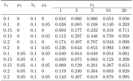
The first set of simulations showed that, overall, the LRT testing for dif-315
ferent diversification rates between two categories of clades had satisfactory 316
statistical properties (Table 1). The type I error rate (rejection rate when 317
the null hypothesis is true, i.e., λ1 = λ2 and µ1 = µ2) was, as expected,
318
close to 5% (first and seventh lines in Table 1). However, when λ − µ was 319
the same in both categories, the rejection rate was greater than 5% (eighth 320
line in Table 1) showing that the present test does not test for equal di-321
versification rate. In the cases where the null hypothesis was not true, the 322
rejection rate varied as expected: it was greater for larger sample sizes (n1)
323
and for larger contrast in the speciation or extinction rate. Interestingly, if 324
one category of clades had smaller µ while λ was the same, then the test was 325
able to detect this difference; however, the statistical power was less than 326
when the same contrast in diversification was due to different λ (compare 327
the second and third lines in Table 1). 328
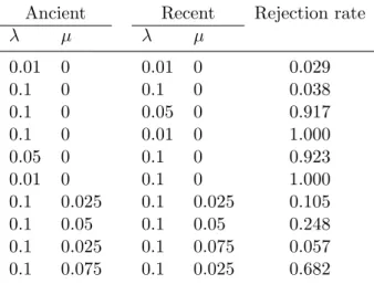
In the second set of simulations, the test for temporal variation rejected 329
the null hypothesis in more than 90% when µ = 0 and λ varied, whether this 330
was an increase or a decrease (third to sixth lines in Table 2). On the other 331
hand, the results were contrasted when µ > 0. When there was no temporal 332
variation in the parameters, the type I error rates were inflated in relation 333
to the value of µ (seventh and eighth lines in Table 2). When µ varied 334
through time, the test behaved very differently depending on the direction 335
of this variation: it did not reject the null hypothesis in most cases when 336
µ increased (nineth line in Table 2) while it rejected it in 68% of the cases 337
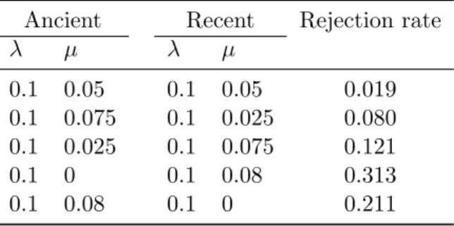
when µ decreased (tenth line in Table 2). To further investigate this point, 338
we repeated some of these simulations but this time the null model was a 339
birth–death model with λ and µ constant through time, and the alternative 340
model was with λ constant and µ allowed to vary before and after 30 time 341
units. In this situation, the test behaved as expected: the rejection rate 342
was less than 5% when µ was constant, whereas it varied between 8% and 343
31% when the null hypothesis was false (Table 3). It is noteworthy that the 344
present test to detect time-dependent extinction rate is not very powerful: it 345
was necessary to simulate a strong contrast in µ to reach a statistical power 346
greater than 0.2. 347
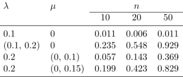
The third set of simulations showed that the mixture-based LRT was 348
able to detect heterogeneous diversification among two unknown categories 349
of clades (Table 4). The test was more powerful when the contrast was 350
due to different λ compared to different µ. Otherwise, the test showed
351
satisfactory statistical performance: its power increased with sample size 352
and/or contrast in the parameters. 353
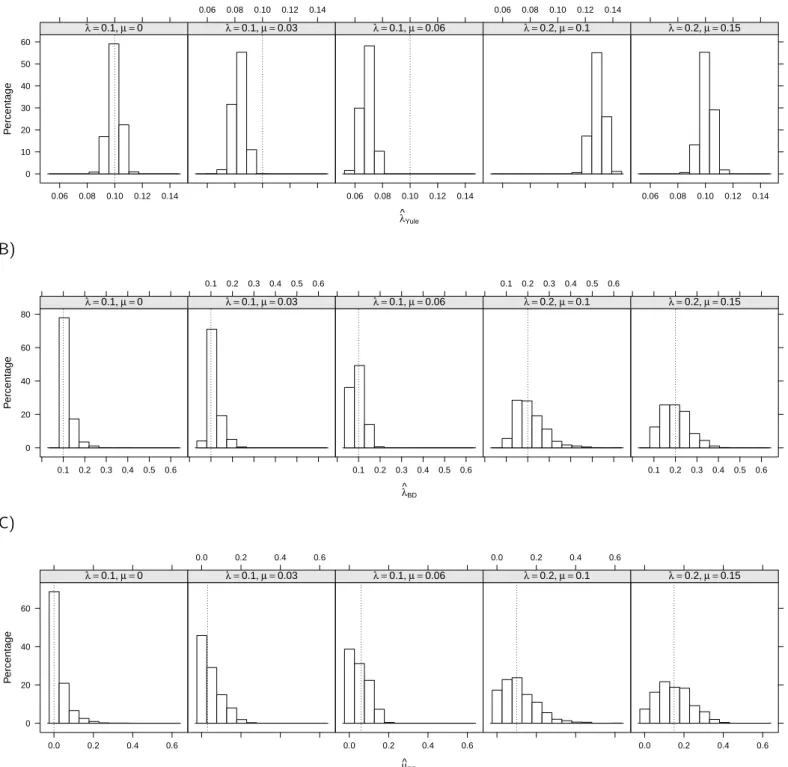
The distribution of the estimates of speciation rate under the Yule model, 354
ˆ
λYule, shows that this estimator appeared unbiased when µ = 0 (Fig. 1A).
355
On the other hand, when µ > 0 it was negatively biased though it can be ob-356
served that ˆλYule> λ − µ so this cannot be actually taken as an estimator of
the net diversification rate. The estimator based on the birth–death model, 358
ˆ
λBD, appears less biased, even though the presence of extinctions seems
359
to induce a slightly more dispersed distribution of the estimates (Fig. 1B). 360
The estimates of extinction rate based on the birth–death model, ˆµBD, were
361
almost unbiased (Fig. 1C). 362
Application to Fish Data 363
The fit of the Yule model to the fish data at the higher level (N = 22) 364
resulted in a global estimate ˆλYule = 0.058 (SE = 0.002; AIC = 456). We
365
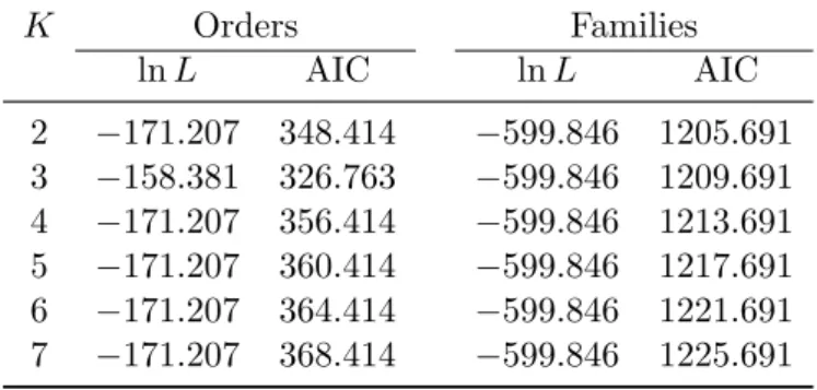
tried to fit a birth–death model which led to a much improved fit (AIC = 366
376); however, the likelihood function had a pronounced ridge on the line 367
λ = µ (not shown). The fit of mixtures of Yule models with increasing 368
number of categories (K) showed that the best fit was with three categories 369
(Table 5). The parameter estimates were: ˆλ1 = 0.041, ˆλ2 = 0.080, ˆλ3 =
370
0.013, ˆf1 = 0.65, and ˆf2 = 0.10. The analysis of the combined taxonomic
371
and phylogenetic data (Paradis 2003) gave ˆλ = 0.056 and ˆµ = 1.83 × 10⁻⁷. 372
The analysis at the level of the families (N = 97) gave for the Yule 373
model ˆλYule = 0.0756 (SE = 0.0016; AIC = 1483). Like above, the fit of
374
the birth–death model resulted in a likelihood surface with a ridge on the 375
line λ = µ. The mixture of Yule models with the best fit had two categories 376
(Table 5); the parameter estimates were: ˆλ1= 0.099, ˆλ2= 0.036, ˆf = 0.42.
377
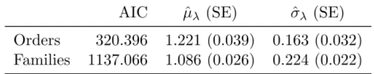
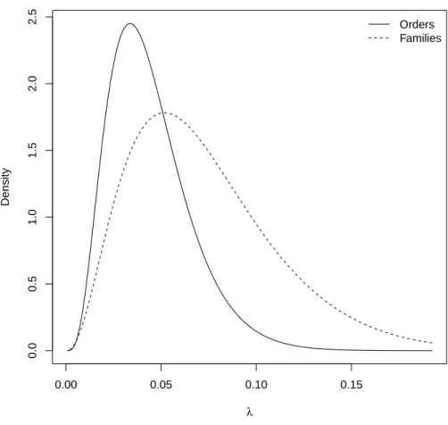
The analysis with a model assuming continuous variation in λ across 378
clades gave close results for both taxonomic levels. In both cases, the model 379
fitted well and the AIC values were smaller than for any of the previous 380
models (Table 6). Figure 2 shows the distribution of λ inferred with the 381
estimated parameters. Trying to introduce µ did not result in successful fits 382
and the estimates of this parameter were close to zero. 383
Vega and Wiens (2012) reported the percentage of marine and freshwater 384
species at both taxonomic levels. This was distributed very asymmetrically 385
with most orders and families having only marine or freshwater species. 386
Thus, we split the data into two groups whether they had more or less 387
than 50% of marine species. A test of different speciation rates between 388
these groups was performed. For orders, the difference was significant (LRT: 389
χ21 = 28.09, P < 0.001) with a larger estimate for marine orders (ˆλ = 0.063, 390
SE = 0.002) compared to the freshwater ones (ˆλ = 0.046, SE = 0.002).
391
An examination of the data suggested that this result was dependent on 392
Percomorpha which is one of the youngest clades in this data set and includes 393
16,625 species (Fig. 3A). Removing this clade resulted in a non-significant 394
test (χ21 = 2.10, P = 0.147, N = 21). For families, an analogous result
395
was found with a significant test (LRT: χ21 = 5.58, P = 0.018) comparing
396
marine families (ˆλ = 0.079, SE = 0.002) and freshwater ones (ˆλ = 0.071, 397
SE = 0.002). This result was dependent on two families older than 200 Myr 398
(Fig. 3B): the Amiidae (one species) and Polypteridae (12). Removing these 399
two families led to a non-significant test: χ2
1 = 2.02, P = 0.155 (N = 95).
400
Discussion
401
The analysis of phylogenetic diversification with molecular data is enjoying 402
a remarkable success in the literature. Some spectacular results have been 403
accomplished using complete phylogenies (e.g., Goldberg et al. 2010; Hugall 404
and Stuart-Fox 2012; Penney et al. 2012). Though complete phylogenies, 405
possibly supplemented with fossil data, are probably the best way to inves-406
tigate evolutionary diversification, the goal of our study was to show the 407
merit of an alternative approach based on the analysis of clade data. 408
Our modeling approach is based on the assumption that each clade is 409
characterized by its diversification parameters and variation among these pa-410
rameters can be quantified in a statistical way. Bokma (2003) and Paradis 411
(2003) developed a method to combine information from high-level phylo-412
genies with clade data: both authors considered the simple constant-rate 413
birth–death model. Alfaro et al. (2009) used similar combined data to as-414
sess variation among clades of vertebrates using a stepwise procedure (see 415
details in Paradis 2012a). Thus the approach in the present paper comple-416
ments previous methodological developments. The possibility to quantify 417
variation among clades with linear models seems a fruitful way to avoid 418
overparameterization. Future applications will reinforce the relative merits 419
of this approach. 420
Recently, Stadler and Bokma (2013) developed alternative likelihood 421
functions with respect to the way higher taxa are defined. They showed 422
that the estimation of speciation and extinction rates vary substantially de-423
pending on these definitions. While they considered only the constant-rate 424
birth–death model, it seems possible and interesting to include their sam-425
pling scheme into the developments presented in the present paper. 426
Our modeling approach ignores the background phylogeny of the clades, 427
the set of branches that link the clades together to make a higher-level 428
phylogeny. There are two reasons for this. First, using information from 429
the background phylogeny is straightforward when the rates of speciation 430
and extinction are constant and homogenous, but when this assumption 431
is relaxed it is not simple how one must assume changes in rates in the 432
background tree. It is clear that if a well-supported background phylogeny 433
is available, this might give additional information which can be combined 434
with clade data (e.g., Paradis 2003). However, this extra information will 435
in most cases require its own model since it relates to older diversification 436
events compared to clade data. On the other hand, ignoring backbone phy-437
logeny and assuming that the clades are independent units simplifies the 438
definition of alternative models as done in this paper. Second, though some 439
higher-level phylogenies are available (mammals, birds), we believe these are 440
still exceptions rather than the rule. For instance, the basal relationships 441
of reptiles, amphibians, or fishes are still debated. Therefore, having the 442
possibility to analyze their clade data without the need of a background 443
phylogeny is of some general application. Furthermore, the present
ap-444
proach can be used when analyzing sets of clades across different phyla, for 445
instance arthropods, echinoderms, vertabrates, etc., where the background 446
phylogeny would not be very informative since this would branch at the 447
origin of Metazoa. 448
The use of mixtures as an approach to analyze heterogeneity in diver-449
sification rates is not limited to clade data. For instance, one could model 450
speciation and extinction rates on a fully-resolved phylogeny assuming that 451
these parameters vary among its branches though we do not know a pri-452
ori which sections of the tree evolved fast and which others evolved slowly. 453
Furthermore, the mixture approach can also be used to model variation in 454
rates of trait evolution along a phylogeny. In that case, the variation may be 455
among branches (as in the previous example), or among traits where some 456
traits are assumed to evolve faster but we do not know which ones. 457
Some subtle but important facts come from the results of the simulation 458
study. Even though most of the tests considered here assumed µ = 0, they 459
appeared not to be tests of equal diversification. If the net diversification 460
rates (λ − µ) were equal among clades, the tests rejected the null hypothesis 461
in more than 5% (see eighth row of Table 1). On the other hand, if λ was 462
equal among clades, the tests detected differences in µ. It is clear that results 463
based only on the Yule model must be interpreted with caution. 464
The tests of temporal variation showed some contrasted but interesting 465
results. When the extinction rate was zero, these tests performed very well 466
and were able to detect either a decrease or an increase in speciation rate. 467
However, when extinction rate was not null, the tests based on the Yule 468
model showed poor performance with an increased type I error rate and a 469
high type II error rate (frequency of accepting the null hypothesis when it is 470
false) when µ decreased through time. These poor performances were cor-471
rected if the assumtion µ = 0 was relaxed (i.e., if a null birth–death model 472
was used in place of the Yule one), though the test had low power. Some 473
of these results make sense: the increased type I error rate obtained with 474
the Yule model is clearly due to the fact that a pattern of accelerated spe-475
ciation can be created under a diversification process with extinction, when 476
old lineages are mostly extinct (e.g., Paradis 2011). On the other hand, the 477
high type II error rate of the same model when extinction rate increased 478
through time is somehow surprising considering the widely reported results 479
of slowing-down diversification (Rabosky and Lovette 2008b,a; Morlon et al. 480
2011; Etienne and Haegeman 2012, among others). Obviously, the same test 481
was not used in these studies, so this clearly requires further investigation. 482
Besides, the result that the test based on a birth–death model shows statis-483
tically consistent results (i.e., the null hypothesis was rejected in less than 484
5% when µ was constant and in more than 5% when this parameter varied 485
through time) is encouraging and will also be further investigated. Interest-486
ingly, this test was more powerful when the extinction rate increased through 487
time. 488
A particularly interesting result comes from the precision of the estimator 489
of extinction rate, ˆµBD, which appears to have a very small bias, even when
the data were simulated with a relatively large value of µ. This contrasts 491
with previous studies showing that the estimator of extinction rate based 492
on complete phylogenies is, overall, inaccurate except if it is small compared 493
to the speciation rate (Paradis 2004; Didier et al. 2012). This result is
494
important because several authors have cast doubt on the possibility to 495
estimate with some precision extinction rates without fossils (Paradis 2011; 496
Aldous et al. 2011). 497
The analysis with the fish data were essentially illustrative, but the re-498
sults call for several comments. The present method seems successful in 499
quantifying variation in diversification rates from a sample of clades. The 500
difference in the results from both taxonomic levels makes sense since we 501
expect more variation among families than among orders. The AIC values 502
evidence that the model assuming continuous variation in λ across clades 503
fits better than a model with discrete variation in this parameter. Since 504
similar tests have not been done with other data, this clearly calls for fur-505
ther analyses before concluding whether diversification varies continuously 506
or discretely across clades. 507
The apparent failure to estimate the extinction rate, µ, of fishes is disap-508
pointing since our simulation study showed that this parameter can be es-509
timated correctly with the present approach. The fossil record shows many 510
episodes of radiations, extinctions, and turn-over during the evolutionary 511
history of fishes (Friedman and Sallan 2012). So the reality is very differ-512
ent from the homogeneous scenario used in our simulations. Our results 513
combined with previous studies (e.g., Aldous et al. 2011) suggest that the 514
estimators of µ are far more complex when rate heterogeneity is present 515
which is likely the case with most real data set. 516
Vega and Wiens (2012) addressed the paradox of equivalent species di-517
versity between marine and freshwater fishes despite the fact that freshwater 518
environments occupy a considerably smaller fraction of the Earth’s surface 519
than oceans. In particular they wondered whether this could be related to 520
differences in diversification rates. Our results are in agreement with these 521
authors’ who tested their hypothesis by correlating the proportion of marine 522
species in a clade with the method-of-moment estimator from Magall´on and
523
Sanderson (2001). We found significant differences in λ between marine and 524
freshwater clades from the raw data; however, the small difference in ˆλ be-525
tween both groups suggested the influence of one or two clades. Hopefully, 526
the analysis of a more comprehensive data set with the statistical tools intro-527
duced in this paper will help to solve the paradox of less biological diversity 528
in the ocean (Mora et al. 2011). 529
Acknowledgments
530
We are grateful to four anonymous reviewers, the Associate Editor, and 531
Laure Kubatko for their constructive comments on previous versions of our 532
manuscript. Financial support was provided by grant ANR-09-PEXT-008. 533
References
534
Akaike, H., 1973. Information theory and an extension of the maximum 535
likelihood principle. Pages 267–281 in B. N. Petrov and F. Csaki, edi-536
tors. Proceedings of the Second International Symposium on Information 537
Theory. Akad´emia Kiado, Budapest.
538
Aldous, D. J., M. A. Krikun, and L. Popovic. 2011. Five statistical questions 539
about the tree of life. Syst. Biol. 60:318–328. 540
Alfaro, M. E., F. Santini, C. Brock, H. Alamillo, A. Dornburg, D. L. Ra-541
bosky, G. Carnevale, and L. J. Harmon. 2009. Nine exceptional radiations 542
plus high turnover explain species diversity in jawed vertebrates. Proc. 543
Natl. Acad. Sci. USA 106:13410–13414. 544
Bokma, F. 2003. Testing for equal rates of cladogenesis in diverse taxa. 545
Evolution 57:2469–2474. 546
Didier, G., M. Royer-Carenzi, and M. Laurin. 2012. The reconstructed 547
evolutionary process with the fossil record. J. Theor. Biol. 315:26–37. 548
Etienne, R. S. and B. Haegeman. 2012. A conceptual and statistical frame-549
work for adaptive radiations with a key role for diversity dependence. Am. 550
Nat. 180:E75–E89. 551
FitzJohn, R. G. 2010. Quantitative traits and diversification. Syst. Biol. 552
59:619–633. 553
FitzJohn, R. G., W. P. Maddison, and S. P. Otto. 2009. Estimating trait-554
dependent speciation and extinction rates from incompletely resolved phy-555
logenies. Syst. Biol. 58:595–611. 556
Flury, B. D., J.-P. Airoldi, and J.-P. Biber. 1992. Gender identification of 557
water pipits (Anthus spinoletta) using mixtures of distributions. J. Theor. 558
Biol. 158:465–480. 559
Friedman, M. and L. C. Sallan. 2012. Five hundred million years of extinc-560
tion and recovery: a Phanerozoic survey of large-scale diversity patterns 561
in fishes. Palaeontology 55:707–742. 562
Goldberg, E. E., J. R. Kohn, R. Lande, K. A. Robertson, S. A. Smith, and 563
B. Igi´c. 2010. Species selection maintains self-incompatibility. Science 564
330:493–495. 565
Hallinan, N. 2012. The generalized time variable reconstructed birth–death 566
process. J. Theor. Biol. 300:265–276. 567
Hugall, A. F. and D. Stuart-Fox. 2012. Accelerated speciation in colour-568
polymorphic birds. Nature 485:631–634. 569
Kendall, D. G. 1948. On the generalized “birth-and-death” process. Ann. 570
Math. Stat. 19:1–15. 571
Maddison, W. P., P. E. Midford, and S. P. Otto. 2007. Estimating a binary 572
character’s effect on speciation and extinction. Syst. Biol. 56:701–710. 573
Magall´on, S. and M. J. Sanderson. 2001. Absolute diversification rates in 574
angiosperm clades. Evolution 55:1762–1780. 575
McPeek, M. A. 2008. The ecological dynamics of clade diversification and 576
community assembly. Am. Nat. 172:E270–E284. 577
Mora, C., D. P. Tittensor, S. Adl, A. G. B. Simpson, and B. Worm. 2011. 578
How many species are there on Earth and in the ocean? PLoS Biol.
579
9:e1001127. 580
Morlon, H., T. L. Parsons, and J. B. Plotkin. 2011. Reconciling molecular 581
phylogenies with the fossil record. Proc. Natl. Acad. Sci. USA 108:16327– 582
16332. 583
Nee, S., R. M. May, and P. H. Harvey. 1994. The reconstructed evolutionary 584
process. Phil. Trans. R. Soc. Lond. B 344:305–311. 585
Nee, S., A. Ø. Mooers, and P. H. Harvey. 1992. Tempo and mode of
586
evolution revealed from molecular phylogenies. Proc. Natl. Acad. Sci. 587
USA 89:8322–8326. 588
Paradis, E. 2003. Analysis of diversification: combining phylogenetic and 589
taxonomic data. Proc. R. Soc. Lond. B 270:2499–2505. 590
Paradis, E. 2004. Can extinction rates be estimated without fossils? J.
591
Theor. Biol. 229:19–30. 592
Paradis, E. 2005. Statistical analysis of diversification with species traits. 593
Evolution 59:1–12. 594
Paradis, E. 2011. Time-dependent speciation and extinction from phyloge-595
nies: a least squares approach. Evolution 65:661–672. 596
Paradis, E. 2012a. Analysis of phylogenetics and evolution with R (second 597
edition). Springer, New York. 598
Paradis, E. 2012b. Shift in diversification in sister-clade comparisons: a 599
more powerful test. Evolution 66:288–295. 600
Paradis, E., J. Claude, and K. Strimmer. 2004. APE: analyses of phyloge-601
netics and evolution in R language. Bioinformatics 20:289–290. 602
Penney, H. D., C. Hassall, J. H. Skevington, K. R. Abbott, and T. N. Sher-603
ratt. 2012. A comparative analysis of the evolution of imperfect mimicry. 604
Nature 483:461–464. 605
Purvis, A., S. Nee, and P. H. Harvey. 1995. Macroevolutionary inferences 606
from primate phylogeny. Proc. R. Soc. Lond. B 260:329–333. 607
Pybus, O. G., A. Rambaut, E. C. Holmes, and P. H. Harvey. 2002. New in-608
ferences from tree shape: numbers of missing taxa and population growth 609
rates. Syst. Biol. 51:881–888. 610
R Development Core Team. 2012. R: a language and environment for
611
statistical computing. R Foundation for Statistical Computing, Vienna. 612
Available at http://www.R-project.org. 613
Rabosky, D. L., S. C. Donnellan, A. L. Talaba, and I. J. Lovette. 2007. 614
Exceptional among-lineage variation in diversification rates during the 615
radiation of Australia’s most diverse vertebrate clade. Proc. R. Soc. Lond. 616
B 274:2915–2923. 617
Rabosky, D. L. and I. J. Lovette. 2008a. Density-dependent diversification 618
in North American wood warblers. Proc. R. Soc. Lond. B 275:2363–2371. 619
Rabosky, D. L. and I. J. Lovette. 2008b. Explosive evolutionary radiations: 620
decreasing speciation or increasing extinction through time? Evolution
621
62:1866–1875. 622
Ricklefs, R. E. 2007. Estimating diversification rates from phylogenetic 623
information. Trends Ecol. Evol. 22:601–610. 624
Sanderson, M. J. and M. J. Donoghue. 1996. Reconstructing shifts in diver-625
sification rates on phylogenetic trees. Trends Ecol. Evol. 11:15–20. 626
Stadler, T. 2011. Mammalian phylogeny reveals recent diversification rate 627
shifts. Proc. Natl. Acad. Sci. USA 108:6187–6192. 628
Stadler, T. and F. Bokma. 2013. Estimating speciation and extinction rates 629
for phylogenies of higher taxa. Syst. Biol. 62:220–230. 630
Vega, G. C. and J. J. Wiens. 2012. Why are there so few fish in the sea? 631
Proc. R. Soc. Lond. B 279:2323–2329. 632
Yule, G. U. 1924. A mathematical theory of evolution, based on the conclu-633
sions of Dr. J. C. Willis, F.R.S. Phil. Trans. R. Soc. Lond. B 213:21–87. 634
Table 1. Rejection rate for the test of equality of diversification rate between two categories with n1and n2 (= n1) clades.
λ1 µ1 λ2 µ2 n1 1 3 5 10 20 0.1 0 0.1 0 0.044 0.060 0.066 0.054 0.056 0.1 0 0.1 0.05 0.038 0.085 0.108 0.140 0.203 0.15 0 0.1 0 0.094 0.177 0.232 0.418 0.711 0.15 0 0.1 0.05 0.112 0.297 0.446 0.759 0.958 0.2 0 0.1 0 0.174 0.497 0.707 0.943 0.998 0.2 0 0.1 0.05 0.236 0.643 0.855 0.993 1.000 0.1 0.05 0.1 0.05 0.040 0.054 0.048 0.054 0.061 0.15 0.05 0.1 0 0.050 0.075 0.083 0.123 0.209 0.15 0.05 0.1 0.05 0.069 0.129 0.201 0.387 0.653 0.2 0.05 0.1 0 0.119 0.240 0.384 0.693 0.928 0.2 0.05 0.1 0.05 0.143 0.407 0.618 0.878 0.995
Table 2. Rejection rate for the test of temporal variation in diversification. The null model was a Yule model with constant rate, and the alternative model was a Yule model with λ allowed to take different values before and after 30 time units. The first two pairs of columns give the parameter values used for the simulations (Ancient and Recent: values before and after 30 time units).
Ancient Recent Rejection rate
λ µ λ µ 0.01 0 0.01 0 0.029 0.1 0 0.1 0 0.038 0.1 0 0.05 0 0.917 0.1 0 0.01 0 1.000 0.05 0 0.1 0 0.923 0.01 0 0.1 0 1.000 0.1 0.025 0.1 0.025 0.105 0.1 0.05 0.1 0.05 0.248 0.1 0.025 0.1 0.075 0.057 0.1 0.075 0.1 0.025 0.682
Table 3. Same than in Table 2 but the null model was a birth–death model with constant rates, and the alternative model was a model with λ constant and µ allowed to take different values before and after 30 time units.
Ancient Recent Rejection rate
λ µ λ µ 0.1 0.05 0.1 0.05 0.019 0.1 0.075 0.1 0.025 0.080 0.1 0.025 0.1 0.075 0.121 0.1 0 0.1 0.08 0.313 0.1 0.08 0.1 0 0.211
Table 4. Rejection rate for the test of equality of diversification rate between two unknown categories using mixtures with n clades in each category.
λ µ n 10 20 50 0.1 0 0.011 0.006 0.011 (0.1, 0.2) 0 0.235 0.548 0.929 0.2 (0, 0.1) 0.057 0.143 0.369 0.2 (0, 0.15) 0.199 0.423 0.829
Table 5. Results of fitting models to the fish data using mixtures of Yule processes with K from two to seven.
K Orders Families ln L AIC ln L AIC 2 −171.207 348.414 −599.846 1205.691 3 −158.381 326.763 −599.846 1209.691 4 −171.207 356.414 −599.846 1213.691 5 −171.207 360.414 −599.846 1217.691 6 −171.207 364.414 −599.846 1221.691 7 −171.207 368.414 −599.846 1225.691
Table 6. Results of fitting a model of continuous variation in speciation rate across orders (N = 22) and families (N = 97) of fish.
AIC µˆλ (SE) σˆλ (SE)
Orders 320.396 1.221 (0.039) 0.163 (0.032)
A) λ^Yule P ercentage 0 10 20 30 40 50 60 0.06 0.08 0.10 0.12 0.14 λ =0.1, µ =0 0.06 0.08 0.10 0.12 0.14 λ =0.1, µ =0.03 0.06 0.08 0.10 0.12 0.14 λ =0.1, µ =0.06 0.06 0.08 0.10 0.12 0.14 λ =0.2, µ =0.1 0.06 0.08 0.10 0.12 0.14 λ =0.2, µ =0.15 B) λ ^ BD P ercentage 0 20 40 60 80 0.1 0.2 0.3 0.4 0.5 0.6 λ =0.1, µ =0 0.1 0.2 0.3 0.4 0.5 0.6 λ =0.1, µ =0.03 0.1 0.2 0.3 0.4 0.5 0.6 λ =0.1, µ =0.06 0.1 0.2 0.3 0.4 0.5 0.6 λ =0.2, µ =0.1 0.1 0.2 0.3 0.4 0.5 0.6 λ =0.2, µ =0.15 C) µ^ BD P ercentage 0 20 40 60 0.0 0.2 0.4 0.6 λ =0.1, µ =0 0.0 0.2 0.4 0.6 λ =0.1, µ =0.03 0.0 0.2 0.4 0.6 λ =0.1, µ =0.06 0.0 0.2 0.4 0.6 λ =0.2, µ =0.1 0.0 0.2 0.4 0.6 λ =0.2, µ =0.15
Figure 1. Distribution of the estimates of λ and µ with (A) the Yule model (ˆλYule) and (B
and C) the birth–death model (ˆλBDand ˆµBD) under five sets of parameters (values are given
0.00 0.05 0.10 0.15 0.0 0.5 1.0 1.5 2.0 2.5 λ Density Orders Families
● ● ● ● ● ● ● ● ● ● ● ● ● ● ● ● ● ● ● ● ● ● 150 200 250 300 1 10 100 1000 10000 Age (Ma) Number of species A) ● ● Freshwater Marine ● ● ● ● ● ● ● ● ● ● ● ● ● ● ● ● ● ● ● ● ● ● ● ● ● ● ● ● ● ● ● ● ● ● ● ● ● ● ● ● ● ● ● ● ● ● ● ● ● ● ● ● ● ● ● ● ● ● ● ● ● ● ● ● ● ● ● ● ● ● ● ● ● ● ● ● ● ● ● ● ● ● ● ● ● ● ● ● ● ● ● ● ● ● ● ● ● 50 100 150 200 250 300 1 5 50 500 Age (Ma) Number of species B)
Figure 3. Number of species with respect to stem clade age for (A) orders and some super-orders and (B) families of fish (the legend is the same for both plots).