HAL Id: hal-01342351
https://hal.inria.fr/hal-01342351
Submitted on 5 Jul 2016
HAL is a multi-disciplinary open access
archive for the deposit and dissemination of
sci-entific research documents, whether they are
pub-lished or not. The documents may come from
teaching and research institutions in France or
abroad, or from public or private research centers.
L’archive ouverte pluridisciplinaire HAL, est
destinée au dépôt et à la diffusion de documents
scientifiques de niveau recherche, publiés ou non,
émanant des établissements d’enseignement et de
recherche français ou étrangers, des laboratoires
publics ou privés.
software product lines
Ganesh Khandu Narwane, José Angel Galindo Duarte, Shankara Narayanan
Krishna, David Benavides, Jean-Vivien Millo, S Ramesh
To cite this version:
Ganesh Khandu Narwane, José Angel Galindo Duarte, Shankara Narayanan Krishna, David
Bena-vides, Jean-Vivien Millo, et al.. Traceability analyses between features and assets in software product
lines. Entropy, MDPI, 2016, 18 (8), pp.269. �10.3390/e18080269�. �hal-01342351�
Article
2
Traceability analyses between features and assets in
3software product lines
4Ganesh Khandu Narwane1,∗, José A. Galindo2,‡,Shankara Narayanan Krishna‡, David
5
Benavides3,‡, Jean-Vivien Millo‡and S Ramesh‡
6
1 Homi Bhabha National Institute, Anushakti Nagar, Mumbai, India; [email protected]
7
2 INRIA, France; [email protected]
8
3 University of Seville, Seville, Spain; [email protected]
9
* Correspondence: [email protected]; Tel.: +91 838 482 0575
10
† Current address: Homi Bhabha National Institute, Anushakti Nagar, Mumbai, India
11
‡ These authors contributed equally to this work.
12
Academic Editor: name 13
Version June 22, 2016 submitted to Entropy; Typeset by LATEX using class file mdpi.cls
14
Abstract: In a Software Product Line (SPL), the central notion of implementability provides the
15
requisite connection between specifications and their implementations, leading to the definition of
16
products. While it appears to be a simple extension of the traceability relation between components
17
and features, it involves several subtle issues that were overlooked in the existing literature. In
18
this paper, we have introduced a precise and formal definition of implementability over a fairly
19
expressive traceability relation. The consequent definition of products in the given SPL naturally
20
entails a set of useful analysis problems that are either refinements of known problems or are
21
completely novel. We also propose a new approach to solve these analysis problems by encoding
22
them as Quantified Boolean Formulae (QBF) and solving them through Quantified Satisfiability
23
(QSAT) solvers. QBF can represent more complex analysis operations, which cannot be represented
24
by using propositional formulae. The methodology scales much better than the SAT-based solutions
25
hinted in the literature and were demonstrated through a tool called SPLAnE (SPL Analysis Engine)
26
on a large set of SPL models.
27
Keywords:Software Product Line, Feature Model, Formal methods, QBF, SAT.
28
1. Introduction
29
Software Product Line Engineering(SPLE) is a software development paradigm supporting joint
30
design of closely related software products in an efficient and cost-effective manner. The starting point
31
of an SPL is the scope, which defines all the possible features of the products in the SPL. The scope is
32
said to define the problem space of the SPL, describing the expectations and objectives of the product
33
line. The description is typically organized as a feature model [1] that expresses the variability of the
34
SPL in terms of relations or constraints (exclusion, requires dependency) between the features and
35
defines all the possible products in the product line.
36
An important step in Software Product Line Engineering (SPLE) is the development of core
37
assets, a collection of reusable artifacts. The core assets contains the components, and we use the
38
term component to represent any artifacts which contributes in products development like code,
39
design, documents, test plan, hardware, etc. A component is an abstract concept of any assets used
40
in products. The core assets, define the solution space of the SPL and are developed to meet the
41
expectations outlined in the problem space [2]. They are developed for systematic reuse across the
42
different products in the SPL [3,4]. The variability in core assets across the components is represented
43
by a component model. The components in a component model, may also have exclude and requires
44
dependency constraints, similarly to feature models.
45
Given the problem and solution spaces for an SPL, as defined by the scope and the core assets,
46
the next important step is traceability, which involves relating the elements (features, core assets) at
47
these two levels [2].
48
The focus of this work is formal modeling and analysis of traceability in an SPL. There are
49
many relationships possible, one of the most useful and natural one is the implementability relation
50
that associates each feature in the scope with a set of core assets that are required for implementing
51
the feature(s) [5]. Beside implementability, many other notions have been defined, thanks to the
52
integration of the variabilities of the problem space and the solution space in the proposed framework.
53
For example, one could be interested in checking whether every product in the problem space has a
54
correspondence in the solution space, i.e., every product represented in the feature model can be
55
implemented using the existing assets considering the implementability relation. Another example is
56
the property to check every asset of an SPL needs to be maintained not only because it is involved in
57
some implementations, but the asset is only option.
58
Let us consider an example from the cloud computing domain. The company offers a service
59
to rent computers on a cloud with different possible software configurations using Linux-based
60
distributions. In the back-end, instead of providing physical machines, the company provides virtual
61
machines with some software package installed on them. Thus, the configuration of machines can be
62
generated on demand according to the needs of the users. In order to improve the speed of creation of
63
a new machine, there are pre-configured machines ready to launch.
64
In this example, the possible configurations offered to the users define the problem space. The
65
set of available Linux packages implementing the features is the core assets. The pre-configured
66
machines can be seen as another set of assets (limited but available immediately).
67
The following are some examples of relevant analyses that could arise in this example:
68
• Check if at least one of the pre-configured machines covers the needs of a new user
69
configuration.
70
• Check if at least one of the pre-configured machines realize (exactly) the needs of a new user
71
configuration.
72
• Check if there are dead packages, i.e. packages that can not be in any of the virtual machines.
73
In the literature, formal modeling and analysis of variability at the feature model level has been
74
studied extensively, and several efficient tools have been built to carry out the analyses [6,7]. The main
75
idea behind all these works is that the variability analysis can be reduced to constraints and variables
76
modeling the feature level variability [2,8–15]. While there are several recent works on traceability,
77
most of them have confined themselves to an informal treatment [16–19]. Some works have chosen a
78
formal approach for representing traceability and configuration of features [20].
79
In the past, most of the work [6,7] has encoded variability analysis operations in propositional
80
formulae [21]. There are various SAT solvers, like SAT4j [22] or MiniSAT [23] or PicoSAT [24], which
81
can be used to check the satisfiability of a propositional formula. We propose a novel approach for
82
modeling traceability and other notions relating features and core assets using Quantified Boolean
83
Formula(QBF) [25]. QBF is a generalization of SAT boolean formulae in which the variables may be
84
universally and existentially quantified. QSAT solver is used to check the satisfiability of Quantified
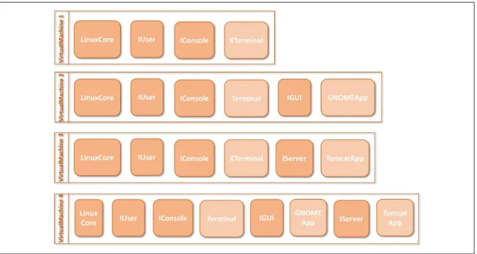
85
Boolean Formula (QBF). In this work, we make use of the well-known QSAT solver, CirQit [26] and
86
RAReQS-NN [27].
87
An early version of this work was published [28]. The proposed method has been implemented
88
in a tool that is integrated with the FaMa framework [29]. This tool, called SPLAnE [30], can model
89
feature models, core assets (component models), and a traceability relations. SPLAnE is a feasible
90
solution for automated analysis of feature models together with assets relations. We believe that
91
this article opens the opportunity for new forms of analysis involving variability models, assets and
92
traceability relations. The following summarizes the contributions of this paper:
• A simple and abstract set-theoretic formal semantics of SPL with variability and traceability
94
constraints are proposed.
95
• A number of new analysis problems, useful for relating the features and core assets in an SPL,
96
are described.
97
• Quantified Boolean Formulae (QBFs) are proposed as a natural and efficient way of modeling
98
these problems. The evidence of scalability of QSAT for the analysis problems in large SPLs
99
(compared to SAT) is also provided.
100
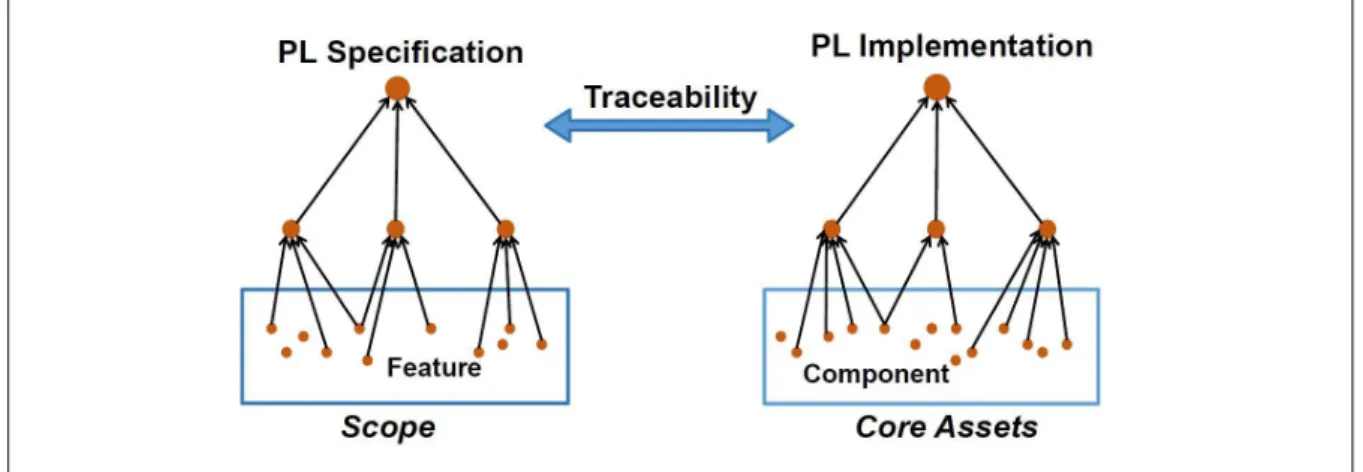
• We present a tool named SPLAnE that enables SPL developers to perform existing operations
101
in the literature over feature diagrams [6] and many new operations proposed in this paper. It
102
also allows to perform analysis operations on a component model and SPL model. We used
103
the FaMa framework to develop SPLAnE that makes it flexible to extend with new analyses of
104
specific needs.
105
• We experimented our approach with numbers of models i.e. i) Real and large debian models, ii)
106
Randomly generated SPL models from ten features to twenty thousand features with different
107
level of cross-tree constraints and iii) SPLOT repository models. The experimental results also
108
gives the comparison across two QSAT solvers (Cirqit and RaReQS) and three SAT solvers (Sat4j,
109
PicoSAT and MiniSAT).
110
• An example from the Cloud computing domain is presented to motivate the practical usefulness
111
of the proposed approach.
112
Paper organization. The remainder of the paper is organized as follows: Section 2 shows a
113
motivating scenario for using SPLAnE ; Section3 presents the tool SPLAnE which is implemented
114
based on proposed approach; Section4describes different analysis operations to extract information
115
by using the SPLAnE tool. Section5analyzes empirical results from experiments that evaluate the
116
scalability of SPLAnE ; Section6 compares our approach with related work; and finally, Section 8 117
presents concluding remarks.
118
2. Motivating example
119
In this paper, we present the cloud computing as a product line. Feature model and component
120
model is used to manage the variability across the scope and core assets respectively.
121
2.1. Feature Models
122
Feature models have been used to describe the variant and common parts of the product line
123
since Kang [31] has defined them. The sets of possible valid combinations of those features are
124
represented by using different constraints among features. The feature model in Figure1represents
125
the features provided by the cloud computing. Two different kinds of relationships are used: i)
126
hierarchical relationships, which describe the options for variation points within the product line; and
127
ii) cross-tree constraints that represent constraints among any features of the feature tree. Different
128
notations have been proposed in the literature [6]; however, most of them share the following
129
relationship flavors:
130
Four different hierarchical relationships are defined:
131
• mandatory: this relationship refers to features that have to be in the product if its parent feature
132
is in the product. Note that a root feature is always mandatory in feature models.
133
• optional: this relationship states that a child feature is an option if its parent feature is included
134
in the product.
135
• alternative: it relates a parent feature and a set of child features. Concretely, it means that
136
exactly one child feature has to be in the product if the parent feature is included.
137
• or: this relationship refers to the selection of at least one feature among a group of child features,
138
having a similar meaning to the logical OR.
139
Later, two kinds of cross-tree relationships are used:
Figure 1.Feature Model: Virtual Machine
• requires: this relationship implies that if the origin feature is in the product, then the destination
141
feature should be included.
142
• excludes: this relationship between two features implies that, only one of the feature can be
143
present in a product.
144
Cloud computing technology provides ready to use infrastructure for the clients. The cloud
145
system reduces the cost of maintaining the hardware and software, and also reduces the time to
146
build the infrastructure on the client side. The client pays only for the hardware and software used
147
based on the duration. The feature model for cloud computing is shown in Figure1. The root feature
148
Virtual Machine is a mandatory feature by default. The mandatory relationship is present between the
149
feature Virtual Machine and UserInter f ace, so the feature UserInter f ace has to be present if feature
150
Virtual Machine is present in the product. The optional relationship is present between the feature
151
Language and VirtualMachine, so it is optional to have feature Language in the products. The feature
152
GU I has alternative relationship with its child features{KDE, GNOME, XFCE}. Hence, if feature
153
GU I is selected in a product, then only one of its child feature has to be present in that product. The
154
feature Server has or relationship with its child features{Tomcat, Glass f ish, Klone}. Hence, if feature
155
Server is selected in a product, then at least one of its child feature has to be present in that product.
156
The feature C++requires the feature C to be present in a product. The presence of feature Tomcat in a
157
product does not allow the feature Klone and vice versa. The client can request for a system with the
158
set of features called a speci f ication. The minimum set of features in the specification should contain
159
features{Virtual Machine, UserInter f ace, Console}as they are mandatory features. We can term this
160
as commonality across all the products of an SPL. The specification F={Virtual Machine, UserInter f ace,
161
Console, GU I, KDE, Langauge, C}is valid for the creation of a virtual machine because it satisfies all
162
the constraints in the feature model. The specification F={Virtual Machine, UserInter f ace, Console,
163
GU I, KDE, Language, C++}is not valid because it contains a feature C++so it is necessary to select
164
feature C.
165
Component Model: Similar to a feature model, same notations can be used to represent
166
variability amongst the components present in core assets of an SPL, we call it a Component
167
Model (CM). The variability amongst the components can also be represented by any other models
168
like the Orthogonal Variability Model (OVM), Varied Feature Diagram (VFD) and Free Feature
169
Diagrams (FFDs) [20,32]. The component model in Figure 2 represents the resources available
170
to create a virtual machine. The cloud computing technology will create a virtual machine that
contains a set of components required to implement the features present in the client speci f ication.
172
Such set of components is called an implementation. The implementation C={LinuxCore, IUser,
173
IConsole, Terminal, ILanguage, C-lang, c-lib }is valid because it satisfies all the constraints on the
174
component model, so a virtual machine can be created with these components. The implementation
175
C={LinuxCore, IUser, IConsole, ILanguage, C-lang, c-lib}is invalid, because the component Terminal
176
or XTerminal or both are required to satisfy the component model constraints.
177
Figure 2.Component Model: Linux Virtual Machine Based System
Figure 3.Preconfigured Virtual Machines
Table1 shows the traceability relation between the features and the components. The entry in
178
the row of feature Glass f ish means the component Glass f ishApp implements the feature Glass f ish.
179
Similarly, the feature Console can be implemented by the set of components:{IConsole, XTerminal} 180
or {IConsole, Terminal}. For each feature in the client specification, the traceability relation gives
181
the required sets of components. In the feature model, the effective features are only the leaf
182
features. The traceability of a parent feature like the feature GU I can be implemented by the set
183
of components: {IGU I}. The feature GU I can be abstracted by eliminating all of its child features
184
{KDE, GNOME, XFCE}; this allows to analyze the SPL at a higher level of abstraction. Section3refer
185
column 3 and 4 from Table1to represent the short name for features and components respectively,
Figure3shows the four preconfigured virtual machines. The preconfigured machines show the
187
set of components from the component model shown in Figure2.
188
Table 1.Traceability Relation for Virtual Machine.
Feature Components Feature Components
Virtual Machine {{LinuxCore}} f1 {{c1}} UserInter f ace {{IUser}} f2 {{c2}}
Language {ILanguage} f8 {{c14}}
Server {{IServer}} f12 {{c10}}
Console {{IConsole, XTerminal}, f3 {{c3, c4},{c3, c5}}
{IConsole, Terminal}} GU I {{IGU I}} f4 {{c6}} KDE {{KDEApp}} f5 {{c7}} GNOME {{GNOMEApp}} f6 {{c8}} XFCE {{XFCEApp}} f7 {{c9}} C {{C-lang, c-lib}} f9 {{c15, c16, c17}} C++ {{C-lang, c-lib, gcc, c++lib}} f10 {{c15, c16, c17, c20}} Java {{OpenJDK},{OracleJDK}} f11 {{c18},{c19}} Tomcat {{TomcatApp}} f13 {{c11}} Glass f ish {{Glass f ishApp}} f14 {{c12}}
Klone {{KloneApp}} f15 {{c13}}
Software product lines can contain a large set of different products. Therefore, facing the
189
complexity of the feature models that represent the products within an SPL is hard. To help in such a
190
difficult task, researchers rely on the computer-aided extraction of information from feature models.
191
This extraction is usually known as the automated analysis in the area. To reason about those models,
192
the relationships existing in the feature model are processed through a CSP, SAT, BDD solver or a
193
specific algorithm. Later, the operation is used to extract specific information from the model. An
194
SPL with twelve leaf features can result in a search space of 212 possible products. Analysis of such
195
a huge search space is a non-trivial task. Some interesting analyses that could performed in this
196
scenario of a Virtual Machine Product Line (VMPL) are as follows:
197
1. Check if at least one of the pre-configured machines covers the needs of a new user
198
configuration: In VMPL, there is always a need to check the existence of any virtual machine
199
as per the given user specification. For example, the specification F={Virtual Machine,
200
UserInter f ace, Console, GU I, GNOME} should be first analyzed to check the existence of
201
any implementation that implements F. The implementation C={LinuxCore, IUser, IConsole,
202
Terminal, IGU I, GNOMEApp, IServer, TomcatApp} (equivalent to preconfigured virtual
203
machine 2 in Figure3) provides all the features in the specification F, it means that there exists
204
a pre-configured machine which covers the user specification F.
205
2. Check if at least one of the pre-configured machines realizes (exactly) the needs of a new user
206
configuration: Multiple implementations may cover a given user specification F. We can analyze
207
the VMPL to find the realized implementation for the user specification. For example, the
208
implementation C={LinuxCore, IUser, IConsole, Terminal, IGU I, GNOMEApp}(equivalent to
209
preconfigured virtual machine 3 in Figure 3) exactly provides all the feature in the specification
210
F.
211
3. Check if there are dead packages: Actual VMPLs contain a huge number of components for
212
Linux systems. The components that are not present in any of the products are termed as dead
213
elements in the product line. In the given VMPL, none of the components is dead.
214
3. SPLAnE framework: Traceability and Implementation
Specification and Implementation
216
The set of all features found in any of the products in a product line defines the scope of the
217
product line. We denote the scope of a product line byF. A scopeF consists of a set of features,
218
denoted by small letters f1, f2. . . . Specifications are subsets of features in the scope and are denoted
219
by F1, F2, . . . , with possible subscripts. On the other hand, the collection of components in the product
220
line defines the core assets and is denoted asC. Small letters c1, c2. . . etc. represent components.
221
Implementations (subsets of components) are denoted by capital letters C1, C2. . . . with possible
222
subscripts. A Product Line (PL) specification is a set of speci f ications in an SPL, denoted asF ∈ ℘( ℘( 223
F )\ {∅}). Similarly, a Product Line (PL) implementation is denoted asC ∈ ℘(℘(C) \ {∅}). In VMPL,
224
the scope, core assets, specifications and implementations are as follows:
225
• Scope F = {f1 : Virtual Machine, f2 : UserInter f ace, f3 : Console, f4 : GU I, f5 : KDE,
226
f6 : GNOME, f7 : XFCE, f8 : Language, f9 : C, f10 : C++, f11 : Java, f12 : Server, f13 : Tomcat,
227
f14: Glass f ish, f15: Klone}
228 229
• Core Assets C = {c1 : LinuxCore, c2 : IUser, c3 : IConsole, c4 : XTerminal, c5 : Terminal,
230
c6 : IGU I, c7 : KDEApp, c8 : GNOMEApp, c9 : XFCEApp, c10 : IServer, c11 : TomcatApp,
231
c12 : Glass f ishApp, c13 : KloneApp, c14 : ILanguage, c15 : C-lang, c16 : c-lib, c17 : gcc,
232
c18: OpenJDK, c19: OracleJDK, c20: c++lib}
233 234
• PL SpecificationF={ 235
F1:{Virtual Machine, UserInter f ace, Console}or{f1, f2, f3},
236
F2:{Virtual Machine, UserInter f ace, Console, GU I, KDE}or{f1, f2, f3, f4, f5},
237
F3:{Virtual Machine, UserInter f ace, Console, Server, Tomcat, Glass f ish}or{f1, f2, f3, f12, f13,
238
f14},
239
F4:{Virtual Machine, UserInter f ace, Console, GU I, KDE, Server, Tomcat}or{f1, f2, f3, f4, f5,
240
f12, f13},
241
F5 :{Virtual Machine, UserInter f ace, Console, GU I, KDE, Language, Java, Server, Tomcat}or
242
{f1, f2, f3, f4, f5, f8, f11, f12, f13}
243
}, where F1, F2, F3, F4and F5are some specifications.
244 245
• PL ImplementationC={ 246
C1:{LinuxCore, IUser, IConsole, XTerminal}or{c1, c2, c3, c4},
247
C2:{LinuxCore, IUser, IConsole, Terminal}or{c1, c2, c3, c5},
248
C3:{LinuxCore, IUser, IConsole, Terminal, IGU I, KDEApp}or{c1, c2, c3, c5, c6, c7},
249
C4 :{LinuxCore, IUser, IConsole, Terminal, IServer, TomcatApp, Glass f ishApp}or{c1, c2, c3,
250
c5, c10, c11, c12},
251
C5:{LinuxCore, IUser, IConsole, Terminal, IGU I, KDEApp, IServer, KloneApp, Glass f ish}or
252
{c1, c2, c3, c5, c6, c7, c10, c12, c13},
253
C6 :{LinuxCore, IUser, IConsole, Terminal, IGU I, KDEApp, IServer, TomcatApp, Glass f ish}
254
or{c1, c2, c3, c5, c6, c7, c10, c11, c12},
255
C7 : {LinuxCore, IUser, IConsole, Terminal, IGU I, KDEApp, ILang, OpenJDK, IServer,
256
TomcatApp}or{c1, c2, c3, c5, c6, c7, c14, c18, c10, c11}
257
}, where C1to C7are some implementations.
258 259
Traceability:
260
We present a formalism for two variation of traceability relation: i) 1: M mapping and ii) N:M
261
mapping. In traceability relation, 1:M mapping is between a feature and a set of component sets, were
262
as N:M is a mapping between feature set and a set of component sets.
263 264
Traceability with 1:M mapping: A feature is implemented using a set of non-empty
265
subset of components in the core asset C. This relationship is modeled by the partial function
266
T : F → ℘(℘(C) \ {∅}). When T (f) = {C1, C2, C3}, we interpret it as the fact that the set of
267
components C1(also, C2and C3) can implement the feature f . WhenT (f)is not defined, it denotes
268
that the feature f does not have any components to implement it.
269 270
Traceability with N:M mapping:A set of features can be implemented using a set of non-empty
271
subset of components in the core assetC. This relationship is modeled by the partial function T :
272
(℘(F ) \ {∅}) → ℘(℘(C) \ {∅}). It may happen that, two features f1and f2can be implemented by
273
a single component c1. In this case,T ({f1, f2}) = {C1}, where C1= {c1}.
274
Definition 1(SPL). An SPL Ψ is defined as a triple hF,C,T i, where F ∈ ℘(℘(F ) \ {∅}) is the PL
275
specification,C ∈ ℘(℘(C) \ {∅})is the PL implementation andT is the traceability relation.
276
The Implements Relation:
277
A feature is implemented by a set of components C, denoted implements(C, f), if C includes a
278
non-empty subset of components C0 such that C0 ∈ T (f). It is obvious from the definition that if
279
T (f) = ∅, then f is not implemented by any set of components. In VMPL, f5 is implemented by
280
implementations C3, C5, C6and C7, but not by implementations C1, C2and C4.
281
In order to extend the definition to specifications and implementations, we define a function
282
Provided_by(C)which computes all the features that are implemented by C:
283
Provided_by(C) = {f ∈ F |implements(C, f)}. In VMPL, Provided_by(C1) = {f1, f2, f3} and
284
Provided_by(C3) = {f1, f2, f3, f4, f5}. With the basic definitions above, we can now define when
285
an implementation exactly implements a specification.
286
Definition 2(Realizes). Given C∈ Cand F∈ F, Realizes(C, F)if F=Provided_by(C).
287
The realizes definition given above is rather strict. Thus, in the above example, the
288
implementation C3 realizes the specification F2, but it does not realize F1 even though it provides
289
an implementation of all the features in F1. In many real-life use-cases, due to the constraints on
290
packaging of components, the exactness may be restrictive. We relax the definition of Realizes in the
291
following.
292
Definition 3 (Covers). Given C ∈ C and F ∈ F, Covers(C, F) if F ⊆ Provided_by(C) and
293
Provided_by(C) ∈ F.
294
The additional condition (Provided_by(C) ∈ F) is added to address a tricky issue introduced by
295
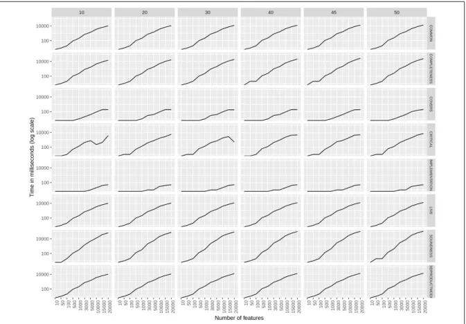
the Covers definition. Suppose the scopeF consisted of only two specifications{f1}and{f2}. Let’s
296
say that the two variants ( f1and f2) are mutually exclusive features. The implementation C= {c1, c2}
297
implements the feature f1, assumingT (f1) = {{c1}}andT (f2) = {{c2}}. Without the provision,
298
we would have Covers(C,{f1}). However, since Provided_by(C) = {f1, f2}, it actually implements
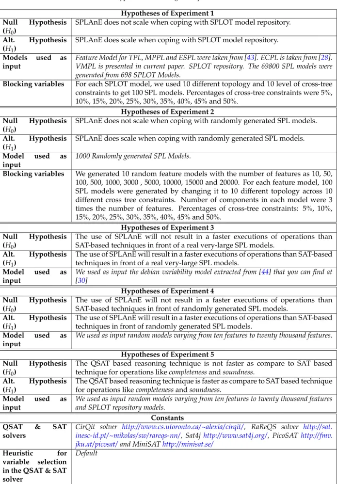
299
both the features together, thus violating the requirement of mutual exclusion. In the VMPL, the
300
implementation C6covers the specifications F1, F2, F3and F4. The set of products of the SPL is now
301
defined as the specifications and the implementations covering them through the traceability relation.
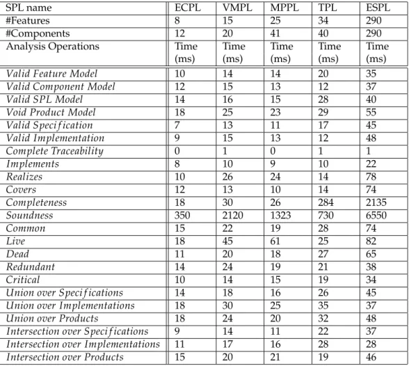
302
Definition 4(SPL Products). Given an SPLΨ= hF,C,T i, the products of the SPL, denoted by a function
303
Prod(Ψ)which generate a set of all specification-implementation pairshF, Ciwhere Covers(C, F).
304
Thus, in the VMPL example, we see that there are many potential products. Valid products are
305
hC1, F1i,hC2, F1i,hC3, F1i,hC3, F2i,hC4, F1i,hC4, F3i. . . .
306
4. Analysis Operations
307
Given an SPLΨ = hF,C,T i, we define the following analysis problems. The problems center
308
around the new definition of an SPL product.
SPL Model Verification:
310
Q. Is it a valid SPL model ? Is it a void SPL model ? Is the SPL model complete ?
311 312
A given SPL modelΨ = hF,C,T i is valid, if there exists a specification and implementation.
313
Let’s assume a feature model with three features f1, f2 and f3. The feature f1 is the root and the
314
features f2and f3 are the mandatory children of f1. An excludes relation exists between f2and f3.
315
The feature model cannot have any specification because of excludes relation and such SPL model is
316
not a valid model. A SPL models should be validated before analyzing any operations over it. Large
317
and complex SPLs undergoes continuous modification, such SPLs has to be verified for its validity
318
after every modification. In case of VMPLs, after adding new features, components and cross-tree
319
constraints, a validity of model should be tested. Is the virtual machine feature model and component
320
model valid?, such questions must be verified before further analysis of VMPL.
321
If all the features have a traceability relation with the components which implement them, such
322
a traceability relation is called as complete traceability relation. If there exists a feature which does
323
not have a traceability relation with any components, then such a traceability relation is called an
324
incomplete traceability relation. When a SPLs are under development, all the features many not
325
have its corresponding components developed. The operation complete traceability relation help us
326
to identify such features and proceed for its components development. The preliminary properties
327
valid model and complete traceability relation should hold before analyzing any other properties. Let
328
us assume an SPL modelhF,C,T iwhich is a valid model but none of the implementations Ci cover
329
any of the specification Fj. Such a model is called void product model i.e. the model is not able to
330
return a single product. In SPL model, it may happen that a feature model is valid, a component
331
model is valid and a traceability is also complete, but the SPL model is not able to generate a single
332
product. This is possible if no specification covers any of the implementation. A question like, Do
333
a Virtual Machine Product Line can generate at least one virtual machine ? is very important to conduct
334
further analysis of a product line.
335
Complete and Sound SPL:
336
Q. Does the SPL model is adequate for all the user specifications ? Do all implementation has it
337
corresponding specification ? Which are the useful implementations ? Is there at least one implementation
338
which realizes a given user specification ?
339 340
The completeness property of the SPL relates to the implementability of a specification. A
341
specification F is implementable if there is an implementation C such that Covers(C, F). Completeness
342
determines if the PL implementation (set of implementation variants) is adequate to provide
343
implementations for all the variant specifications in the PL specification. An SPLhF,C,T iis complete
344
if for every F∈ F, there is an implementation C∈ Csuch that Covers(C, F). The soundness property
345
relates to the usefulness of an implementation in an SPL. An implementation is said to be useful if it
346
implements some specification in the scope. An SPLhF,C,T iis sound if for every C ∈ C, there is a
347
specification F ∈ F such that Covers(C, F). The complete and sound are very crucial properties of
348
any SPLs. Does a VMPL is able to provide a virtual machine for every valid requirements (specifications) from
349
users?, if YES then the VMPL is complete. If there is some specification which cannot be implemented by
350
any of the implementation in the PL implementation, then such PL implementation is not adequate
351
to fill the wish of all the user specifications. In VMPL, there may be such requirements for which no
352
virtual machine can be generated. In such case, either feature model, component model or traceability
353
relation should be analyzed to figure out the actual problem. On the other hand, PL implementation
354
may provide huge set of implementation where as PL specification may be answered by a subset of
355
PL implementation. In case of VMPL, we may end up with such virtual machine which may not get
356
covered by any of the user specifications. Such machine should be removed from the pre-configured
357
machine list.
Product Optimization:
359
Q. Do the given specification and implementation, forms a product ? Is there an implementation which
360
provide all the features in a given user specification ? Is there an implementation exactly meeting a given user
361
specification ? Is there only one implementation for a given specification ?
362 363
Given a specification, we want to find out all the variant implementations that cover the
364
specification. This is given by a function FindCovers(F) = {C| Covers(C, F) }. At times, it is
365
necessary for a premier set of features to be provided exactly for some product variants. For example,
366
a client company with a critical usage of the product would limit the risk of feature interaction.
367
In this case, we want to find out if there is an implementation that realizes the specification. A
368
specification is existentially explicit if there exists an implementation C such that Realizes(C, F). Dually,
369
it is universally explicit if for all implementations C∈ C, Covers(C, F)implies Realizes(C, F). Multiple
370
implementations may implement a given specification. This may be a desirable criterion of the PL
371
implementation from the perspective of optimization among various choices. Thus, the specifications
372
which are implemented by only a single implementation are to be identified. F ∈ F has a unique
373
implementation if|FindCovers(F)| =1.
374
Is there a virtual machine which provide all the features as per the client specification? A covers is more
375
relaxed version where a specification is implemented by an implementation, but the implementation may
376
contain extra components which may not require to implement any of the features in a specification.
377
It may happen that, the cloud may have such pre-configured virtual machines which provides all the
378
features as per user specifications. Also this pre-configured machines has extra components which
379
are not required to support any of the features in user specifications. This may results in redundancy
380
of components in a virtual machine. Is there a virtual machine which provide exactly all the features as
381
per the client specification? The tighter version of cover is realize, which strictly does not allow any
382
extra components which are not required for features implementation present in a specification. A
383
realize is the optimized version of cover operation. Finding the optimized virtual machine on cloud
384
which match the exact user specifications is achieved by realize. Is there atleast one virtual machine
385
which provides exactly all the features as per the client specification? The existentially explicit operations
386
guarantee the presence of at least one implementation which is realized by a given specifications.
387
It means, in VMPL for a user specification there exists at least one virtual machine which realizes
388
it and this guarantees the presence of at least one optimized configuration. The universally explicit
389
is the tighter version of existentially explicit, which means all the implementation covers by a given
390
specification implies that it is an realization. For universally explicit specifications, cloud always
391
produce the optimized virtual machine. Does a given user specification has only one virtual machine
392
provided by cloud? In VMPL, there may be some specification which is covered by only one virtual
393
machine, such implementations are unique.
394
SPL Optimization:
395
Q. Does an element is present across all the products ? Does an element is used in at least single product
396
? Does an element not in use ? Which all elements are redundant in a given product ? Which are the extra
397
features provided by a product apart from the given user specification ?
398 399
Identification of common, live and dead elements in an SPL are some of the basic analyses
400
operations in the SPL community. We redefine these concepts in terms of our notion of products:
401
An element e is common if for allhF, Ci ∈ Prod(Ψ), e ∈ F∪C. An element e is live if there exists
402
hF, Ci ∈ Prod(Ψ)such that e ∈ F∪C. An element e is dead if for allhF, Ci ∈ Prod(Ψ), e 6∈ F∪C.
403
Now a days with the advance in technology, business changes it requirements so quickly that, exiting
404
products in market get replaced by another advance products in a very short time span. As the SPLs
405
evolves, new cross-tree constraints get added or removed, this results in change of products. Due to
406
such modification, few features or components in SPL may become live or dead. Do the component c is
present in at least one virtual machine provided by VMPL? Do the component c is not present in any of the
408
virtual machines provided by VMPL? The common property find all the common elements (features or
409
components) across all the products. This operation is required to create a common platform for a
410
SPL. Do the component c is present in all the virtual machines provided by VMPL?
411
There may be certain implementations that are useful but the implementable specifications
412
are not affected if these implementations are dropped from the PL implementation. These
413
implementations are called superfluous. Formally, an implementation C ∈ Cis superfluous if for all
414
F ∈ F such that Covers(C, F), there is a different implementation D ∈ C such that Covers(D, F).
415
Superfluousness is relative to a given PL implementation. If in an SPL Ψ, F = {{f}}, C = 416
{{a},{b}} and T (f) = {{a},{b}}, then both the implementations {a} and {b} are superfluous
417
w.r.t. Ψ, whereas if either {a} or {b} is removed from the PL implementation, the remaining
418
implementation ({b}or{a}) is not superfluous anymore (w.r.t. the reduced SPL). The feature Java
419
in VMPL, can be implemented by component OpenJDK or OracleJDK. Such traceability results in
420
many superfluous implementations . Superfluousness for a specification guarantees the presence
421
of alternate implementations.
422
Which are the components in the virtual machines that can be removed without impacting the user
423
specification ? A component is redundant if it does not contribute to any feature in any implementation
424
in the SPL. A component c ∈ C is redundant if for every C ∈ C, we have Provided_by(C) = 425
Provided_by(C\ {c})). An SPL can be optimized by removing the redundant components without
426
affecting the set of products. Redundant elements may not be dead. Due to the packaging, redundant
427
elements can be part of useful implementations of the SPL and hence be live. Do the component c is
428
required for any of the features in a user specification? A component c is critical for a feature f in the SPL
429
scopeF, when the component must be present in an implementation that implements the feature f :
430
for all implementations C∈ C,(c 6∈C =⇒ ¬implements(C, f)). This definition can be extended to
431
specifications as well: a component c is critical for a specification F, if for all implementations C∈ C,
432
(c6∈C =⇒ ¬Covers(C, F)). A virtual machine may contain components which may not be required
433
for any of the features in a user specifications, but it may remain due to packaging. Such components
434
are redundant but not critical.
435
Can virtual machine provide more features with the same set of components? When a specification
436
is covered (but not realized) by an implementation, there may be extra features (other than those
437
in the specification) provided by the implementation. These extra features are called extraneous
438
features of the implementation. Since there can be multiple covering implementations for the
439
same specification, we get different choices of implementation and extraneous features pairs :
440
Extra(F) ≡ {hC, Provided_by(C) \Fi|Covers(C, F)}. User may demand for virtual machines
441
with some specification. The available pre-configured machine provide all the features in user
442
specification, and also provide few more features which are extraneous.
443
Generalization and Specialization in SPL:
444
Do the union of two or more products result in a new product ? What is the difference between two
445
products ?
446 447
In an SPL, sometimes there is a need to check the aggregation relationship between the
448
specifications, implementations or products. Is there a virtual machine which has features provided by a
449
given set of virtual machines? The union property on two specifications will result in a new specification
450
which has features of both the specifications. Let’s say specification F1 has features{f1, f2, f3}and
451
specification F2 has features {f2, f5, f7}. The union property will check for some specification F
452
which has features of specifications F1and F2, so F should have features{f1, f2, f3, f5, f7}. Assume an
453
excludes relation between features f3and f5, then the union property will return FALSE. In VMPL, the
454
user always demand a virtual machines which has equivalent features of two or more machines. The
union property is used to verify the combination of two or more virtual machines is valid. Similar to
456
specifications, this property can be applied on implementations or products.
457
In an SPL, most of the time there is a need to distinguish between the multiple specifications or
458
implementations or products. Is there a virtual machine those features are present in all virtual machines
459
in a given set? The intersection property on multiple specifications will check the existence of any
460
specification which is common to those specifications. Let’s say specification F1 = {f1, f2, f3} and
461
F2 = {f1, f2, f7}, then the intersection property applied on specification F1 and F2 will result in
462
specification F = {f1, f2}. The distinguishable features or variants between F1and F2are obtained
463
as F1\F = {f3}and F2\F = {f7}. A specification which is contained in all the specifications of an
464
SPL is called core speci f ication. The intersection property applied on a given SPL model will result
465
in a core speci f ication. Similar to specifications, this property can be applied to implementations or
466
products.
467
In the literature, different analysis problems in SPLs are usually encoded as satisfiability
468
problems for propositional constraints [33] and SAT solvers such as Yices [34] or Bddsolve [35] are
469
used to solve them. As it has been noted in [20], it is not possible to cast certain problems such as
470
completeness and soundness as a single propositional constraint. However, we observe that these
471
problems need quantification over propositional variables encoding features and components. The
472
most expressive logic formalism, Quantified Boolean Formula (QBF), is necessary to encode such
473
analysis problems. The Boolean satisfiability problem for a propositional formula is then naturally
474
extended to a QBF satisfiability problem (QSAT).
475
The tool SPLAnE provide analysis operations - valid model, complete traceability, void product
476
model, implements, covers, realizes, soundness, completeness, existentially explicit, universally
477
explicit, unique implementation, common, live, dead superfluous, redundant, critical, union and
478
intersection. SPLAnE encode each analysis operation in single QBF. The tool FaMa provide analysis
479
operations - commonality, core features, dead feature, detect error, explain error, filter question,
480
unique feature, variability question, valid configuration, variant feature and valid product[6]. FaMa
481
encode each analysis operation in single propositional formula. Every analysis operation of FaMa
482
can be encoded in QBF and can be solved by SPLAnE , where as the formula like soundness cannot
483
be encoded in a single SAT formula. To compare our QSAT approach with SAT approach we
484
implemented analysis operation provided by SPLAnE on FaMa. There are few analysis operations
485
provided by SPLAnE like valid model, complete traceability, void product model, implements,
486
covers, realizes and live which uses only one existential quantifiers or universal quantifier, and can be
487
encoded in SAT and executed with FaMa. The operations like soundness, completeness, existentially
488
explicit and universally explicit cannot be encoded in single SAT, so for experimental comparison
489
such formula is executed with FaMa in iteration.
490
In SPLs, the complexity of analysis operations, like valid model or void product model which can
491
be represented using propositional logic belongs to∑1P = ∃P(Φ), where p is the class of all feasibly
492
decidable languages [36]. We found few analysis operations discussed in this paper like soundness or
493
completeness that cannot be encoded using SAT formulae, but easily by using QBFs. The complexity of
494
the soundness and completeness operations belongs to the classΠ2P= ∀P∑P1. More complex analysis
495
operations, like universally explicit, unique implementation belongs to the class ∑P3 = ∃PΠP2 [36].
496
Similarly, QBF can be easily used to represent formula belonging to more complex classes.
497
LetC = {c1, . . . , cn}be the core assets and letF = {f1, . . . , fm}be the scope of the SPL. Each
498
feature and component x is encoded as a propositional variable px. Given an implementation C, bC
499
denotes the formula V
ci∈Cpci, and ¯C denotes a bitvector where ¯C[i] = 1 (TRUE) if ci ∈ C and 0 500
(FALSE) otherwise. Similarly, for a specification F, we have bF and ¯F.
501
Let CONF and CONI denote the set of constraints over the propositional variables capturing
502
the PL specification and PL implementation respectively. Given the PL specification and PL
503
implementations as sets, it is straightforward to get these constraints. When one uses richer notations,
504
like feature models, one can extract these constraints following [33]. For the traceability, the encoding
CONTis as follows. Let f be a feature and letT (f) = {C1, C2. . . , Ck}. We define f ormula_T (f)as
506 W
j=1..kVci∈Cjpci. If the setT (f)is undefined(empty), then f ormula_T (f)is set to FALSE. CONTis 507
then defined asV
fi∈F [f ormula_T (fi) =⇒ pfi] for the features fi for whichT (fi)is defined and 508
FALSE ifT (.)is not defined for any feature.
509
The implementation question whether implements(C, f)is now answered by asking whether
510
the formula bC for the set of components C along with the traceability constraints CONT can
511
derive the feature f . This is equivalent to asking whether bC∧CONT∧ (¬pf) is UNSAT. Since
512
it is evident that onlyT (f) is used for the implementation of f , this can further be optimized to
513
b
C∧ (f ormula_T (f) ⇒ pf) ∧ (¬pf). However, as we will see later, since implements(., .)is used as
514
an auxiliary function in the other analyses, we want to encode it as a formula with free variables.
515
Thus, f orm_implementsf(x1, . . . , xn)is a formula which takes n Boolean values (0 or 1) as arguments,
516
corresponding to the bitvector ¯C of an implementation C and evaluates to either TRUE or FALSE.
517 518 f orm_implementsf(x1, . . . , xn) = ∀pc1. . . pcn{[ Vn i=1(xi⇒pci)] ⇒ f ormula_T (f)}. 519 520
This forms the core of encoding for all the other analyses. Hence, the correctness of this
521
construction is crucial. Lemma1states the correctness result. The proof is given in [37].
522
Lemma 1. (Implements) Given an SPL, a set of components C, and a feature f ,implements(C, f)iff
523
f orm_implementsf(v1, . . . , vn), where ¯C= hv1, . . . , vni, evaluates to TRUE.
524
In order to extend the construction to encode Covers, we construct a formula f _covers(x1, . . . ,
525
xn, y1, . . . , ym)where, the first n Boolean values encode an implementation C and the subsequent m
526
Boolean values encode a specification F. The formula evaluates to TRUE iff Covers(C, F)holds.
527 528
f _covers(x1, . . . , xn, y1, . . . , ym)=Vi=1m [yi ⇒ f orm_implementsfi(x1, . . . , xn)]. 529
530
Similarly, we have encoded Realizes in a Quantified Boolean Formula as below. Notice the
531
replacement of “⇒” in f _covers(..)by “⇔” in f _realizes(..).
532 533
f _realizes(x1, . . . , xn, y1, . . . , ym)=Vi=1m [yi ⇔ f orm_implementsfi (x1, . . . , xn)]. 534
535
In VMPL, we ask whether Covers(C2, F1). Since there are 20 components {c1. . . c20} and 15
536
features{f1. . . f15}, this translates to the formula f _covers(1, 1, 1, 0, 1, 0, 0, 0, 0, 0, 0, 0, 0, 0, 0, 0, 0, 0,
537
0, 0, 1, 1, 1, 0, 0, 0, 0, 0, 0, 0, 0, 0, 0, 0, 0). For each feature in the specification F1, simplification boils
538
down to f orm_implementsf1(1, 1, 1, 0, 1, 0, 0, 0, 0, 0, 0, 0, 0, 0, 0, 0, 0, 0, 0, 0), similarly for f2to f15. 539
Since f ormula_T (f1) =pc1, after simplification we get∀pc1. . . pc20 {(1 ⇒ pc1 ∧1 ⇒ pc2 ∧1 ⇒ pc3 540
∧0 ⇒ pc4 ∧1⇒ pc5 ∧0 ⇒ pc6 ∧0 ⇒ pc7 ∧0⇒ pc8 ∧0 ⇒ pc9 ∧0 ⇒ pc10 ∧0 ⇒ pc11 ∧0 ⇒ pc12
541
∧ 0 ⇒ pc13 ∧ 0 ⇒ pc14 ∧ 0 ⇒ pc15 ∧ 0 ⇒ pc16 ∧ 0 ⇒ pc17 ∧0 ⇒ pc18 ∧0 ⇒ pc19 ∧0 ⇒ pc20 )
542
⇒ (pc1)}. The formula f orm_implementsf1 holds true, so we check the formula f orm_implementsfi 543
for remaining features in the specification F1. Since it is true for all the features, the Covers(C2, F1)
544
holds.
545
In order to demonstrate a negative example, we ask whether Covers(C2, F2). We simplify the
546
encoded formula f _covers(1, 1, 1, 0, 1, 0, 0, 0, 0, 0, 0, 0, 0, 0, 0, 0, 0, 0, 0, 0, 1, 1, 1, 1, 1, 0, 0, 0, 0, 0, 0, 0, 0,
547
0, 0), with f ormula_T (f4) = pc6. This yields f orm_implementsf4(1, 1, 1, 0, 1, 0, 0, 0, 0, 0, 0, 0, 0, 0, 0, 548
0, 0, 0, 0, 0)and at last,∀pc1. . . pc20{(1⇒pc1 ∧1⇒pc2 ∧1⇒pc3 ∧0⇒pc4 ∧1⇒pc5 ∧0⇒pc6 ∧ 549
0⇒ pc7 ∧0⇒ pc8 ∧0⇒ pc9 ∧0 ⇒pc10∧0⇒ pc11 ∧0⇒pc12 ∧0 ⇒pc13∧0⇒ pc14 ∧0 ⇒pc15 ∧ 550
0⇒ pc16 ∧0⇒ pc17 ∧0 ⇒pc18 ∧0 ⇒pc19∧0⇒ pc20) ⇒ (pc6)}. Since this is FALSE, we conclude
551
correctly that Covers(C2, F2)does not hold.
552
We encode the other analysis problems as QBF formulae as shown in Table2. The theorem 5 553
asserts the correctness of the encoding. In the theorem, for the constraint CONI, CONI[qc1, . . . , qcn] 554
denotes the same constraint where each propositional variable pci has been replaced by a new 555
propositional variable qci. 556
Theorem 5. Given an SPLΨ, each of the properties listed in Table2holds if and only if the corresponding
557
formula evaluates to true.
558
Proof. The proof can be seen in [37].
559
Table 2.Properties and Formulae
Properties Formula
Valid Model ∃pf1. . . pfm∃pc1. . . pcn[CONI] ∧ [CONF]
Complete Traceability ∃pc1. . . pcn{(T (pf1) ∧ · · · ∧ T (pfm)) =⇒ (pc1∨pc2∨ · · · ∨pcn)}
Void Product Model ∃pf1. . . pfm∃pc1 . . . pcn[CONI] ∧ [CONF] ∧ ¬f _covers(pc1, . . . , pcn,
pf1, . . . , pfm) Implements(C, f) f orm_implementsf(v1, . . . , vn) ¯ C= (v1, . . . , vn) Covers(C, F) f _covers(v1, . . . , vn, u1, . . . , um) Realizes(C, F) f _realizes(v1, . . . , vn, u1, . . . , um) ¯ C= (v1, . . . , vn), ¯ F= (u1, . . . , um) Ψ complete ∀pf1. . . pfm{CONF⇒ ∃pc1. . . pcn[CONI∧ f _covers(pc1, . . . , pcn, pf1, . . . , pfm)]}
Ψ sound ∀pc1. . . pcn {CONI ⇒∃pf1 . . . pfm [CONF ∧ f _covers(pc1, . . . , pcn,
pf1, . . . , pfm)]}
F existentially explicit ∃pc1. . . pcn{CONI∧f _realizes(pc1, . . . , pcn, u1, . . . , um)}
¯
F= (u1, . . . , um)
F universally explicit ∃pc1. . . pcn{CONI∧f _realizes(pc1, . . . , pcn, u1, . . . , um)} ∧
¯
F= (u1, . . . , um) ∀pc1. . . pcn {[(CONI∧ f _covers(pc1, . . . , pcn, u1, . . . , um)] ⇒
f _realizes(pc1, . . . , pcn, u1, . . . , um)}.
F has unique implementation ∃pc1. . . pcn[CONI∧ f _covers(pc1, . . . , pcn, u1, . . . , um)]∧
¯
F= (u1, . . . , um) ∀qc1 . . . qcn((CONI[qc1 . . . qcn] ∧ f _covers(qc1, . . . , qcn, u1, . . . , um))
⇒ (∧n
l=1(pcl ⇔qcl)))]
cicommon ∀pc1. . . pcnpf1 . . . pfm{(CONI∧CONF∧
f _covers(pc1, . . . , pcn, pf1, . . . , pfm)) ⇒pci}
cilive ∃pc1. . . pcn, pf1. . . pfm{(CONI∧CONF∧
f _covers(pc1, . . . , pcn, pf1, . . . , pfm)) ∧pci}
c dead ∀pc1 . . . pcnpf1 . . . pfm{(CONI ∧CONF∧
f _covers(pc1, . . . , pcn, pf1, . . . , pfm)) ⇒ ¬pci}
C superfluous ∀pf1. . . pfm[(CONF∧ f _covers(v1, . . . , vn, pf1, . . . , pfm)) ⇒
¯
C= (v1, . . . , vn) ∃pc1. . . pcn(CONI∧ ∨i=1..n(pci 6=vi)∧
f _covers(pc1, . . . , pcn, pf1, . . . , pfm))]
ciredundant ∀pc1. . . pcnpf1. . . pfm{(pci∧CONI∧CONF∧
f _covers(pc1, . . . , pcn, pf1, . . . , pfm)) ⇒
f _covers(pc1, . . . ,¬pci, . . . , pcn, pf1, . . . , pfm)}
cicritical for fj ∀pc1. . . pcn[f orm_implementsfj(pc1. . . pcn) ⇒ pcj]
Union ∃pf11, . . . , pf1n ∃pf21, . . . , pf2n ∃f1, . . . fn {f1⇔ (pf11 ∨pf21) . . .
fn⇔ (pf1n∨pf2n) ∧ [CONF]}
Intersection ∃pf11, . . . , pf1n ∃pf21, . . . , pf2n∃f1, . . . fn {f1⇔ (pf11 ∧pf21) . . . fn
5. Validation
560
In order to validate the approach presented in this paper, a tool SPLAnE for the automated
561
analysis of SPL models has been developed. SPL models consists of feature models with traceability
562
relationships to the component models (Core assests). The Virtual Machine Product Line (VMPL)
563
case study based on cloud computing concepts is presented and analyzed.
564
5.1. SPLAnE
565
SPLAnE (Software Product Line Analysis Engine) is designed and developed to analyze the
566
traceability between the features and implementation assets. Nowadays, there is the large set of tools
567
that enable the reasoning over feature models. However, none of them is capable of reasoning over
568
the feature model and a set of implementations as described throughout this paper. For the sake
569
of reusability and because it has been proven to be easily extensible [38,39], we chose to use the
570
FaMa framework [29] as the base for SPLAnE . The FaMa framework provides a basic architecture for
571
building FM analysis tools while defining interfaces and standard implementation for existing FM
572
operations in the literature such as Valid Model or Void Product Model.
573
On the one hand, SPLAnE benefits from being a FaMa extension in different ways. For example,
574
SPLAnE can read a large set of different file formats used to describe feature models. It is also possible
575
to perform some of the existing operations in the literature to the feature model prior to executing
576
the reasoning over the component layer. On the other hand, FaMa was not designed for reasoning
577
over more than one model. Therefore, different modifications have been addressed to fill this gap.
578
Namely, i) we modified the architecture to enable this new extension point into the FaMa architecture;
579
ii) created a new reasoner for a new set of operations; iii) implemented the operations, and iv) defined
580
two new file formats to store and input traceability relationships and component models in SPLAnE .
581
Figure 4.SPLAnE reasoning process
The reasoning process performed by SPLAnE is shown in the Figure 4. First, SPLAnE takes
582
as input a feature model, a traceability relationship and a component model. The SPLAnE parser
583
creates the SPL model from this input files. Second, SPLAnE constructs the QBF/QCIR formula
584
based on the selected analysis operations. QBF is further encoded in QPRO format, this is done by
585
SPLAnE translator. QPRO [40] and QCIR [41] format is a standard input file format in non-prenex,
586
non-CNF form. Later, SPLAnE invokes the QSAT solver CirQit [26] or RaReQS [27] in the back-end to
587
check the satisfiability of the generated QBFs in QPRO/QCIR format. The choice of the tool is based
588
upon its performance: CirQit has solved the most number of problems in the non-prenex, non-CNF
track of QBFEval’10 [42]. RaReQS [27] is a Recursive Abstraction Refinement QBF Solver. Table2 590
shows the analysis operations provided by SPLAnE .
591
The design of SPLAnE makes it possible to use different QSAT solvers. Also, SPLAnE can now
592
work hand in hand with other products based on FaMa such as Betty [29], which enables the testing
593
of feature models. SPLAnE is now available for download with its detailed documentation from the
594
website [30].
595
5.2. Experimentation
596
In this section, we go through the different experiments executed to validate our approach.
597
The experiments was conducted with i) Real debian models, ii) Randomly generated models and
598
iii) SPLOT Repository models. Each analysis operation was executed with two QSAT solver (CirQit
599
and RaReQS) and three SAT solver (Sat4j, PicoSAT and MiniSAT). All experiments was run on a 3.2
600
GHz i7 processor machine with 16 GB RAM. The experimentation results are plotted in graph with
601
log scale. Also on the graph plot, solver names are denoted as {qcir: CirQit, qrare: RaReQS, psat:
602
PicoSAT, msat: MiniSAT}. Table3shows the hypothesis and the variables used when conducting this
603
experimentation.
604
5.2.1. Experiment 1: Validating SPLAnE with feature models from the SPLOT repository
605
To illustrate the SPL analysis method described in the paper, we considered case studies of
606
various sizes. Concretely, the following SPLs were used: Entry Control Product Line (ECPL), Virtual
607
Machine Product Line (VMPL), Mobile Phone Product Line (MPPL), Tablet Product Line (TPL) and
608
Electronic Shopping Product Line (ESPL). The TPL, MPPL, and ESPL models were taken from the
609
SPLOT repository [43]. More details of the ECPL models can be found at [28]. Table4 gives the
610
number of features, components in each SPL model, and the execution time taken by various analysis
611
operations on SPLAnE reasoner - CirQit.
612 613
The SPLOT repository is a common place where a practitioners store feature models for the
614
sake of reuse and communication. The SPLOT repository contains small and medium size feature
615
models, most of it are conceptual and few are realistic. We extracted 698 feature models from the
616
SPLOT repository. These feature models were given as an input to extended Betty tool to generate
617
corresponding SPL models. Usually, components models which represent the solution space of
618
SPLs are larger in size. So, the generated component models contain 3 times more components
619
then the number of features present in the corresponding feature model. SPLAnE generated the
620
random traceability relation between feature model and component model to generate a complete
621
SPL model. Further, to increase the complexity of experiments, each SPL model is generated
622
using 10 different topologies and 10 different level of cross-tree constraints with percentage as
623
{5, 10, 15, 20, 25, 30, 35, 40, 45, 50}, resulting in a total of 100 SPL models per SPLOT model. So from
624
698 SPLOT models, we got 69800 SPL models. The percentage of cross-tree constraint is defined by
625
the percentage of constraints over the number of features. Basically it is the number of constraints
626
depending on the number of features. For example, if we specify a 50% percentage over a model with
627
10 features, then we have 5 cross-tree constraints.
628
The tool SPLAnE was executed with 69800 SPL models to verify the QSAT scalability when
629
applying it to feature modeling. SPLAnE provide an option to select any one of the two QSAT
630
reasoners (CirQit and RaReQS). Figure5shows the box plot, representing the QSAT behaviour with
631
increase in cross-tree constraints for few analysis operations on real models taken from the SPLOT
632
repository. This experiment was executed with the QSAT reasoner CirQit. The results for experiment
633
5.2.1shows that for the small and medium size real models, all analysis operations does not take
634
much execution time which motivated us to experiments with large size models. The overall results
635
for experiment5.2.1point out that the null hypothesis H0was wrong, thus, resulting in the acceptance
636
of the alternative hypothesis H1.
Table 3.Hypotheses and design of experiments.
Hypotheses of Experiment 1 Null Hypothesis
(H0)
SPLAnE does not scale when coping with SPLOT model repository. Alt. Hypothesis
(H1)
SPLAnE does scale when coping with SPLOT model repository. Models used as
input
Feature Model for TPL, MPPL and ESPL were taken from [43]. ECPL is taken from [28]. VMPL is presented in current paper. SPLOT repository. The 69800 SPL models were generated from 698 SPLOT Models.
Blocking variables For each SPLOT model, we used 10 different topology and 10 level of cross-tree constraints to get 100 SPL models. Percentages of cross-tree constraints were 5%, 10%, 15%, 20%, 25%, 30%, 35%, 40%, 45% and 50%.
Hypotheses of Experiment 2 Null Hypothesis
(H0)
SPLAnE does not scale when coping with randomly generated SPL models. Alt. Hypothesis
(H1)
SPLAnE does scale when coping with randomly generated SPL models. Model used as
input
1000 Randomly generated SPL Models.
Blocking variables We generated 10 random feature models with the number of features as 10, 50, 100, 500, 1000, 3000 , 5000, 10000, 15000 and 20000. For each feature model, 100 SPL models were generated by changing it to 10 different topology across 10 different cross tree constraints. Number of components in each model were 3 times the number of features. Percentages of cross-tree constraints: 5%, 10%, 15%, 20%, 25%, 30%, 35%, 40%, 45% and 50%.
Hypotheses of Experiment 3 Null Hypothesis
(H0)
The use of SPLAnE will not result in a faster executions of operations than SAT-based techniques in front of a real very-large SPL models.
Alt. Hypothesis (H1)
The use of SPLAnE will result in a faster executions of operations than SAT-based techniques in front of a real very-large SPL models.
Model used as input
We used as input the debian variability model extracted from [44] that you can find at [30]
Hypotheses of Experiment 4 Null Hypothesis
(H0)
The use of SPLAnE will not result in a faster executions of operations than SAT-based techniques in front of randomly generated SPL models.
Alt. Hypothesis (H1)
The use of SPLAnE will result in a faster executions of operations than SAT-based techniques in front of randomly generated SPL models.
Model used as input
We used as input random models varying from ten features to twenty thousand features. Hypotheses of Experiment 5
Null Hypothesis (H0)
The QSAT based reasoning technique is not faster as compare to SAT based technique for operations like completeness and soundness.
Alt. Hypothesis (H1)
The QSAT based reasoning technique is faster as compare to SAT based technique for operations like completeness and soundness.
Model used as input
We used as input random models varying from ten features to twenty thousand features and SPLOT repository models.
Constants QSAT & SAT
solvers
CirQit solver http://www.cs.utoronto.ca/~alexia/cirqit/, RaReQS solver http://sat.
inesc-id.pt/~mikolas/sw/rareqs-nn/, Sat4j http://www.sat4j.org/, PicoSAT http://fmv.
jku.at/picosat/ and MiniSAThttp://minisat.se/
Heuristic for variable selection in the QSAT & SAT solver
COMMON COMPLETENESS CO VERS CRITICAL IMPLEMENTS LIVE NO TCRITICAL SOUNDNESS V ALIDMODEL V OIDPR ODUCTMODEL 0 500 1000 1500 2000 2500 3000 3500 4000 0 500 1000 1500 2000 2500 3000 3500 4000 REAL−FM−1.xml REAL−FM−10.xml REAL−FM−11.xml REAL−FM−12.xml REAL−FM−13.xml REAL−FM−14.xml REAL−FM−15.xml REAL−FM−16.xml REAL−FM−17.xml REAL−FM−18.xml REAL−FM−19.xml REAL−FM−2.xml REAL−FM−20.xml REAL−FM−3.xml REAL−FM−4.xml REAL−FM−5.xml REAL−FM−6.xml REAL−FM−7.xml REAL−FM−8.xml REAL−FM−9.xml REAL−FM−1.xml REAL−FM−10.xml REAL−FM−11.xml REAL−FM−12.xml REAL−FM−13.xml REAL−FM−14.xml REAL−FM−15.xml REAL−FM−16.xml REAL−FM−17.xml REAL−FM−18.xml REAL−FM−19.xml REAL−FM−2.xml REAL−FM−20.xml REAL−FM−3.xml REAL−FM−4.xml REAL−FM−5.xml REAL−FM−6.xml REAL−FM−7.xml REAL−FM−8.xml REAL−FM−9.xml REAL−FM−1.xml REAL−FM−10.xml REAL−FM−11.xml REAL−FM−12.xml REAL−FM−13.xml REAL−FM−14.xml REAL−FM−15.xml REAL−FM−16.xml REAL−FM−17.xml REAL−FM−18.xml REAL−FM−19.xml REAL−FM−2.xml REAL−FM−20.xml REAL−FM−3.xml REAL−FM−4.xml REAL−FM−5.xml REAL−FM−6.xml REAL−FM−7.xml REAL−FM−8.xml REAL−FM−9.xml REAL−FM−1.xml REAL−FM−10.xml REAL−FM−11.xml REAL−FM−12.xml REAL−FM−13.xml REAL−FM−14.xml REAL−FM−15.xml REAL−FM−16.xml REAL−FM−17.xml REAL−FM−18.xml REAL−FM−19.xml REAL−FM−2.xml REAL−FM−20.xml REAL−FM−3.xml REAL−FM−4.xml REAL−FM−5.xml REAL−FM−6.xml REAL−FM−7.xml REAL−FM−8.xml REAL−FM−9.xml REAL−FM−1.xml REAL−FM−10.xml REAL−FM−11.xml REAL−FM−12.xml REAL−FM−13.xml REAL−FM−14.xml REAL−FM−15.xml REAL−FM−16.xml REAL−FM−17.xml REAL−FM−18.xml REAL−FM−19.xml REAL−FM−2.xml REAL−FM−20.xml REAL−FM−3.xml REAL−FM−4.xml REAL−FM−5.xml REAL−FM−6.xml REAL−FM−7.xml REAL−FM−8.xml REAL−FM−9.xml Input model Time in milliseconds Figure 5. Impact on QSA T scalability on Real SPLOT models with the incr ement in CTC levels.