On the irregular behavior of LS estimators for asymptotically singular designs

HAL Id: hal-00416062

https://hal.archives-ouvertes.fr/hal-00416062

HAL is a multi-disciplinary open access

archive for the deposit and dissemination of sci-entific research documents, whether they are pub-lished or not. The documents may come from

L’archive ouverte pluridisciplinaire HAL, est destinée au dépôt et à la diffusion de documents scientifiques de niveau recherche, publiés ou non, émanant des établissements d’enseignement et de

On the irregular behavior of LS estimators for

asymptotically singular designs

Andrej Pazman, Luc Pronzato

To cite this version:

Andrej Pazman, Luc Pronzato. On the irregular behavior of LS estimators for asymptot-ically singular designs. Statistics and Probability Letters, Elsevier, 2006, 76, pp.1089-1096. �10.1016/j.spl.2005.12.010�. �hal-00416062�

On the irregular behavior of LS estimators for

asymptotically singular designs ⋆

Andrej P´azman

and Luc Pronzato

∗

Mlynsk´a Dolina, 84248 Bratislava, Slovakia

b_{Laboratoire I3S, CNRS/UNSA, Bˆat. Euclide, Les Algorithmes,}

2000 route des Lucioles, BP 121, 06903 Sophia-Antipolis Cedex, France

Abstract

Optimum design theory sometimes yields singular designs. An example with a linear regression model often mentioned in the literature is used to illustrate the difficulties induced by such designs. The estimation of the model parameters θ, or of a function of interest h(θ), may be impossible with the singular design ξ∗. Depending on how ξ∗ is approached by the empirical measure ξn of the design points, with n the number

of observations, consistency is achieved but the speed of convergence may depend on ξn and on the value of θ. Even in situations where convergence is in 1/√n and

the asymptotic distribution of the estimator of θ or h(θ) is normal, the asymptotic variance may still differ from that obtained from ξ∗.

Key words: singular design, optimum design, asymptotic normality, consistency, LS estimation

PACS: 62K05, 62E20

⋆ The research of the 1st author has been supported by the VEGA-grant nb. 1/0264/03. The research of the 2nd author has been supported in part by the IST Programme of the European Community under the PASCAL network of Excellence IST2002506778. This publication only reflects the authors views.

∗ author for correspondence

Email addresses: pazman@fmph.uniba.sk (Andrej P´azman), pronzato@i3s.unice.fr (Luc Pronzato).

1 Introduction

We consider the following linear regression model

η(x, θ) = θ1x + θ2x2 = f⊤(x)θ (1)

with f (x) = (x, x2₎⊤_{, x ∈ X = [−1, 1] and observations y}

k = η(xk, ¯θ) + εk

where ¯θ is the (unknown) true value of the model parameters and the errors εk

are i.i.d. with zero mean and variance σ2_{. We shall take σ = 1 throughout the}

paper. We shall denote ˆθn_{the LS estimator of θ obtained from the observations}

y1, y2, . . . , yn; ξn will denote the empirical measure of the associated design

points x1, x2, . . . , xn. We shall also denote

M(ξ) =

Z

X

f(x)f⊤(x) ξ(dx)

the information matrix for a design measure ξ.

We assume that ¯θ1 ≥ 0 and ¯θ2 < 0 and are interested in the estimation of

h(θ) =− θ1

2θ2

, (2)

the value of x where η(x, θ) is maximal. When the design space isX = [−1, 1],

the optimum design measure ξ∗ _{= ξ}∗

θ for the estimation of h(θ) (c-optimality)

has its support included in{−1, 1}, the weight of each point depending on the

value of h(θ) (a standard situation in nonlinear problems). One can show, see, e.g., Silvey (1980, p. 57), that

ξ∗(1) =      1 2 + 1 4h if h≥ 1 2, 1 2 + h if 0≤ h ≤ 1 2, (3)

so that when h(θ) = 1/2 the optimum design is singular with ξ∗_{(1) = 1 (and}

ξ∗_{(−1) = 0). Therefore, if we know a priori that h(¯θ) is close to 1/2 we should}

put the design points, or the majority of them, close to 1. It is the purpose of this paper to show that depending how this is realized, the asymptotic

behavior of ˆθn_{, or of h(ˆθ}n_{), may have some unexpected features. Note that}

h(θ) is not estimable when ξ∗ _{is singular. Therefore, when h(ˆθ}n_{) obtained}

with the design ξn converges to h(¯θ), n → ∞, it means that the sequence

x1, x2, . . . itself, not the limiting design ξ∗, is responsible for consistency. In

particular, it thus seems legitimate to question the adjective “optimum” for ξ∗_.

The example considered is extremely simple but the conclusions are of general consequences: we show that it is only in very particular circumstances that approaching a singular “optimum” design conveys some optimal properties to the nonlinear LS estimation for which it was designed. The example has been chosen due to its frequent use in the optimum-design literature, see e.g. Silvey (1980); Ford and Silvey (1980); Ford et al. (1985); Wu (1985). Here, the

singularity of ξ∗ _{is obtained for a particular value of h(θ). This should not give}

the reader the impression that singular “optimum” designs are exceptional. For

instance, the estimation of h(θ) = _−θ1/(2θ2) in the full quadratic regression

model η(x, θ) = θ0 + θ1x + θ2x2 yields singular “optimum” designs for a full

range of values of h, see Chaloner (1989); Fedorov and M¨uller (1997). See also

Buonaccorsi and Iyer (1986) for the estimation of ratios of linear combinations of the parameters.

Sections 2 and 3 concern the situation where we know a priori that h(¯θ) is

close to 1/2 and non-sequential designs approaching the singular measure ξ∗

are used: ξn converges weakly to ξ∗ in Section 2 whereas strong convergence

is considered in Section 3. The iterative construction of the design is briefly discussed in Section 4. Throughout the paper we denote

1=    1 1    and 0 =    0 0    . 2 ξn converges weakly to ξ∗

By weak convergence we mean convergence in distribution, which we denote

w

→. Let ξ∗ _{be the singular measure that puts weight 1 at x = 1. Throughout}

the section we use the design measure ξn constructed from

xi =      1 if i = 2k− 1 , 1 + (1/k)1/4 _{if i = 2k ,} for k = 1, 2, . . . so that ξn → ξw ∗, n→ ∞.

2.1 Consistency.

From Corollary 1 of (Wu, 1980), u⊤_θˆn a.s._{→ u}⊤_{θ for any u}¯ _{∈ R}2 _{when S}∞_{(w) =}

P∞

i=1[w⊤f(xi)]2 =∞ for all w = (w1, w2)⊤6= 0. Here we obtain

S∞(w) = ∞ X k=1 (w1+ w2)2+ ∞ X k=1 n w1[1 + 1/k1/4] + w2[1 + 1/k1/4]2 o2 so that S∞_{(w) = ∞ when w}

1 + w2 6= 0. For w1+ w2 = 0 (and w1 6= 0 since

w_{6= 0) we have} S∞(w) = w2₁ ∞ X k=1 [1/k1/2+ 1/k1/4]2 > w₁2 ∞ X k=1 1/k =∞ .

Therefore u⊤_θˆn a.s._{→ u}⊤_{θ for any u}¯ _{∈ R}2 _{so that ˆθ}n a.s._{→ ¯θ and h(ˆθ}n₎ a.s._{→ h(¯θ),}

n_{→ ∞.}

2.2 Asymptotic normality of u⊤_θˆn_.

This paragraph is auxiliary to the investigation of the asymptotic distribution of h(ˆθn_).

Consider the case u = 1. When the design ξ∗ _{is used, all design points x}

i = 1,

but 1⊤_θˆn _{is estimable in spite of the singularity of ξ}∗ _{since 1 is in the range of}

M(ξ∗) =    1 1 1 1    .

The variance of 1⊤_θˆn_{, which we denote var}

ξ∗(1⊤θˆn), then satisfies

n varξ∗(1⊤θˆn) = 1⊤M−(ξ∗)1 = 1

with M− _{any g-inverse of M. On the other hand, the variance of 1}⊤_θˆn _{for the}

design ξn satisfies lim n→∞n varξn(1 ⊤_θˆn_{) = 9/5} 6= 1⊤M−(ξ∗)1 , (4) where n varξn(1 ⊤_θˆn_{) = 1}⊤_M−1_(ξ

n)1. Indeed, take n = 2m, then

M(ξn) =    µ2(n) µ3(n) µ3(n) µ4(n)   

with µi(n) = (1/n)[m+Pmk=1(1+k−1/4)i]. We then obtain (4) by direct

calcula-tions. The difference between limn→∞n varξ∗(1⊤θˆn) and lim_n→∞n var_ξn(1

⊤_θˆn₎

is due to the discontinuity of the function M(ξ)7→ n varξ(1⊤θˆn), see P´azman

(1980).

Next, following the same lines as in (Huber, 1973), we can show that

Linde-berg’s condition is satisfied, and for any direction u_{6= 0}

√ n u ⊤_(ˆθn_{− ¯θ)} q u⊤_M−1_(ξ n)u d → ζu ∼ N (0, 1) . For u = 1 it gives √ n 1⊤_(ˆθn_{− ¯θ) → ζ}d 1 ∼ N (0, 9/5) ,

but for a direction u such that (u⊤₁₎2 _{6= 2kuk}2 _{(i.e., not parallel to 1) the}

convergence of u⊤_(ˆθn_{− ¯θ) is in n}−1/4 _{since u}⊤_M−1_(ξ

n)u grows as √n (note

that u⊤_{θ is not estimable from the limiting design ξ}∗_{). In particular, one can}

check that

n1/4u⊤(ˆθn− ¯θ)→ ζd 1 ∼ N (0, 9

√ 2/10)

for u = (0, 1)⊤ _{or (1, 0)}⊤_.

Hence, when u⊤_{θ is estimable under the limiting design ξ}∗_{, u}⊤_θˆn _converges

as 1/√n but the limiting variance differs from u⊤_M−_(ξ∗_{)u; when u}⊤_{θ is not}

estimable under ξ∗ _{(u is not in the range of M(ξ}∗_{)), then u}⊤_θˆn _{converges as}

n−1/4_.

2.3 Asymptotic normality of h(ˆθn_).

Consider now the estimation of h(θ) given by (2).

When ¯θ1+ ¯θ2 6= 0, we have h(ˆθn_{) = h(¯θ) + (ˆθ}n_{− ¯θ)}⊤ " ∓h(θ) ∓θ |¯θ + op(1) #

where ∓h(θ)/ ∓ θ = −1/(2θ2)[1, 2h(θ)]⊤, so that∓h(θ)/ ∓ θ|¯θ is not parallel

to 1. Therefore, n1/4_[h(ˆθn_{)− h(¯θ)] has the same limiting distribution as}

− 1

2¯θ2

with v_θ¯= 1/(4¯θ₂2) lim n→∞(1/ √ n)[1, 2h(¯θ)]M−1_(ξ n)[1, 2h(¯θ)]⊤ = 9√2 10 [2h(¯θ)_{− 1]}2 4¯θ2 2 .

h(ˆθn_{) is thus asymptotically normal, but converges as n}−1/4_.

When ¯θ1+ ¯θ2 = 0, we write h(ˆθn) = h(¯θ) + (ˆθn− ¯θ)⊤∓h(θ) ∓θ |¯θ + 1 2(ˆθ n_{− ¯θ)}⊤ " ∓2_h(θ) ∓θ ∓ θ⊤ |¯θ + op(1) # (ˆθn− ¯θ) with ∓h(θ) ∓θ |¯θ =₋ 1 2¯θ2 1 and ∓ 2_h(θ) ∓θ ∓ θ⊤ |¯θ = 1 2¯θ2 2    0 1 1 2    .

Direct calculations, based on the eigenvector decomposition of the matrix

∓2_{h(θ)/(∓θ ∓ θ}⊤₎

|¯θ, show that h(ˆθn) converges as 1/

√

n but is not asymptot-ically normal.

3 ξn converges strongly to ξ∗

By strong convergence we mean that limn→∞ξn(x) = ξ∗(x) for all x ∈ X , ξ∗

being the limiting discrete design. In this section we consider different simple

examples of strongly converging ξn and study the asymptotic properties of

estimators. The first example corresponds to a design generated by an opti-misation algorithm.

3.1 Steepest descent algorithm.

Consider the steepest descent algorithm (Wynn, 1972) for the construction of

an optimum design for the estimation of 1⊤θ in the model (1). The optimum

design ξ∗ _{onX = [−1, 1] is singular with ξ}∗_{(1) = 1 (and 1}⊤_{θ is estimable for}

ξ∗_{). It is well known that the algorithm generates a sequence of points such}

that ξn converges to the optimum, in the sense that limn→∞1⊤M−1(ξn)1 =

1⊤M−(ξ∗_{)1. We show by elementary calculus that ξ}

n converges strongly to

ξ∗_{, in contrast with the situation considered in Section 2.}

non singular for all k and the design sequence is such that xk+1 = arg max x∈[−1,1]   1 ⊤_M−1_(ξ k)    x x2       2 , (6)

see eq. 4.1 in (Wynn, 1972). Straightforward calculation shows that xk+1

max-imizes " x2 k X i=1 (x2_{i − x}3_i) + x k X i=1 (x4_{i − x}3_i) #2 = x2(xS_k′ + Sk)2

with Sk = Pki=1x3i(xi− 1) and Sk′ =

Pk

i=1x2i(1− xi). Note that Sk′ > 0. This

function reaches its maximum in [_{−1, 1] at x = ±1 and}

xk+1 =      1 if Sk > 0 , −1 otherwise .

When xk+1 = −1, Sk+1 = 2 + Sk so that Sk ultimately becomes positive

and xj+1 equals 1 for some j. When this happens, Sj+1 = Sj and xi = 1

for all subsequent i, i = j + 1, j + 2, . . . The number of observations at

x _{6= 1 is thus finite. The design measure ξ}n converges strongly to ξ∗ and

limn→∞nvar(1⊤θˆn) = 1⊤M−(ξ∗)1 = 1. Notice the difference with (4).

The method of steepest-descent for designing an optimal experiment for the

estimation of h(θ) in the model (1) minimizes_{∓h(θ)/ ∓ θ}⊤

|¯θM

−_{(ξ)∓ h(θ)/ ∓ θ}

|¯θ

and is based on the iterations

xk+1 = arg max x∈[−1,1]    ∓h(θ) ∓θ⊤ |¯θ M−1(ξk)    x x2       2 . (7)

For h(θ) given by (2), when ¯θ1+ ¯θ2 6= 0 the limiting optimum design is non

singular and there are no difficulties. When ¯θ1 + ¯θ2 = 0, the iterations are

given by (6) and ξn converges strongly to ξ∗ which is singular. Moreover, from

the results above the number of observations at x_{6= 1 is finite. It is this type}

of situation that we investigate below in more details.

In the rest of the section we consider the estimation of h(θ) for different cases

of measures that converge strongly to ξ∗_{. Suppose that m observations are}

performed at x = z for some z ∈ [−1, 1], z 6= 1, z 6= 0, and n − m at x = 1.

The LS estimator of θ is then given by ˆ θn= ¯θ + 1 z_{− z}2    δm √ m    1 −1   + γn−m √ n− m    −z2 z       (8)

where δm = Pxi=zεi/

√

m and γn−m = Pxi=1εi/

√

n− m. They are

indepen-dent and both tend to be distributed_{N (0, 1) when m → ∞ and n − m → ∞.}

3.2 Consistency.

We have ˆθn a.s._{→ ¯θ (and h(ˆθ}n₎a.s._{→ h(¯θ)) as soon as m → ∞ and n → ∞. However,}

when n_{→ ∞ with m fixed, then}

ˆ θn a.s.→ ˆθ#_{= ¯θ +} 1 z_{− z}2 δm √ m    1 −1    (9)

and ˆθn_{is not consistent. h(ˆθ}n_{) is then not consistent, except when ¯θ}

1+ ¯θ2 = 0.

Indeed, in that case we obtain ˆθ#₁ + ˆθ₂#= 0 so that h(ˆθ#_{) = h(¯θ) = 1/2. Only}

this situation is investigated further when m is fixed.

3.3 Asymptotic distribution of h(ˆθn_).

case a) m is fixed and ¯θ1+ ¯θ2 = 0.

We can write √ n[h(ˆθn)− h(¯θ)] =√n[h(ˆθn)− h(ˆθ#_{)] =} √_n(ˆθn_{− ˆθ}#₎⊤ " ∓h(θ) ∓θ |ˆθ#+ op(1) # , with ∓h(θ)/ ∓ θ|ˆθ# =−1/(2ˆθ # 2). From (8) and (9), √ n(ˆθn_{− ˆθ}#) = √ n z− z2 γn−m √ n− m    −z2 z    d → ζ3 ∼ N   0, 1 (z− z2₎2    z4 _−z3 −z3 _z2       , which gives √ n[h(ˆθn)− h(¯θ)]→d 1 2 ν ζ (10)

where ν _{∼ N (0, 1) and ζ ∼ N (¯θ}2, 1/[m(z− z2)2]) are independent. h(ˆθn) thus

the choice of z.

case b) m_{→ ∞ and m/n → 0, n → ∞.}

Suppose first that ¯θ1+ ¯θ2 6= 0. We can write

√ m[h(ˆθn)_{− h(¯θ)] =}√m(ˆθn_{− ¯θ)}⊤ " ∓h(θ) ∓θ |¯θ + op(1) # ,

with ∓h(θ)/ ∓ θ|¯θ =−1/(2¯θ2)[1, 2h(¯θ)]⊤. From (8), since m/n→ 0,

√ m(ˆθn− ¯θ)→ ζd 4 ∼ N   0, 1 (z− z2₎2    1 ₋₁ −1 1       which gives √ m[h(ˆθn)_{− h(¯θ)]→ ζ}d 5 ∼ N 0, (¯θ1+ ¯θ2)2 4¯θ4 2(z− z2)2 ! . (11)

h(ˆθn_{) is thus asymptotically normal and converges as 1/}√_{m. The limiting}

variance depends on z.

Suppose now that ¯θ1+ ¯θ2 = 0. We obtain from (8),

√ n[h(ˆθn)_{− h(¯θ)] =}√n ₋ θˆ n 1 2ˆθn 2 −1₂ ! =−γn−m 2 s n n− m " ¯ θ2− δm √ m 1 z− z2 + γn−m √ n_{− m} z z− z2 #−1 so that √ n[h(ˆθn)− h(¯θ)]→ ζd 6 ∼ N 0, 1 4¯θ2 2 ! . (12)

In contrast with (5, 10) and (11), this is the unique case that leads to the expression used by Silvey (1980), with a speed of convergence that coincides with that obtained for non singular designs.

4 Discussion

Suppose that one knows a priori that ¯θ1 + ¯θ2 is close to 0, and designs an

experiment that tries to approach ξ∗ _{which puts weight 1 at x = 1, for}

esti-mating h(θ) given by (2) in the model (1). The justification for this choice lies

in the asymptotic result (12): h(ˆθn_{) converges in 1/}√_{n, the asymptotic}

vari-ance 1/(4¯θ2

2) is the minimum over all possible designs when ¯θ1+ ¯θ2 = 0, that

is, when h(¯θ) = 1/2. However, the results of Sections 2 and 3 give evidence of

the risk of using a design approaching ξ∗_.

• When h(¯θ) = 1/2 but ξn converges weakly to ξ∗, the limiting variance of

h(ˆθn_{) is larger than 1/(4¯θ}2

2), see (4).

• When h(¯θ) = 1/2 but the number of observations at x 6= 1 is finite, as is the case of a design generated by the steepest descent algorithm, the limiting

distribution of h(ˆθn_{) is not normal, see (10).}

• When h(¯θ) 6= 1/2, although close to 1/2 (and one cannot be sure that h(¯θ) = 1/2, otherwise no experiment would be needed), the speed of convergence of

h(ˆθn_{) is slower than}√_{n, see (5, 11), and h(ˆθ}n_{) may even be not consistent,}

see (9).

A first possibility to avoid these difficulties is to use a non singular design,

at the cost of a possible loss of efficiency. For instance, a design ξα that puts

weight α at x = 1 and 1_{− α at −1, 0 < α < 1, ensures} √n-convergence of

h(ˆθn_{), and} √ n[h(ˆθn)_{− h(¯θ)]→ ζ}d 7 ∼ N 0, 1 4¯θ2 2 [1, 2h(¯θ)]M−1(ξα)[1, 2h(¯θ)]⊤ !

as n _{→ ∞. When one knows that ¯θ}1 + ¯θ2 is close to 0, one may then use ξα

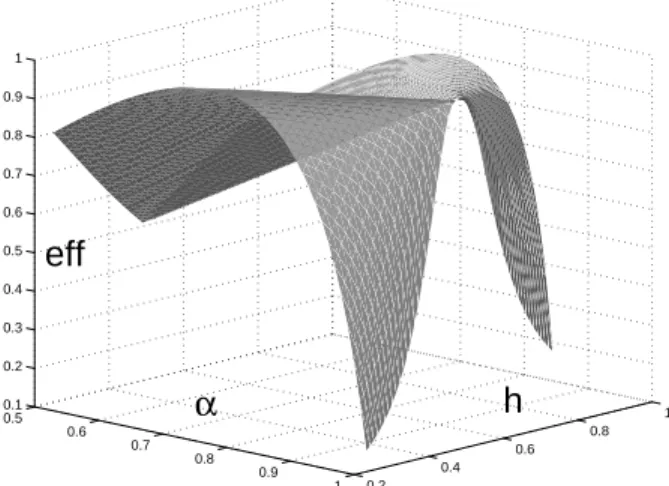
with α close to 1. Its efficiency is given by

eff(α, h) = [1, 2h]M

−1_(ξ

α∗)[1, 2h]⊤

[1, 2h]M−1_(ξ

α)[1, 2h]⊤

where α∗ _{= α}∗_{(h) corresponds to ξ}∗_{(1) in (3). The function eff(α, h) is plotted}

in Figure 1 for α _{∈ [0.5, 1), h ∈ [0.25, 0.75]. Although eff(α, 1/2) quickly}

decreases when α moves away from 1, the loss of efficiency remains reasonable

for small departures. In particular, ξ3/4 is maximin-efficient, see Silvey (1980,

p. 59): it guarantees eff(3/4, h)_{≥ 0.75 for any h ≥ 0, the minimum efficiency}

being obtained for h = 0 and h = 1/2. (Note the difference with (Schwabe,

1997) where θ1 is not restricted to be positive. The maximin-efficient design

is then ξ1/2, it is D-optimal and its minimum efficiency is 0.5.)

Another option consists in designing ξn sequentially, that is, using the

0.5 0.6 0.7 0.8 0.9 1 0.2 0.4 0.6 0.8 1 0.1 0.2 0.3 0.4 0.5 0.6 0.7 0.8 0.9 1 h α eff

Fig. 1. Efficiency eff(α, h).

of xk+1. Strong consistency of ˆθn is proved in (Ford and Silvey, 1980), ξn

converges to the optimum design ξ∗

¯

θ for ¯θ, and the asymptotic normality

√ n[h(ˆθn)_{− h(¯θ)]→ ζ}d 8 ∼ N 0, 1 4¯θ2 2 [1, 2h(¯θ)]M−(ξ_θ∗¯)[1, 2h(¯θ)]⊤ ! (13)

n → ∞, is proved in (Wu, 1985). The asymptotic efficiency thus equals one.

In particular, (13) remains valid when ¯θ1 + ¯θ2 = 0, and then coincides with

(12). When feasible, sequential design thus appears as the natural remedy to the issues raised in Sections 2 and 3. However, some difficulties should not be underestimated. The proof in (Wu, 1985) of the asymptotic result (13) under a sequential design is very much problem specific. Strong consistency of the LS estimator in the linear model under a sequential design requires

stronger conditions than M−1_(ξ

n)/n → 0, see Lai and Wei (1982). Bayesian

imbedding permits to weaken those conditions (Sternby, 1977) (at the expense

of obtaining strong consistency of the estimator for almost all values of ¯θ with

respect to some prior distribution), but its application to the sequential design of experiments (Hu, 1998) prohibits singular designs.

We hope we have convinced the reader of the richness of possible asymptotic behaviors of estimators under asymptotically singular designs. Combining this with a sequential construction of the design raises many challenging issues.

References

Buonaccorsi, J., Iyer, H., 1986. Optimal designs for ratios of linear combi-nations in the general linear model. Journal of Statistical Planning and Inference 13, 345–356.

Chaloner, K., 1989. Bayesian design for estimating the turning point of a quadratic regression. Commun. Statist.-Theory Meth. 18 (4), 1385–1400.

Fedorov, V., M¨uller, W., 1997. Another view on optimal design for estimating

the point of extremum in quadratic regression. Metrika 46, 147–157.

Ford, I., Silvey, S., 1980. A sequentially constructed design for estimating a nonlinear parametric function. Biometrika 67 (2), 381–388.

Ford, I., Titterington, D., Wu, C., 1985. Inference and sequential design. Biometrika 72 (3), 545–551.

Hu, I., 1998. On sequential designs in nonlinear problems. Biometrika 85 (2), 496–503.

Huber, P., 1973. Robust regression: asymptotics, conjectures and Monte Carlo. Annals of Statistics 1 (5), 799–821.

Lai, T., Wei, C., 1982. Least squares estimates in stochastic regression models with applications to identification and control of dynamic systems. Annals of Statistics 10 (1), 154–166.

P´azman, A., 1980. Singular experimental designs. Math. Operationsforsch. Statist., Ser. Statistics 16, 137–149.

Schwabe, R., 1997. Maximin efficient designs. Another view at D-optimality. Statistics & Probability Letters 35, 109–114.

Silvey, S., 1980. Optimal Design. Chapman & Hall, London.

Sternby, J., 1977. On consistency for the method of least squares using mar-tingale theory. IEEE Transactions on Automatic Control 22 (3), 346–352. Wu, C., 1985. Asymptotic inference from sequential design in a nonlinear

situation. Biometrika 72 (3), 553–558.

Wu, C.-F., 1980. Characterizing the consistent directions of least squares es-timates. Annals of Statistics 8 (4), 789–801.

Wynn, H., 1972. Results in the theory and construction of D-optimum exper-imental designs. Journal of Royal Statistical Society B34, 133–147.