HAL Id: hal-01564594
https://hal.archives-ouvertes.fr/hal-01564594
Submitted on 19 Jul 2017
HAL is a multi-disciplinary open access
archive for the deposit and dissemination of
sci-entific research documents, whether they are
pub-lished or not. The documents may come from
teaching and research institutions in France or
abroad, or from public or private research centers.
L’archive ouverte pluridisciplinaire HAL, est
destinée au dépôt et à la diffusion de documents
scientifiques de niveau recherche, publiés ou non,
émanant des établissements d’enseignement et de
recherche français ou étrangers, des laboratoires
publics ou privés.
A Complete Automatic Test Set Generator for
Embedded Reactive Systems: From AUTSEG V1 to
AUTSEG V2
Mariem Abdelmoula, Daniel Gaffé, Michel Auguin
To cite this version:
Mariem Abdelmoula, Daniel Gaffé, Michel Auguin. A Complete Automatic Test Set Generator for
Embedded Reactive Systems: From AUTSEG V1 to AUTSEG V2. International Journal On Advances
in Systems and Measurements, IARIA, 2016, 9 (3-4), pp.154-166. �hal-01564594�
A Complete Automatic Test Set Generator for Embedded Reactive Systems: From
AUTSEG V1 to AUTSEG V2
Mariem Abdelmoula, Daniel Gaff´e, and Michel Auguin
LEAT, University of Nice-Sophia Antipolis, CNRS Email: [email protected]
Email: [email protected] Email: [email protected]
Abstract—One of the biggest challenges in hardware and software design is to ensure that a system is error-free. Small defects in reactive embedded systems can have disastrous and costly consequences for a project. Preventing such errors by identifying the most probable cases of erratic system behavior is quite chal-lenging. Indeed, tests performed in industry are non-exhaustive, while state space analysis using formal verification in scientific research is inappropriate for large complex systems. We present in this context a new approach for generating exhaustive test sets that combines the underlying principles of the industrial testing technique with the academic-based formal verification. Our method consists in building a generic model of the system under test according to the synchronous approach. The goal is to identify the optimal preconditions for restricting the state space of the model such that test generation can take place on significant subspaces only. So, all the possible test sets are generated from the extracted subspace preconditions. Our approach exhibits a simpler and efficient quasi-flattening algorithm compared with existing techniques, and a useful compiled internal description to check security properties while minimizing the state space combinatorial explosion problem. It also provides a symbolic processing technique for numeric data that provides an expressive and concrete test of the system, while improving system verifica-tion (Determinism, Death sequences) and identifying all possible test cases. We have implemented our approach on a tool called AUTSEG V2. This testing tool is an extension of the first version AUTSEG V1 to integrate data manipulations. We present in this paper a complete description of our automatic testing approach including all features presented in AUTSEG V1 and AUTSEG V2.
Keywords–AUTSEG; Quasi-flattening; SupLDD; Backtrack; Test Sets Generation.
I. INTRODUCTION
System verification generates great interest today, espe-cially for embedded reactive systems which have complex be-haviors over time and which require long test sequences. This kind of system is increasingly dominating safety-critical do-mains, such as the nuclear industry, health insurance, banking, the chemical industry, mining, avionics and online payment, where failure could be disastrous. Preventing such failure by identifying the most probable cases of erratic system behavior is quite challenging. A practical solution in industry uses intensive test patterns in order to discover bugs, and increase confidence in the system, while researchers concentrate their efforts instead on formal verification. However, testing is obvi-ously non-exhaustive and formal verification is impracticable
on real systems because of the combinatorial explosion nature of the state space.
AUTSEG V1 [2] combines these two approaches to provide an automatic test set generator, where formal verification ensures automation in all phases of design, execution and test evaluation and fosters confidence in the consistency and relevance of the tests. In a first version of AUTSEG, only Boolean inputs and outputs were supported, while most of actual systems handle numerical data. Numerical data ma-nipulation represents a big challenge for most of existing test generation tools due to the difficulty to express formal properties on those data using a concise representation. In our approach, we consider symbolic test sets which are thereby more expressive, safer and less complex than the concrete ones. Therefore, we have developed a second version AUTSEG V2 [1] to take into account numerical data manipulation in addition to Boolean data manipulation. This was achieved by developing a new library for data manipulation called SupLDD. Prior automatic test set generation methods have been consequently extended and adapted to this new numer-ical context. Symbolic data manipulations in AUTSEG V2 allow not only symbolic data calculations, but also system verification (Determinism, Death sequences), and identification of all possible test cases without requiring coverage of all system states and transitions. Hence, our approach bypasses in numerous cases the state space explosion problem.
We present in this paper a complete description of our auto-matic testing approach that includes all operations introduced in AUTSEG V1 and AUTSEG V2. In the remainder of this paper, we give an overview of related work in Section II. We present in Section III our global approach to test generation. A case study is presented in Section IV. We show in Section V experimental results. Finally, we conclude the paper in Section VI with some directions for future works.
II. RELATEDWORK
Lutess V2 [3] is a test environment, written in Lustre, for synchronous reactive systems. It automatically generates tests that dynamically feed the program under test from the formal description of the program environment and properties. This version of Lutess deals with numeric inputs and outputs unlike the first version [4]. Lutess V2 is based on Constraint Logic Programming (CLP) and allows the introduction of hypotheses
to the program under test. Due to CLP solvers’ capabilities, it is possible to associate occurrence probabilities to any Boolean expression. However, this tool requires the conversion of tested models to the Lustre format, which may cause a few issues in our tests.
B. Blanc presents in [5] a structural testing tool called GATeL, also based on CLP. GATeL aims to find a sequence that satisfies both the invariant and the test purpose by solving the constraints problem on program variables. Contrary to Lutess, GATeL interprets the Lustre code and starts from the final state and ends with the first one. This technique relies on human intervention, which is stringently averted in our paper. C. Jard and T. Jeron, present TGV (Test Generation with Verification technology) in [6], a powerful tool for test gener-ation from various specificgener-ations of reactive systems. It takes as inputs a specification and a test purpose in IOLTS (Input Output Labeled Transition System) format and generates test cases in IOLTS format as well. TGV allows three basic types of operations: First, it identifies sequences of the specifica-tion accepted by a test purpose, based on the synchronous product. It then computes visible actions from abstraction and determination. Finally, it selects test cases by computation of reachable states from initial states and co-reachable states from accepting states. A limitation lies in the non-symbolic (enumerative) dealing with data. The resulting test cases can be big and therefore relatively difficult to understand.
D. Clarke extends this work in [7], presenting a symbolic test generation tool called STG. It adds the symbolic treatment of data by using OMEGA tool capabilities. Test cases are therefore smaller and more readable than those done with enumerative approaches in TGV. STG produces the test cases from an IOSTS specification (Input Output Symbolic Transi-tion System) and a test purpose. Despite its effectiveness, this tool is no longer maintained.
STS (Symbolic Transition Systems) [8] is quite often used in systems testing. It enhances readability and abstraction of behavioral descriptions compared to formalisms with limited data types. STS also addresses the states explosion problem through the use of guards and typed parameters related to the transitions. At the moment, STS hierarchy does not appear very enlightening outside the world of timed/hybrid systems or well-structured systems. Such systems are outside of the scope of this paper.
ISTA (Integration and System Test Automation) [9] is an interesting tool for automated test code generation from High-Level Petri Nets. ISTA generates executable test code from MID (Model Implementation Description) specifications. Petri net elements are then mapped to implementation constructs. ISTA can be efficient for security testing when Petri nets gen-erate threat sequences. However, it focuses solely on liveness properties checking, while we focus on security properties checking.
J. Burnim presents in [10], a testing tool for C called CREST. It inserts instrumentation code using CIL (C Interme-diate Language) into a target program. Symbolic execution is therefore performed concurrently with the concrete execution. Path constraints are then solved using the YICES solver. CREST currently reasons symbolically only about linear, in-teger arithmetic. Closely related to CREST, KLOVER [11] is a symbolic execution and automatic test generation tool for
C++ programs. It basically presents an efficient and usable tool to handle industrial applications. Both KLOVER and CREST cannot be adopted in our approach, as they accommodate tests on real systems, whereas we target tests on systems still being designed.
III. ARCHITECTURALTESTOVERVIEW
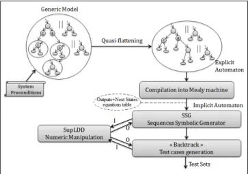
We introduce in this section the principles of our automatic testing approach including data manipulation. Fig .1 shows five main operations including: i) the design of a global model of the system under test, ii) a quasi-flattening operation, iii) a compilation process, iv) a generation process of symbolic sequences mainly related to the symbolic data manipulation entity, v) and finally the backtrack operation to generate all possible test cases.
Figure 1. Global Test Process.
1. Global model: it presents the main input of our test. The global architecture is composed of hierarchical and parallel concurrent FSM based on the synchronous approach. It should conform to the specification of the system under test.
2. Quasi-flattening process: it flattens only hierarchical automata while maintaining parallelism. This offers a simple model, faster compilation, and brings more flexibility to iden-tify all possible system evolutions.
3. Compilation process: it generates an implicit automaton represented by a Mealy machine from an explicit automaton. This process compiles the model, checks the determinism of all automata and ensures the persistence of the system behavior.
4. Symbolic data manipulation (SupLDD): it offers a sym-bolic means to characterize system preconditions by numerical constraints. It is solely based on the potency of the LDD library [4]. The symbolic representation of these preconditions shows an important role in the subsequent operations for generating symbolic sequences and performing test cases ”Backtrack”. It evenly enhances system security by analyzing the constraints computations.
5. Sequences Symbolic Generation (SSG): it works locally on significant subspaces. It automatically extracts necessary preconditions which lead to specific, significant states of the system from generated sequences. It relies on the effective representation of the global model and the robustness of numerical data processing to generate the exhaustive list of
possible sequences, avoiding therefore the manual and explicit presentation of all possible combinations of system commands. 6. Backtrack operation: it allows the verification of the whole system behavior through the manipulation of extracted preconditions from each significant subspace. It verifies the execution context of each significant subspace. Specifically, it identifies all paths satisfying each final critical state precondi-tions to reach the root state.
A. Global model
In this paper, we particularly focus on verification of embedded software controlling reactive systems behavior. The design of such systems is generally based on the synchronous approach [12] that presents clear semantics to exceptions, delays and actions suspension. This notably reduces the pro-gramming complexity and favors the application of verification methods. In this context, we present the global model by hierarchical and parallel concurrent Finite States Machines (FSMs) based on the synchronous approach. The hierarchical machine describes the global system behavior, while parallel automata act as observers for control data of the hierarchical automaton. Our approach allows for testing many types of systems at once. In fact, we present a single generic model for all types of systems, the specification of tests can be done later using particular Boolean variables called system preconditions (type of system, system mode, etc.). Hence, a specific test generation could be done at the end of test process through analysis of the system preconditions. This prevents generating as many models as system types, which can highly limit the legibility and increase the risk of specification bugs.
B. Quasi-flattening process
A straightforward way to analyze a hierarchical machine is to flatten it first (by recursively substituting in a hierarchical FSM, each super state with its associated FSM and calculating the Cartesian product of parallel sub-graphs), then apply on the resulting FSM a verification tool such as a model-checking or a test tool. We will show in our approach that we don’t need to apply the Cartesian product, we can flatten only hierarchical automata: This is why we call it ”Quasi-flattening”.
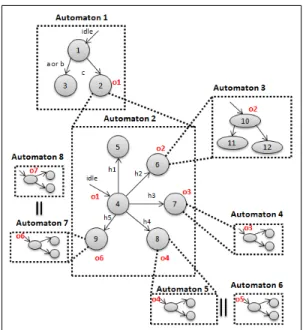
Let us consider the model shown in Fig .2, which shows automata interacting and communicating between each other. Most of them are sequential, hierarchical automata (e.g. au-tomata 1 and 2), while others are parallel auau-tomata (e.g. automata 6 and 8). We note in this architecture 13122 (3 × 6 × 3 × 3 × 3 × 3 × 3 × 3) possible states derived from parallel executions (graphs product) while there are many fewer reachable states at once. This model is designed by the graphic form of Light Esterel language [13]. This language is inspired by SyncCharts [14] in its graphic form, Esterel [15] in its textual form and Lustre [16] in its equational form. It integrates high-level concepts of synchronous languages in an expressive graphical formalism (taking into account the concept of multiple events, guaranteeing the determinism, providing a clear interpretation, rationally integrating the pre-emption concept, etc.).
A classical analysis is to transform this hierarchical struc-ture in Light Esterel to the synchronous language Esterel. Such a transformation is not quite optimized. In fact, Esterel is not able to realize that there is only one active state at once. In practice, compiling such a structure using Esterel generates 83
Figure 2. Model Design.
registers making roughly 9.6 ×1024 states. Hence, the behoof of our process. Opting for a quasi-flattening, we have flattened only hierarchical automata, while the global structure remained parallel. Thus, state 2 of automaton 1 in Fig .2 is substituted by the set of states {4, 5, 6, 7, 8, 9} of automaton 2 and so on. Required transitions are rewritten thereafter. Parallel automata are acting as observers that manage the model’s control flags. Flattening parallel FSMs explode usually in terms of number of states. Thus there is no need to flatten them, as we can compile them separately thanks to the synchronous approach, then concatenate them with the flat model retrieved at the end of the compilation process. This quasi-flattening operation allows for flattening the hierarchical automata and maintaining the parallelism. This offers a simpler model, faster compilation, and brings more flexibility to identify all possible evolutions of the system as detailed in the following steps.
Algorithm 1 details our quasi-flattening operation. We denote downstream the initial state of a transition and upstream the final one. This algorithm implements three main operations. Overall, it replaces each macro state with its associated FSM. It first interconnects the internal initial states. It then replaces normal terminations (Refers to SyncCharts ”normal termina-tion” transition [14]) with internal transitions in a recursive manner. Finally, it interconnects all states of the internal FSM.
Figure 3. Interconnection of Internal States.
We show in Fig .3 the operation of linking internal initial states described in lines 3 to 9 of algorithm 1. This latter starts
Algorithm 1 Flattening operation
1: St ← State; SL ← State List of FSM; t ← transition in FSM
2: while (SL 6= empty) do 3: Consider each St from SL
4: if (St is associated to a sub-FSM) then 5: mark the deletion of St
6: load all sub-St from sub-FSM (particularly init-sub-St)
7: for (all t of FSM) do
8: if (upstream(t) == St) then
9: upstream(t) ← init-sub-St // illustration in Fig .3 (t0, t1, t2 relinking)
10: for (all t of FSM) do
11: if (downstream(t) == St) then
12: if (t is a normal-term transition) then 13: // illustration in Fig .4
14: for (all sub-St of sub-FSM) do
15: if (sub-St is associated to a sub-sub-FSM) then
16: create t0 (sub-St, upstream(t)) // Keep recursion
17: if (sub-St is final) then 18: for (all t00 of sub-FSM) do
19: if (upstream(t00) == sub-St) then 20: upstream(t00) ← upstream(t); merge
effect(t) to effect(t00) 21: else
22: // weak or strong transition: illustration in Fig .3
23: // For example t3 is less prior than t6 and replaced by t6.t3 and t6
24: for (all sub-St of sub-FSM) do 25: if (t is a weak transition) then
26: create t0(sub-St,upstream(t),trigger(t), weak-effect(t))
27: else
28: create t0(sub-St,upstream(t),trigger(t)) 29: for (all sub-t of sub-FSM) do
30: turn-down the sub-t priority (or turn up t0 priority)
31: delete t
by marking the super state St to load it in a list and to be deleted later. Then, it considers all associated states sub-St(states 3, 4, 5). For each transition in the global automaton, if the upstream state of this transition is the super state St, then this transition will be interconnected to the transition of the initial state of St (state 3). This corresponds to relinking t0, t1, t2.
Fig .4 illustrates the connection of a normal termination transition (lines 10 to 20 of algorithm 1). If the downstream state of a normal termination transition (t5) is a super state St, then the associated sub-states (1,2,3,4) are considered. If these sub-states are super states too, then a connection is created between these states and the upstream state of the normal termination transition.
Otherwise, if these sub-states are final states (3,4), then they will be merged with the upstream state of the normal termination transition (state 5). Finally, the outputs of the
Figure 4. Normal Transition Connection.
merged states are redirected to the resulted state. St is marked in a list to be deleted at the end of the algorithm.
Besides, in case of a weak or a strong preemption transition (According to SyncCharts and Esterel: in case of weak pre-emption, preempted outputs are emitted a last time, contrary to the strong preemption), we create transitions between all sub-states of the super state St and their upstream states, as described in lines 21 to 31 of algorithm 1. Fig .3 illustrates this step, where t6 and t7 are considered to be preemption transitions: all the internal states (3,4,5) of the super state St are connected to their upstream states (6,7). Then, the priority of transitions is managed: the upper level transitions are prior to those of lower levels. In this context, t3 is replaced by t7.t6.t3 to show that t6 and t7 are prior than t3 and so on. At the end of this algorithm, all marked statements are deleted. In case of weak preemption transition, the associated outputs are transferred to the new transitions.
Flattening the hierarchical model of Fig .2 results in a flat structure shown in Fig .5. As the activation of state 2 is a trigger for state 4, these two states will be merged, just as state 6 will be merged to state 10, etc. Automata 6 and 8 (observers) remain parallel in the expanded automaton; they are small and do not increase the computational complexity. The model in Fig .5 contains now only 144 (16 × 3 × 3) state combinations. In practice, compiling this model according to our process generates merely 8 registers, equivalent to 256 states.
Figure 5. Flat Model.
Our flattening differs substantially from those of [17] and [18]. We assume that a transition, unlike the case of the states diagram in Statecharts, cannot exit from different hierarchical levels. Several operations are thus executed locally, not on the global system. This yields a simpler algorithm and faster compilation. To this end, we have integrated the following assumptions in our algorithm:
-Normal termination. Fig .4 shows an example of normal termination carried when a final internal state is reached. It allows a unique possible interpretation and facilitates code generation.
-Strong preemption. Unlike the weak preemption, internal outputs of the preempted state are lost during the transition.
C. Compilation process
We proceed in our approach to a symbolic compilation of the global model into Mealy machines, implicitly represented by a set of Boolean equations (circuit of logic gates and registers presenting the state of the system). In fact, the flat automata and concurrent automata are compiled separately. Compilation results of these automata are concatenated at the end of this process. They are represented by a union of sorted equations rather than a Cartesian product of graphs to support the synchronous parallel operation and instantaneous diffusion of signals as required by the synchronous approach. Accordingly, the system model is substantially reduced. Our compilation requires only log2(nbstates) registers, while
clas-sical works uses one register per state [19]. It also allows checking the determinism of all automata, which ensures the persistence of the system behavior.
Algorithm 2 describes the compilation process in details. First, it counts the number of states in the automaton and deduces the size of the states vector. Then, it develops the function of the next state for a given state variable. Finally, the generated vector is characterized by a set of Boolean expressions. It is represented by a set of BDDs.
Let us consider an automaton with 16 states as an exam-ple. The vector characterizing the next state is created by 4 (log2(16)) expressions derived from inputs data and the current
state. For each transition from state ”k” to state ”l”, two types of vectors encoded by n (n = 4 bits in this example) bits are created: Vk vector specifying the characteristic function of
transition BDDcond, and Vlvector characterizing the function
of the future state BDD − N extState. If Vk(i) is valued to 1,
then the state variable yi is considered positively. Otherwise,
yi is reversed (lines 18-22). In this context, the BDD
charac-terizing the transition condition is deduced by the combination of ”yi” and the condition ”cond” on transition. For instance,
BDDcond= y0× ¯y1× ¯y2× y3× cond for Vk = (1, 0, 0, 1).
We show in lines (23-27) the construction of the Next State function BDD − N extState(i) = BDDy(i)+ ×
notBDDy(i)0 +. BDDy(i)+ characterizes all transitions that
turns yi+ to 1 (Set registers to 1). Conversely, BDDy(i)0 +
characterizes all transitions that turns yi+ to 0 (Reset registers to 0). So, each function satisfying y+ and not (y0+) is a possible solution. In this case, parsing all states of the system is not necessary. Fig .6 shows an example restricted to only 2 states variables where it is possible to find an appropriate function ”BDD+y1 respect = y0.x + y0.x” for y+1 and ”BDD+y0 respect = y0.x + y1.y0.x” for y+0 even
if the system state is not specified for ”y1y0 = 11”.Thus,
BDD − N extState (BDDy(i)+) is specified by the two
BDDrespect looking for the simplest expressions to check
on one hand y0+ and not(y00+) and on the other hand y+1 and not(y01+).
Algorithm 2 Compilation process 1: R ← Vector of states
2: R-I ← Initial vector of states (initial value of registers) 3: Next-State ← Vector of transitions
4: N ← Size of R and Next-State 5: f,f’ ← Vectors of Boolean functions 6: N ← log2(Statesnumber − 1)+ 1
7: Define N registers encapsulated in R. 8: for (i=0 to N − 1) do
9: BDDf (i) ← BDD-0 // BDD initialisation
10: BDDf0(i) ← BDD-0
11: for (j=0 to N outputs − 1) do 12: OutputO(j) ← BDD-0
13: R-I ← binary coding of initial state 14: for (transition tkl=k to l) do 15: Vk ← Binary coding of k 16: Vl← Binary coding of l 17: BDDcond ← cond (tkl); 18: for (i=0 to N − 1) do 19: if Vk(i)==1 then
20: BDDcond ← BDDand(R(i), BDDcond ) //
BDDcond: tkl BDD characteristics
21: else
22: BDDcond ← BDDand(BDDnot (R(i)),
BDDcond)
23: if (Vl(i)==1) then
24: BDDf (i) ← BDDor(BDDf (i), BDDcond )//
BDDf (i): set of register
25: else
26: BDDf0(i) ← BDDor(BDDf0(i), BDDcond))//
BDDf0(i): reset of register
27: outputO(output(tkl))← BDDor
(outputO(output(tkl)), BDDcond)
28: for (i=0 to N − 1) do
29: BDD-NextState(i)← BDDrespect(BDDf, BDD0f)
30: // respect: every BDDh such us BDDf → BDDh
AND BDDh → not(BDD0f)
Figure 6. Next State Function.
As we handle automata with numerical and Boolean vari-ables, each data inequation was first replaced by a Boolean variable (abstraction). Then at the end of the compilation process, data were re-injected to be processed by SupLDD later.
D. Symbolic data manipulation
In addition to Boolean functions, our approach allows numerical data manipulation. This provides more expressive and concrete system tests.
1) Related work: Since 1986, Binary Decision Diagrams (BDDs) have successfully emerged to represent Boolean func-tions for formal verification of systems with large state space. BDDs, however, cannot represent quantitative information such as integers and real numbers. Variations of BDDs have been proposed thereafter to support symbolic data manipulations that are required for verification and performance analysis of systems with numeric variables. For example, Multi-Terminal Binary Decision Diagrams (MTBDDs) [20] are a generaliza-tion of BDDs in which there can be multiple terminal nodes, each labelled by an arbitrary value. However, the size of nodes in an MTBDD can be exponential (2n) for systems with large ranges of values. To support a larger number of values, Yung-Te Lai has developed Edge-Valued Binary Decision Diagrams (EVBDDs) [21] as an alternative to MTBDDs to offer a more compact form. EVBDDs associate multiplicative weights with the true edges of an EVBDD function graph to allow an optimal sharing of subgraphs. This suggests a linear evolution of non-terminal node sizes rather than an exponential one for MTBDDs. However, EVBDDs are limited to relatively simple calculation units, such as adders and comparators, implying a high cost per node for complex calculations such as (X × Y ) or (2X).
To overcome this exponential growth, Binary Moment Diagrams (BMDs) [22], another variation of BDDs, have been specifically developed for arithmetic functions considered to be linear functions, with Boolean inputs and integer outputs, to perform a compact representation of integer encodings and operations. They integrate a moment decomposition principle giving way to two sub-functions representing the two moments (constant and linear) of the function, instead of a decision. This representation was later extended to Multiplicative Bi-nary Moment Diagrams (*BMDs) [23] to include weights on edges, allowing to share common sub-expressions. These edges’ weights are multiplicatively combined in a *BMD, in contrast to the principle of addition in an EVBDD. Thus, the following arithmetic functions X + Y , X − Y , X × Y , 2X
show representations of linear size. Despite their significant success in several cases, handling edges’ weights in BMDs and *BMDs is a costly task. Moreover, BMDs are unable to verify the satisfiability property, and function outputs are non-divisible integers in order to separate bits, causing a problem for applications with output bit analysis. BMDs and MTBDDs were combined by Clarke and Zhao in Hybrid Decision Diagrams (HDDs) [24]. However, all of these diagrams are restricted to hardware arithmetic circuit checking and are not suitable for the verification of software system specifications. Within the same context of arithmetic circuit checking, Taylor Expansion Diagrams (TEDs) [25] have been introduced to supply a new formalism for multi-value polynomial func-tions, providing a more abstract, standard and compact design representation, with integer or discrete input and output values. For an optimal fixed order of variables, the resulting graph is canonical and reduced. Unlike the above data structures, TED is defined on a non-binary tree. In other words, the number of child nodes depends on the degree of the relevant variable. This makes TED a complex data structure for particular
functions such as (ax). In addition, the representation of the
function (x < y) is an important issue in TED. This is particularly challenging for the verification of most software system specifications. In this context, Decision Diagrams for Difference logic (DDDs) [26] have been proposed to present functions of first order logic by inequalities of the form {x − y ≤ c} or {x − y < c} with integer or real variables. The key idea is to present these logical formulas as BDD nodes labelled with atomic predicates. For a fixed variables order, a DDD representing a formula f is no larger than a BDD of a propositional abstraction of f. It supports as well dynamic programming by integrating an algorithm called QELIM, based on Fourier-Motzkin elimination [27]. Despite their proved efficiency in verifying timed systems [28], the difference logic in DDDs is too restrictive in many program analysis tasks. Even more, dynamic variable ordering (DVO) is not supported in DDDs. To address those limitations, LDDs [29] extend DDDs to full Linear Arithmetic by supporting an efficient scheduling algorithm and a QELIM quantification. They are BDDs with non-terminal nodes labelled by linear atomic predicates, satisfying a scheduling theory and local constraints reduction. Data structures in LDDs are optimally ordered and reduced by considering the many implications of all atomic predicates. LDDs have the possibility of computing arguments that are not fully reduced or canonical for most LDD operations. This suggests the use of various reduction heuristics that trade off reduction potency for calculation cost. 2) SupLDD: We summarize from the above data structures that LDD is the most relevant work for data manipulation in our context. Accordingly, we have developed a new library called Superior Linear Decision Diagrams (SupLDD) built on top of Linear Decision Diagrams (LDD) library. Fig .7 shows an example of representation in SupLDD of the arithmetic formula F 1 = {(x ≥ 5) ∧ (y ≥ 10) ∧ (x + y ≥ 25)} ∨ {(x < 5)∧(z > 3)}. Nodes of this structure are labelled by the linear predicates {(x < 5); (y < 10); (x + y < 25); (−z < −3)} of formula F1, where the right branch evaluates its predicates to 1 and the left branch evaluates its predicates to 0. In fact, the choice of a particular comparison operator within the 4 possi-ble operators {<, ≤, >, ≥} is not important since the 3 other operators can always be expressed from the chosen operator: {x < y} ⇔ {N EG(x ≥ y)}; {x < y} ⇔ {−x > −y} and {x < y} ⇔ {N EG(−x ≤ −y)}.
Figure 7. Representation in SupLDD of F1.
We show in Fig .7.b that the representation of F1 in SupLDD has the same structure as a representation in BDD that labels its nodes by the corresponding Boolean variables
{C0; C1; C2; C3} to each SupLDD predicate. But, a repre-sentation in SupLDD is more advantageous. In particular, it ensures the numerical data evaluation and manipulation of all predicates along the decision diagram. This furnishes a more accurate and expressive representation in Fig .7.c than the original BDD representation. Namely, the Boolean variable C3 is replaced by EC3 which evaluates the corresponding node to {x+y < 15} instead of {x+y < 25} taking into account prior predicates {x < 5} and {y < 10}. Besides, SupLDD relies on an efficient T-atomic scheduling algorithm [29] that makes compact and non-redundant diagrams for SupLDD where a node labelled for example by {x ≤ 15} never appears as a right child of a node labelled by {x ≤ 10}. As well, nodes are ordered by a set of atoms {x, y, etc.} where a node labelled by {y < 2} never appears between two nodes labelled by {x < 0} and {x < 13}. Further, SupLDD diagrams are optimally reduced, including the LDD reduction rules. First, the QELIM quantification introduced in LDDs allows the elimination of multiples variables: For example, the QELIM quantification of the expression {(x−y ≤ 3)∧(x−t ≥ 8)∧(y−z ≤ 6)∧(t−k ≥ 2)} eliminates the intermediate variables y and t and generates the simplified expression {(x − z ≤ 9) ∧ (x − k ≥ 10)}. Second, the LDD high implication [29] rule enables getting the smallest geometric space: For example, simplifying the expression {(x ≤ 3) ∧ (x ≤ 8)} in high implication yields the single term {x ≤ 3}. Finally, the LDD low implication [29] rule generates the largest geometric space where the expression {(x ≤ 3) ∧ (x ≤ 8)} becomes {x ≤ 8}.
SupLDD operations- SupLDD operations are primarily generated from basic LDD operations [29]. They are simpler and more adapted to our needs. We present functions to manip-ulate inequalities of the form {P aixi ≤ c}; {P aixi < c};
{P aixi ≥ c}; {P aixi > c}; where {ai, xi, c ∈ Z}. Given
two inequalities I1 and I2, the main operations in SupLDD
include:
-SupLDD conjunction (I1, I2): This absolutely corresponds to the intersection on Z of subspaces representing I1 and I2.
-SupLDD disjunction (I1, I2): As well, this operation abso-lutely corresponds to the union on Z of subspaces representing I1 and I2.
Accordingly, all the space Z can be represented by a union of two inequalities {x ≤ a} ∪ {x > a}. As well, the empty set can be inferred from the intersection of inequalities {x ≤ a} ∩ {x > a}.
-Equality operator {P aixi= c}: It is defined by the
inter-section of two inequalities {P aixi ≤ c} and {P aixi≥ c}.
-Resolution operator: It simplifies arithmetic expressions using QELIM quantification, and both low and high implica-tion rules introduced in LDD. For example, the QELIM reso-lution of {(x−y ≤ 3)∧(x−t ≥ 8)∧(y −z ≤ 6)∧(x−t ≥ 2)} gives the simplified expression {(x − z ≤ 9) ∧ (x − t ≥ 8) ∧ (x − t ≥ 2)}. This expression can be further simplified to {(x − z ≤ 9) ∧ (x − t ≥ 8)} in case of high implication and to {(x − z ≤ 9) ∧ (x − t ≥ 2)} in case of low implication.
-Reduction operator: It solves an expression A with respect to an expression B. In other words, if A implies B, then the reduction of A with respect to B is the projection of A when B is true. For example, the projection of A {(x − y ≤ 5) ∧ (z ≥ 2) ∧ (z − t ≤ 2)} with respect to B {x − y ≤ 7} gives the reduced set {(z ≥ 2) ∧ (z − t ≤ 2)}.
We report in this paper on the performance of these functions to enhance our tests. More specifically, by means of the SupLDD library, we present next the Sequences Symbolic Generation operation that integrates data manipulation and generates more significant and expressive sequences. More-over, we track and analyze test execution to spot the situations where the program violates its properties (Determinism, Death sequences). On the other hand, our library ensures the analysis of the generated sequences context to carry the backtrack operation and generate all possible test cases.
E. Sequences Symbolic Generation (SSG)
Contrary to the classical sequences generator that follows only one of the possible paths, we proceed to a symbolic execution [30] to automatically explore all possible paths of the studied system. The idea is to manipulate logical formulas matching interrelated variables instead of updating directly the variables in memory, in the case of concrete classical execution. Fig .8 presents a set of possible sequences describing the behavior of a given system. It is a classical representation of the dynamic system evolutions. It shows a very large tree or even an infinite tree. Accordingly, exploring all possible program executions is not at all feasible. This requires imagining all possible combinations of the system commands, which is almost impossible. We will show in the next session the weakness of this classical approach when testing large systems.
Figure 8. Classical Sequences Generation.
If we consider the representation of the system by a sequence of commands executed iteratively, the previous se-quences tree becomes a repetition of the same subspace pattern as shown in Fig .9. Instead of considering all the state space, we seek in our approach to restrict the state space and confine only on significant subspaces. This represents a specific system command, which can be repeated through possible generated sequences. Each state in the subspace is specified by 3 main variables: symbolic values of the program variables, path condition and command parameters (next byte-code to be executed). The path condition represents preconditions that should be satisfied by the symbolic values to successfully advance the current path execution.
Figure 9. AUTSEG Model Representation.
In other words, it defines the preconditions to successfully follow that path. We particularly define two types of precon-ditions:
• Boolean global preconditions that define the execution context of a given command. They appear as input constraints of the tested command. They state the list of commands that should be executed beforehand. They arise as well as command output if the latter is properly executed.
• Numerical local preconditions that define numerical constraints on commands parameters. They are pre-sented and manipulated by SupLDD functions men-tioned in Section III-D2. Thus, they are presented in the form of {P aixi ≤ c}; {P aixi < c};
{P aixi ≥ c}; {P aixi > c}; where xi presents the
several commands parameters.
Our approach is primarily designed to test systems running iterative commands. In this context, the SSG operation occurs in the significant subspace representing a system command instead of considering all the state space. It generates the ex-haustive list of possible sequences in each significant subspace and extracts the optimal preconditions defining its execution context. In fact, we test all system commands, but a single command is tested at once. The restriction was done by characterizing all preconditions defining the execution context in each subspace. Hence, the major complex calculation is intended to be locally performed in each significant subspace avoiding the state space combinatorial explosion problem.
Indeed, the safety of the tested system is checked by means of SupLDD analysis on numerical local preconditions and BDD analysis on Boolean global preconditions. First, we check if there are erroneous sequences. To this end, we apply the SupLDD conjunction function on all extracted numerical preconditions within the analyzed path. If the result of this conjunction is null, the analyzed sequence is then impossible and should be rectified! Second, we check the determinism of the system behavior. To this end, we verify if the SupLDD conjunction of all outgoing transitions from each state is empty. In other words, we verify if the SupLDD disjunction of all outgoing transitions from each state is equal to all of the space covering all possible system behaviors. Finally, we check the execution context of each command. This is to identify and verify that all extracted global preconditions are met. If the context is verified, then the generated sequence is considered safe. This verification operation is performed by the ”Backtrack” operation detailed below.
Algorithm 3 shows in detail the symbolic sequences gen-eration opgen-eration executed in each subspace. This allows auto-matically generating all possible sequences in a command and extract its global pre-conditions. This operation is quite simple because it relies on the flexibility of the designed model, compiled through the synchronous approach. We have applied symbolic analysis (Boolean via BDD-analysis and numeric via SupLDDs) from the local initial state (initial state of the com-mand) to local final states of the specified subspace. For each combination of registers, BDD and SupLDD manipulations are applied to determine and characterize the next state and update the state variables. Required preconditions for this transition are identified as well. If these preconditions are global, then they are inserted into the GPLIST of global preconditions to be displayed later in the context of the generated sequence. Otherwise, if these preconditions are local, then they are pushed into a stack LPLIST, in conjunction with the previous ones. If the result of this conjunction is null, then the generated sequence is marked impossible and should be rectified. Outputs are calculated as well and pushed into a stack OLIST. Finally, the sequence is completed by the new established state. Once the necessary global preconditions are extracted, a next step is to backtrack the tree until the initial sequence fulfilling these preconditions is found.
Algorithm 3 SSG operation 1: Seq ← sequence 2: BDS ← BDD State 3: BDA ← BDD awaited
4: BDAC ← BDD awaited context 5: OLIST ← Outputs list
6: GPLIST ← Global Precondition list 7: LPLIST ← Local Precondition list 8: BDS ← Initial state
9: BDAC ← 0 10: OLIST ← empty 11: GPLIST ← empty 12: LPLIST ← All the space 13: Push (BDS, OLIST, BDAC) 14: while (stack is not empty) do 15: Pull (BDS, OLIST, BDAC)
16: list(BDA)← Compute the BDD awaited expressions list(BDS)
17: for (i=0 to |list(BDA)|) do 18: Input ← extract(BDA)
19: if (Input is a global precondition) then 20: GPLIST ← Push(GPLIST, Input) 21: else
22: if (Input is a local precondition) then 23: LPLIST ← SupLDD-AND(LPLIST, Input) 24: if (GPLIST is null) then
25: Display ( Impossible Sequence !) 26: Break
27: NextBDS ← Compute future(BDS, BDA) 28: OLIST ← Compute output (BDS, BDA) 29: New-seq ← seq BDA | BDA
30: if (New New-seq size < maximum diameter) then 31: Push (NextBDS, OLIST, BDAC)
32: else
33: Display (GPLIST) 34: Display (New-seq)
F. Backtrack operation
Once the necessary preconditions are extracted, the next step consists in backtracking paths from each final critical state toward the initial state, finding the sequence fulfilling these preconditions. This operation is carried by robust calculations on SupLDD and the compilation process, which kept enough knowledge to find later the previous states (Predecessors) that lead to the initial state. Algorithm 4 details this operation in two main phases: The first one (lines 11-20) labels the state space nodes, which are not yet analyzed. From the initial state (e ← 0), all successors are labelled by (e ← e + 1). If a state is already labelled, its index is not incremented. This operation is repeated for all states until the whole state space is covered. The second phase (lines 21-30) identifies the best previous states. For each state St, the predecessor with the lowest label is introduced into the shortest path to reach the initial state: This is an important result of graph theory [31]. In other words, previous states always converge to the same global initial state. This approach easily favors the backtracking execution. Algorithm 4 Search for Predecessors
1: St ← State
2: LSt ← List of States 3: LS ← List of Successors 4: LabS ← State Label 5: IS ← Initial State 6: S ← State 7: LabS(IS) ← 1 8: LSt ← IS
9: LP ← List of Predecessors 10: SMin ← Minimum Lab State 11: // Expansion 12: while (LSt != 0) do 13: for (all St of LSt) do 14: LS ← Get-Successors(St) 15: if (LS != 0) then 16: for (all S of LS) do 17: if (!LabS(S)) then 18: LabS(S) ← LabS(St)+1 19: NLSt ← Push(LS) 20: LSt ← NLSt
21: // Search for Predecessors 22: for (all St) do
23: LP ← Get-Predecessor(St) 24: SMin ← LabS(first(LP)) 25: StMin ← first(LP) 26: for (all St’ in LP) do
27: if (LabS(St’) < SMin) then 28: SMin ← LabS(St’) 29: StMin ← St’
30: Memorise-Backtrack(St,StMin)
Let us consider the example in Fig .9. From the initial local state ”IL” (initial state of a command), the symbolic sequences generator applies BDDs and SupLDDs analysis to generate all possible paths that lead to final local states of the tested subspace. Taking into account ”LF” as a critical final state ”FS” of the tested system, the backtrack operation is executed from ”LF” state until the sequence that satisfies the extracted global preconditions. Assuming state ”I” as the final result of
this backtrack, the sequence from ”I” to ”LF” is an example of a good test set. However, considering the representation of Fig .8, a test set from ”I” to ”LF” will be performed by generating all paths of the tree. Such a test becomes unfeasible if the number of steps to reach ”LF” is greatly increased. The Backtrack operation includes two main actions:
- Global backtrack: It verifies the execution context of the tested subspace. It is based on Boolean global preconditions to identify the list of commands that should be executed before the tested command.
- Local backtrack: Once the list of commands is estab-lished, a next step is to execute a local backtrack. It determines the final path connecting all commands to be executed to reach the specified final state. It uses numeric local preconditions of each command from the list.
Fig .10 details the global backtrack operation: Given the global extracted preconditions (GP1, GP2, etc.) from the SSG operation at this level (Final state FS of command C1), we search in the global actions table for actions (Commands C2 and C3) that emit each parsed global precondition. Next, we put on a list SL the states that trigger each identified action (SL= {C2, C3}). This operation is iteratively executed on all found states (C2,C3) until the root state I with zero preconditions (C4 with zero preconditions) is reached.
Figure 10. Global Backtrack.
The identified states can be repeated on SL (C2 and C4 are repeated on SL) as many times as there are commands that share the same global preconditions (C1 and C3 share the same precondition GP1). To manage this redundancy, we allocate a priority P to each found state, where each state of priority P should precede the state of priority P+1. More specifically, if an identified state already exists in SL, then its priority is incremented by 1 (Priority of commands C2 and C4 are incremented by 1). By the end of this operation, we obtain the list SL (SL= { C3,C2,C4 }) of final states referring to subspaces that should be traced to reach I.
A next step is to execute a local backtrack on each identified subspace (C1,C3,C2,C4), starting from the state with the lowest priority and so on to trace the final path from FS to I. The sequence from I to FS is an example of a good test set. Fig .11 presents an example of local backtracking in command C3. In fact, during the SSG operation each state S was labelled by (1) a Local numeric Precondition (LP)
Figure 11. Local Backtrack.
presenting numerical constraints that should be satisfied on its ongoing transition and (2) a Total Local numeric precondition (TL) that presents the conjunction of all LP along the executed path from I to S. To execute the local backtrack, we start from the ongoing transition PT to FS to find a path that satisfies the backtrack precondition BP initially defined by TL. If the backtrack precondition is satisfied by the total precondition {T L ≥ BP }, then if the local precondition LP of the tested transition is not null, we remove this verified precondition LP from BP by applying the SupLDD projection function. Next, we move to the amount state of PT and test its ongoing transitions, etc. However, if {T L < BP }, we move to the test of other ongoing transitions to find the transition from which BPcan be satisfied. This operation is iteratively executed until reaching the initial state on which the backtrack precondition is null (fully satisfied). In short, if the context is verified, the generated sequence is considered correct. At the end of this process, we join all identified paths from each traced subspace according to the given priority order from the global backtrack operation.
IV. USECASE
To illustrate our approach, we studied the case of a contact-less smart card for the transportation sector manufactured by the company ASK [32], a world leader in this technology. We specifically targeted the verification of the card’s functionality and security features. Security of such systems is critical: it can concern cards for access security, banking, ID, etc. Card complexity makes it difficult for a human to identify all possible delicate situations, or to validate them by classical methods. We need approximately 500 000 years to test the first 8 bytes if we consider a classical Intel processor able to generate 1000 test sets per second. As well, combinatorial explosion of possible modes of operation makes it nearly impossible to attempt a comprehensive simulation. The prob-lem is exacerbated when the system integrates numerical data processing. We will show in the next session the results of applying our tool to this transportation card, taking into account the complexity of data manipulation. We compared
our testing approach to that of ASK. We also compared our results to those obtained with a classical approach.
The smart card operation is defined by a transport standard called Calypso that presents 33 commands. The succession of these commands (e.g., Open Session, SV Debit, Get Data, Change Pin) gives the possible scenarios of card operation. We used Light Esterel [13] to interpret the card specification (Calypso) into hierarchical automata while taking advantages of this synchronous language. We designed the generic model of the studied card by 52 interconnected automata including 765 states. Forty-three of them form a hierarchical structure. The remaining automata operate in parallel and act as ob-servers to control the global context of hierarchical automaton (Closed Session, Verified PIN, etc.). We show in Fig .12 a small part of our model representing the command Open Session. Each command in Calypso is presented by an APDU (Application Protocol Data Unit) that presents the next byte-code to be executed (CLA,INS,P1,P2, etc.). We expressed these parameters by SupLDD local preconditions on various transitions. For instance, AUTSEGINT(h10 < P 1 < h1E) means that the corresponding transition can only be executed if (10 < P 1 < 30). Autseg-Open-Session and Back-Autseg-Verify-PIN are examples of global preconditions that appear as outputs of respectively Open Session and Verify PIN commands when they are correctly executed. They appear also as inputs for other commands as SV Debit command to denote that the card can be debited only if the PIN code is correct and a session is already open.
Figure 12. Open Session Command.
According to the Calypso standard, several card types and configurations are defined (contact/contactless, with/without Stored-Value, etc.). Typically, these characteristics must be initially configured to specify each test. However, changing card parameters requires recompiling each new specification separately and re-running the tests. This approach is
un-realistic, because this can take many hours or even days to compile in industry. In addition, this would generate as many models as system types, which can highly limit the legibility and increase the risk of specification bugs. Contrary to this complex testing process, our approach yields a single appropriate generic model for all card types and applications. The model’s explicit test sets are to be filtered at the end of the test process through analysis of system preconditions. For instance, Autseg-Contact-mode is an example of a system precondition specifying that Open Session command should be executed in a Contactless Mode. In this context, checking a contactless card involves evaluating Autseg-Contact-mode to 0 and then verifying the corresponding execution context. Accordingly, sequences with the precondition Autseg-Contact-mode are false and should be rectified!
V. EXPERIMENTALRESULTS
In this section, we show experimental results of applying our tool to the contactless transportation card. We intend to test the security of all possible combinations of 33 commands of the Calypso standard. This validation process is extremely important to determine whether the card performs to specifi-cation. Each command in the Calypso standard is encoded on a minimum of 8 bytes. We conducted our experiments on a PC with an Intel Dual Core GHz Processor, 8 GB RAM.
We have achieved a vast reduction of the state space due to the quasi-flattening process on the smart card hierarchical model. Compared to classical flattening works, we have moved from 9.6 1024 states in the designed model to only 256 per
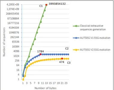
branch of parallel. Then, due to the compilation process, we have moved from 477 registers to only 22. More impressive results are obtained on sequences generation and test coverage with data processing. A classical test of this card can be achieved by browsing all paths of the tree in Fig .13 without any restriction. This tree represents all possible combinations of 33 commands of the Calypso standard.
Figure 13. Classical Test of Calypso Card.
Such a test shows in plot C1 of Fig .14 an exponential evolution of the number of sequences versus the number of tested bytes. We are not even able to test just a simple sequence of two commands. Our model explodes by 13 bytes generating
3,993,854,132 possible sequences. That’s why AUTSEG tests only one command at once, but it introduces a notion of preconditions and behavior backtracking to abstract the effects of the previous commands in the sequence under test.
Figure 14. SSG Evolutions.
Hence, a second test applies AUTSEG V1 (without data processing) on the card model represented in the same manner as Fig .9. It generates all possible paths in each significant subspace (command) separately. Results show in plot C2 a lower evolution that stabilizes at 10 steps and 1784 paths, allowing for coverage of all states of the tested model. More interesting results are shown in plot C3 by AUTSEG V2 tests taking into account numerical data manipulation. Our approach enables coverage of the global model in a substantially short time (a few seconds). It allows separately testing 33 commands (all of the system commands) in only 21 steps, generating a total of solely 474 paths. Covering all states in only 21 steps, our results demonstrate that we test separately one command (8 bytes) at once in our approach thanks to the backtrack operation. The additional steps (13 bytes) correspond to the test of system preconditions (e.g., AUTSEG-Contact-mode, etc.), global preconditions (e.g., Back-Autseg-Open-Session, etc.) and other local preconditions (e.g.,AUTSEGINT(h00 ≤ buf f er−size ≤ hF F )). Whereas, only fewer additional steps (2 bytes) are required within the first version of AUTSEG that stabilizes at 10 steps. This difference proves a complete handling of system constraints using the new version of AUTSEG, performing therefore more expressive and real tests: we integrate a better knowledge of the system.
Plot C4 in Fig .15 exhibits results of AUTSEG V2 tests simulated with 3 anomalies on the smart card model. We note fewer generated sequences by the 5 steps. We obtain a total of 460 sequences instead of 474 at the end of the tests. Fourteen sequences are removed since they are unfea-sible (dead sequences) according to SupLDD calculations. Indeed, the SupLDD conjunction of parsed local precondi-tions AUTSEGINT(01h ≤ RecordN umber ≤ 31h) and AUTSEGINT(RecordN umber ≥ F F h) within a same path is null, illustrating an over-specification example (anomaly) of the Calypso standard that should be revised.
Figure 15. AUTSEG V2 SSG Evolutions.
We show in Fig .16 an excerpt of generated sequences by AUTSEG V2 detecting another type of anomaly: an under-specification in the card behavior. The Incomplete Behavior message reports a missing action on a tested state of the Update-Binary command. Indeed, two actions are defined (T ag = 54h) and (T ag = 03h) at this state. All states where Tag is different from 84 and 3 are missing. We can automatically spot such problems by checking for each parsed state if the union of all outgoing transitions is equal to the whole space. If this property is always true, then the smart card behavior is proved deterministic.
Figure 16. Smart Card Under-Specification.
As explained before, we get the execution context of each generated sequence at the end of this operation. The next step is then to backtrack all critical states of the Calypso standard (all final states of 33 commands). Fig .17 shows a detailed example of backtracking from the final state of the SV Undebit command that emits SW6200 code. We identify from the global extracted preconditions Back-Autseg-Open-Session and Back-Autseg-Get-SV the list of commands (Open Secure Session and SV Get) to be executed beforehand. Then, we look recursively for all global preconditions of each identified command to trace the complete path to the initial state of
Figure 17. SV Undebit Backtrack.
the Start command. We observe from the results that the Verify PIN command should proceed the Open Secure Session command. So, the final backtrack path is to trace (local backtrack) the identified commands respectively SV Undebit, SV Get, Open Secure Session and Verify PIN using local preconditions of each command. At the end of this process, we generate automatically 5456 test sets that cover the entire behavior of the studied smart card.
Figure 18. Tests Coverage.
Industry techniques, on the other hand, take much more time to manually generate a mere 520 test sets, covering 9,5% of our tests as shown in Fig .18.
VI. CONCLUSION
We have proposed a complete automatic testing tool for embedded reactive systems that details all features presented in our previous works AUTSEG V1 and AUTSEG V2. Our testing approach focused on systems executing iterative com-mands. It is practical and performs well, even with large models where the risk of combinatorial explosion of state space is important. This has been achieved by essentially (1) exploiting the robustness of synchronous languages to design an effective system model easy to analyze, (2) providing an algorithm to quasi-flatten hierarchical FSMs and reduce the state space, (3) focusing on pertinent subspaces and restricting the tests, and (4) carrying out rigorous calculations to generate an exhaustive list of possible test cases. Our experiments
confirm that our tool provides expressive and significant tests, covering all possible system evolutions in a short time. More generally, our tool including the SupLDD calculations can be applied to many numerical systems as they could be modelled by FSMs handling integer variables. Since SupLDD is imple-mented on top of a simple BDD package, we aim in a future work to rebuild SupLDD on top of an efficient implementation of BDDs with complement edges [33] to achieve a better library optimization. More generally, new algorithms can be integrated to enhance the LDD library. We aim as well to integrate SupLDD in data abstraction of CLEM [13]. More details about these future works are presented in [34]. Another interesting contribution would be to generate penetration tests to determine whether a system is vulnerable to an attack.
REFERENCES
[1] M. Abdelmoula, D. Gaff´e, and M. Auguin, “Automatic Test Set Gen-erator with Numeric Constraints Abstraction for Embedded Reactive Systems: AUTSEG V2,” in VALID 2015: The Seventh International Conference on Advances in System Testing and Validation Lifecycle, Barcelone, Spain, Nov. 2015, pp. 23–30.
[2] M. Abdelmoula, D. Gaff´e, and M. Auguin, “Autseg: Automatic test set generator for embedded reactive systems,” in Testing Software and Systems, 26th IFIP International Conference,ICTSS, ser. Lecture Notes in Computer Science. Madrid, Spain: springer, September 2014, pp. 97–112.
[3] B. Seljimi and I. Parissis, “Automatic generation of test data generators for synchronous programs: Lutess v2,” in Workshop on Domain specific approaches to software test automation: in conjunction with the 6th ESEC/FSE joint meeting, ser. DOSTA ’07. New York, NY, USA: ACM, 2007, pp. 8–12.
[4] L. DuBousquet and N. Zuanon, “An overview of lutess: A specification-based tool for testing synchronous software,” in ASE, 1999, pp. 208– 215.
[5] B. Blanc, C. Junke, B. Marre, P. Le Gall, and O. Andrieu, “Handling state-machines specifications with gatel,” Electron. Notes Theor. Comput. Sci., vol. 264, no. 3, 2010, pp. 3–17. [Online]. Available: http://dx.doi.org/10.1016/j.entcs.2010.12.011 [Accessed 15 November 2016]
[6] J. R. Calam, “Specification-Based Test Generation With TGV,” CWI, CWI Technical Report SEN-R 0508, 2005. [Online]. Available: http://oai.cwi.nl/oai/asset/10948/10948D.pdf [Accessed 15 November 2016]
[7] D. Clarke, T. J´eron, V. Rusu, and E. Zinovieva, “Stg: A symbolic test generation tool,” in TACAS, 2002, pp. 470–475.
[8] L. Bentakouk, P. Poizat, and F. Za¨ıdi, “A formal framework for service orchestration testing based on symbolic transition systems,” Testing of Software and Communication Systems, 2009.
[9] D. Xu, “A tool for automated test code generation from high-level petri nets,” in Proceedings of the 32nd international conference on Applications and theory of Petri Nets, ser. PETRI NETS’11. Berlin, Heidelberg: Springer-Verlag, 2011, pp. 308–317.
[10] J. Burnim and K. Sen, “Heuristics for scalable dynamic test generation,” in Proceedings of the 2008 23rd IEEE/ACM International Conference on Automated Software Engineering, ser. ASE ’08. Washington, DC, USA: IEEE Computer Society, 2008, pp. 443–446.
[11] G. Li, I. Ghosh, and S. P. Rajan, “Klover: a symbolic execution and automatic test generation tool for c++ programs,” in Proceedings of the 23rd international conference on Computer aided verification, ser. CAV’11. Berlin, Heidelberg: Springer-Verlag, 2011, pp. 609–615. [12] C. Andr´e, “A synchronous approach to reactive system design,” in 12th
EAEEIE Annual Conf., Nancy (F), May 2001, pp. 349–353. [13] A. Ressouche, D. Gaff´e, and V. Roy, “Modular compilation of a
synchronous language,” in Soft. Eng. Research, Management and Ap-plications, best 17 paper selection of the SERA’08 conference, R. Lee, Ed., vol. 150. Prague: Springer-Verlag, August 2008, pp. 157–171.
[14] C. Andr´e, “Representation and analysis of reactive behaviors: A syn-chronous approach,” in Computational Engineering in Systems Appli-cations (CESA). Lille (F): IEEE-SMC, July 1996, pp. 19–29. [15] G. Berry and G. Gonthier, “The esterel synchronous programming
language: Design, semantics, implementation,” Sci. Comput. Program., vol. 19, no. 2, Nov. 1992, pp. 87–152. [Online]. Available: http://dx.doi.org/10.1016/0167-6423(92)90005-V [Accessed 15 November 2016]
[16] N. Halbwachs, P. Caspi, P. Raymond, and D. Pilaud, “The synchronous dataflow programming language lustre,” in Proceedings of the IEEE, 1991, pp. 1305–1320.
[17] A. C. R. Paiva, N. Tillmann, J. C. P. Faria, and R. F. A. M. Vidal, “Modeling and testing hierarchical guis,” in Proc.ASM05. Universite de Paris 12, 2005, pp. 8–11.
[18] A. Wasowski, “Flattening statecharts without explosions,” SIGPLAN Not., vol. 39, no. 7, Jun 2004, pp. 257–266. [Online]. Available: http://doi.acm.org/10.1145/998300.997200 [Accessed 15 November 2016]
[19] I. Chiuchisan, A. D. Potorac, and A. Garaur, “Finite state machine design and vhdl coding techniques,” in 10th International Conference on development and application systems. Suceava, Romania: Faculty of Electrical Engineering and Computer Science, 2010, pp. 273–278. [20] M. Fujita, P. C. McGeer, and J. C.-Y. Yang, “Multi-terminal binary
decision diagrams: An efficient datastructure for matrix representation,” Form. Methods Syst. Des., vol. 10, no. 2-3, Apr. 1997, pp. 149–169. [21] Y.-T. Lai and S. Sastry, “Edge-valued binary decision diagrams
for multi-level hierarchical verification,” in Proceedings of the 29th ACM/IEEE Design Automation Conference, ser. DAC’92. Los Alami-tos, CA, USA: IEEE Computer Society Press, 1992, pp. 608–613. [22] R. E. Bryant and Y.-A. Chen, “Verification of arithmetic circuits
with binary moment diagrams,” in Proceedings of the 32Nd Annual ACM/IEEE Design Automation Conference, ser. DAC ’95. New York, NY, USA: ACM, 1995, pp. 535–541.
[23] L. Arditi, “A bit-vector algebra for binary moment diagrams,” I3S, Sophia-Antipolis, France, Tech. Rep. RR 95–68, 1995.
[24] E. Clarke and X. Zhao, “Word level symbolic model checking: A new approach for verifying arithmetic circuits,” Pittsburgh, PA, USA, Tech. Rep., 1995.
[25] M. Ciesielski, P. Kalla, and S. Askar, “Taylor expansion diagrams: A canonical representation for verification of data flow designs,” IEEE Transactions on Computers, vol. 55, no. 9, 2006, pp. 1188–1201. [26] J. Møller and J. Lichtenberg, “Difference decision diagrams,” Master’s
thesis, Department of Information Technology, Technical University of Denmark, Building 344, DK-2800 Lyngby, Denmark, Aug. 1998. [27] A. J. C. Bik and H. A. G. Wijshoff, Implementation of Fourier-Motzkin
Elimination. Rijksuniversiteit Leiden. Valgroep Informatica, 1994. [28] P. Bouyer, S. Haddad, and P.-A. Reynier, “Timed petri nets and
timed automata: On the discriminating power of zeno sequences,” Inf. Comput., vol. 206, no. 1, Jan. 2008, pp. 73–107.
[29] S. Chaki, A. Gurfinkel, and O. Strichman, “Decision diagrams for linear arithmetic.” in FMCAD. IEEE, 2009, pp. 53–60.
[30] R. S. Boyer, B. Elspas, and K. N. Levitt, “Select a formal system for testing and debugging programs by symbolic execution,” SIGPLAN Not., vol. 10, no. 6, Apr. 1975, pp. 234–245. [Online]. Available: http://doi.acm.org/10.1145/390016.808445 [Accessed 15 November 2016]
[31] D. B. Johnson, “A note on dijkstra’s shortest path algorithm,” J. ACM, vol. 20, no. 3, Jul. 1973, pp. 385–388. [Online]. Available: http://doi.acm.org/10.1145/321765.321768 [Accessed 15 November 2016]
[32] “Ask.” [Online]. Available: http://www.ask-rfid.com/ [Accessed 15 November 2016]
[33] K. Brace, R. Rudell, and R. Bryant, “Efficient implementation of a bdd package,” in Design Automation Conference, 1990. Proceedings., 27th ACM/IEEE, June 1990, pp. 40–45.
[34] M. Abdelmoula, “Automatic test set generator with numeric constraints abstraction for embedded reactive systems,” Ph.D. dissertation, Pub-lished in ”G´en´eration automatique de jeux de tests avec analyse sym-bolique des donn´ees pour les syst`emes embarqu´es”, Sophia Antipolis University, France, 2014.