Interglacial instability of North Atlantic Deep Water ventilation

HAL Id: hal-02968727

https://hal.archives-ouvertes.fr/hal-02968727

Submitted on 7 Dec 2020

HAL is a multi-disciplinary open access

archive for the deposit and dissemination of sci-entific research documents, whether they are pub-lished or not. The documents may come from teaching and research institutions in France or abroad, or from public or private research centers.

L’archive ouverte pluridisciplinaire HAL, est destinée au dépôt et à la diffusion de documents scientifiques de niveau recherche, publiés ou non, émanant des établissements d’enseignement et de recherche français ou étrangers, des laboratoires publics ou privés.

ventilation

Eirik Vinje Galaasen, Ulysses Ninnemann, Augustin Kessler, Nil Irvalı, Yair

Rosenthal, Jerry Tjiputra, Nathaëlle Bouttes, Didier Roche, Helga (kikki) F.

Kleiven, David Hodell

To cite this version:

Eirik Vinje Galaasen, Ulysses Ninnemann, Augustin Kessler, Nil Irvalı, Yair Rosenthal, et al.. Inter-glacial instability of North Atlantic Deep Water ventilation. Science, American Association for the Advancement of Science, 2020, 367 (6485), pp.1485-1489. �10.1126/science.aay6381�. �hal-02968727�

1

Title: Interglacial instability of North Atlantic Deep Water ventilation

1

Authors: Eirik Vinje Galaasen1*, Ulysses S. Ninnemann1, Augustin Kessler2,Nil Irvalı1, Yair

2

Rosenthal3, Jerry Tjiputra2, Nathaëlle Bouttes4, Didier M. Roche4,5, Helga (Kikki) F. Kleiven1,

3

David A. Hodell6

4

Affiliations:

5

1_{Department of Earth Science and Bjerknes Centre for Climate Research, University of Bergen,}

6

Bergen, Norway.

7

2_{NORCE Norwegian Research Centre, Bjerknes Centre for Climate Research, Bergen,}

8

Norway.

9

3_{Institute of Marine and Coastal Sciences and Department of Earth and Planetary Sciences,}

10

Rutgers University, New Brunswick, NJ, USA.

11

4_{Laboratoire des Sciences du Climat et de l’Environnement, LSCE/IPSL, CEA-CNRS-UVSQ,}

12

Université Paris-Saclay, Gif-sur-Yvette, France.

13

5_{Vrije Universiteit Amsterdam, Faculty of Science, Cluster Earth and Climate, Amsterdam,}

14

The Netherlands.

15

6_{Godwin Laboratory for Paleoclimate Research, Department of Earth Sciences, University of}

16

Cambridge, Cambridge, UK.

17

*Correspondence to: [email protected]

18 19

Abstract: Disrupting North Atlantic Deep Water (NADW) ventilation is a key concern in

20

climate projections. We use (sub-)centennially resolved bottom water δ13C records spanning

21

the interglacials of the last 0.5 million years to assess the frequency and climatic backgrounds

22

capable of triggering large NADW reductions. Episodes of reduced NADW in the deep

23

Atlantic, similar in magnitude to glacial events, have been relatively common and occasionally

24

long-lasting features of interglacials. Critically, NADW reductions were triggered across the

25

range of recent interglacial climate backgrounds, demonstrating that catastrophic freshwater

26

outburst floods were not a prerequisite for large perturbations. Our results argue that large

27

NADW disruptions are more easily achieved than previously appreciated and occurred in past

28

climate conditions similar to those we may soon face.

2

One Sentence Summary: Large and frequent changes in ocean ventilation during recent warm

30

periods question its modern stability.

31

Main Text: Atlantic meridional overturning circulation (AMOC) and North Atlantic Deep

32

Water (NADW) ventilation represents a low probability, high impact tipping point (1) in the

33

climate system with implications for the distribution and sequestration of anthropogenic CO2

34

and heat, and for Atlantic-wide patterns of climate and sea level (2-4). While the consequences

35

of any changes are clearly severe, the probability for instabilities in the rate or pathways of

36

NADW ventilation remains highly uncertain. Simple and complex models both suggest large

37

changes are possible, but also that a strong overturning like that found in the modern ocean

38

may be more difficult to disrupt than an overall weaker circulation (4-6). Likewise, most

39

models simulate moderate to no reduction in AMOC in response to future source region

40

buoyancy increases (1) but may be biased towards stability (7) and struggle to reproduce the

41

rich spectrum of variability revealed by a decade of observations (8, 9). Testing these physical

42

and conceptual models, and more generally the stability of NADW ventilation in warm

43

climates, requires empirical constraints from beyond the current state of circulation.

44

Given a background climate similar to today, the modern mode of deep Atlantic

45

ventilation with strong NADW influence (Fig. 1) appears stable on long multi-millennial

46

timescales. Proxy reconstructions indicate that modern NADW ventilation pathways persisted

47

with little multi-millennial variability in recent interglacial periods (10-14). By contrast,

48

pronounced AMOC variability has occurred on timescales of a decade or less in observations

49

(8, 9) suggesting strong mean overturning is comprised of significant variance. However, little

50

is known about NADW variability on the intermediary timescales, leaving the variability

51

within a long-term ‘vigorous’ mean ventilation state poorly defined. There are few proxy

3

reconstructions depicting higher-frequency variability and those available are largely confined

53

to the last two interglacials, the Holocene and Marine Isotope Stage (MIS) 5e. During these

54

periods, the largest changes in deep Atlantic ventilation involving reductions of NADW

55

influence occurred on relatively short centennial timescales and were focused around intervals

56

with wasting of continental ice sheet remnants from the preceding glaciation (10, 12, 15). This

57

includes the century-long NADW reduction at 8.2 thousand years (ky) before present (B.P.)

58

following the freshwater outburst flood from glacial Lake Agassiz (12). Absence of similarly

59

large changes in the last ~eight ky of the Holocene (e.g., 12) has supported the notion of

60

vigorous and stable ventilation as generally representative of interglacial boundary conditions.

61

Beyond the last two interglacials, little is known about centennial-scale variability in

62

NADW, despite its relevance for delimiting the natural variability of ocean ventilation and the

63

frequency of large NADW reductions under different background climates. The most recent

64

interglacials MIS 5e, 7e, 9e, and 11c are particularly relevant, as these periods had similar

65

climate boundary conditions to the current MIS 1 in addition to episodes of high-latitude

66

warming, Greenland Ice Sheet (GrIS) retreat, and sea level rise relative to the modern (16-18).

67

This offers an opportunity to test the robustness of NADW ventilation under source region

68

conditions similar to those projected for the future (1). Here we reconstruct northwest Atlantic

69

bottom water δ13C to trace NADW influence (Fig. 1) over MIS 7e, 9e, and 11c and provide a

70

detailed perspective on NADW ventilation instability during recent interglacials.

71

Our epibenthic foraminifera Cibicidoides wuellerstorfi (sensu stricto) δ13C record (19)

72

from International Ocean Drilling Program (IODP) Site U1305 (57°29’N, 48°32’W; 3459 m

73

water depth) at the Eirik Drift is situated to monitor lower NADW entering the deep Atlantic

74

(Fig. 1). Due to the potential for uncertainty in δ13C reconstructions (e.g., 20), we only consider

4

changes in the running mean of three samples (averaging five data points; see (19)) and signals

76

outside the standard error of data within this window to reflect bottom water δ13C variability,

77

which, given negligible influence from organic carbon fluxes (21), provides a proxy for past

78

changes in the ventilation and distribution of water masses (e.g., 20, 22). The Eirik Drift

79

bottom water δ13C record indicates large changes in deep Atlantic carbon chemistry during the

80

interglacial δ18O plateaus of MIS 7e, 9e, and 11c (Fig. 2). Each interglacial contained abrupt

81

changes in bottom water δ13C as large (≤1.0‰) as those of the bordering glacial terminations

82

and inceptions (Fig. 2), and similar to those occurring after freshwater outburst floods such as

83

the ~8.2 ky B.P. event (12) and during MIS 5e (10). Absolute values range from near modern

84

NADW levels (≥0.8‰; Fig. 1) to those typical of the glacial deep Atlantic (13, 14, 23, 24).

85

While similar in magnitude, the frequency, timing, and duration of these changes differ among

86

individual interglacial periods. Low bottom water δ13C values persist for a millennium or more

87

during late MIS 7e (~233.5-243.5 ky; on our age model, 19) and mid- to late MIS 9e

(~323.0-88

326.0 ky), whereas large (~0.5‰) multi-centennial variability punctuated MIS 11c

89

superimposed on multi-millennial trends.

90

Low bottom water δ13C values at Site U1305 likely reflect reduced NADW influence

91

and changes in deep Atlantic ventilation patterns. Reduced (high-δ13C) NADW influence and

92

incursions of (low-δ13C) Southern source water (SSW) explain many features of the observed

93

variability, including the: 1) spatial consistency of intermittently low δ13C observed at different

94

deep sites (Site U1304 and U1305; Fig. 3); 2) abruptness of the δ13C changes as the

NADW-95

SSW water mass boundary shifted across the core sites; 3) shift of Site U1305 δ13C towards the

96

millennially averaged values found near the northern or the southern source regions (Fig. 3);

5

and 4) association of high (low) C. wuellerstorfi δ13C with high (low) C. wuellerstorfi B/Ca in

98

selected Eirik Drift samples (Fig. S6) (19).

99

We further use a transient interglacial (115-125 ky) simulation (19) with the

isotope-100

enabled intermediate complexity iLOVECLIM Earth system model (25) to assess potential

101

links between variability in deep Atlantic δ13C, NADW distribution, and AMOC. Simulated

102

centennial-scale episodes of NADW shoaling and SSW expansion produce δ13C reductions in

103

the deep Atlantic that strongly match the magnitude, rate and duration of the variability

104

observed in our (Fig. 4) and other reconstructions (e.g., 10, 12-14) consistent with the inference

105

that the δ13C variability reflect changes in NADW distribution. These large deep Atlantic δ13C

106

changes, which are similar in magnitude to glacial millennial-scale changes (e.g., 23, 24), were

107

achieved without a total collapse of but with a significant (~16 to ~8 Sv) decrease in AMOC

108

strength and accompanied by cooling in the subpolar North Atlantic (Fig. 4).

109

Our results call for reconsideration of the long-held notion of warm-climate stability in

110

deep Atlantic carbon chemistry and ventilation. This view of stability likely remains true for

111

the (multi-)millennial mean state, as previously depicted by lower-resolution records lacking

112

the fidelity to resolve the shorter timescale that is characteristic of NADW reductions (Fig. 3).

113

High-resolution records are naturally biased towards the youngest strata and the current

114

interglacial, the Holocene. Yet, when contextualized against the late Pleistocene interglacials,

115

the Holocene stands out as having had the most stable lower NADW ventilation of the last half

116

million years (Fig. 3), which was only strongly curtailed at ~8.2 ky B.P. (12). Bottom water

117

δ13C and NADW reductions similar to that at ~8.2 ky B.P. were prevalent features of prior

118

interglacials, occasionally even lasting millennia (Fig. 3). Ventilation patterns changed

119

repeatedly from one similar to the modern (Fig. 1) to one with reduced NADW and incursions

6

of SSW in the deep North Atlantic (~3.4 km), similar to that illustrated by our model

121

simulation (Fig. 4).

122

The short duration of interglacial NADW reductions may indicate a change in the

123

intrinsic ocean dynamics operating under different background climate states. The interglacial

124

deep Atlantic is clearly better ventilated than the glacial on long equilibrium timescales (11, 13,

125

14, 23, 24). However, the magnitude of ventilation pattern changes that are possible appears

126

similar in (de-)glacial (e.g., 11, 24, 26) and interglacial periods when variability in lower

127

NADW is considered at shorter timescales (Fig. 3). The centennial-scale duration and transient

128

nature of most interglacial NADW reductions (Fig. 3; Fig. 4) suggests the modern ventilation

129

pattern tends to recover quickly when perturbed, and is similar to the AMOC recovery

130

timescale seen in many numerical models forced with buoyancy increases (e.g., 4). With this in

131

mind, the longer-lasting NADW reductions in MIS 7e (~233.5-234.5 ky), 9e (~323-326 ky),

132

and late 11c (~401-408 ky) either required more sustained forcing or suggests that the recovery

133

timescale following perturbations is not fixed. Most interglacial NADW reductions were still

134

short-lived compared to those associated with glacial (Dansgaard-Oeschger) variability (e.g.,

135

24), suggesting either that NADW ventilation behaved differently or the persistence of any

136

forcing changed, depending on the climate state. One possible explanation for this timescale

137

difference is the extensive glacial expansion of high-latitude sea ice, which could promote a

138

baseline increase in SSW ventilation (27) and prolong the duration of northern ventilation

139

anomalies (28). A lack of strong sea ice responses could also explain the potentially muted

140

climate variability in interglacial compared to glacial climates (10, 13, 14, 29), despite the

141

presence of NADW variability. More high-resolution climate records spanning past

142

interglacials are however needed to conclusively evaluate the impacts of warm-climate NADW

7

reductions, and delineate its role relative feedbacks such as sea ice responses in driving

144

interglacial climate variability.

145

Model simulations suggest future warming and freshwater addition from an intensified

146

hydrological cycle and ice sheet melting could all increase source region buoyancy and curtail

147

convective NADW renewal (1, 4). The common occurrence of NADW reductions in past

148

interglacials (Fig. 3) clearly demonstrates the potential for large changes in deep Atlantic

149

ventilation and allows us to explore the triggers for perturbations. NADW reductions during

150

the last two interglacial periods were confined mainly to the early warm interglacial phases,

151

concurrent with high northern hemisphere summer insolation and known freshwater outburst

152

floods accompanying the final retreat of residual glacial ice sheets (Fig. 3) (10, 12, 30, 31).

153

While stratigraphically belonging to interglacial periods, to the extent that these anomalies are

154

related to wasting vestiges of glaciation, they are likely best viewed mechanistically as the final

155

episodes of deglaciation. By contrast, NADW reductions in MIS 7e, 9e, and 11c occurred in

156

the mid and late interglacial phases under low summer insolation (Fig. 3) and after any likely

157

deglacial freshwater influences. This implies that NADW reductions can occur without the

158

excess buoyancy input provided by wasting residual glacial ice sheets, or the influence of large

159

continental ice sheets on atmospheric circulation. Ice sheet activity may still have played a role

160

in regulating the stability of NADW ventilation during some periods. NADW reductions in

161

MIS 7e, 9e, and 11c often coincided with, or were preceded by, input of ice-rafted debris (IRD)

162

at Site U1305 (Fig. 3), indicating supply of icebergs and freshwater proximal to the NADW

163

source region. Furthermore, the prolonged NADW reduction of MIS 9e was associated with

164

elevated southern GrIS sediment discharge and MIS 1 stability with low GrIS activity (32),

165

while particularly strong GrIS retreat in MIS 11c (16, 18) occurred alongside persistent NADW

8

variability (Fig. 3). These observations are consistent with ice sheet activity and freshwater

167

addition intermittently influencing the formation or downstream density of lower NADW.

168

However, variability in NADW ventilation, IRD input, and GrIS discharge also occurred

169

independently of each other (Fig. 3), implicating additional controls on NADW ventilation and

170

supporting models suggesting convective instability is possible with relatively small buoyancy

171

input if delivered to the convection regions (e.g., 6).

172

Our results suggest we should consider rapid and large changes in NADW ventilation

173

not only as a possibility (10, 12, 30) but even as an intrinsic feature of centennial-scale

174

variability in warm climate states. This has implications for constraining the potential for and

175

cause of change in the modern Atlantic. First, it supports concerns that disregarding large

176

variability in simulations may have biased future AMOC projections towards stability (7). The

177

possibility of large natural variability on decadal (8, 9) to centennial timescales (Fig. 3) also

178

complicates attribution of variability in the deep Atlantic, but the characteristics of this

179

variability may be used to differentiate between natural and anthropogenic change in the

180

coming century. While past changes were predominantly multi-centennial, there are also

181

climate and ocean conditions that can drive longer NADW reductions, as evidenced for

182

example by the ~3000 years-long anomaly in mid-MIS 9e (Fig. 3). Specifically what these

183

conditions were remains unclear, but the triggers for NADW instability have clearly operated

184

across the range of recent interglacial climate conditions. Recognizing this requires moving

185

beyond the notion of vigorous and stable deep Atlantic ventilation as representative of warm

186

climate states (e.g., 1, 5, 11), and towards conceptual and numerical models that can account

187

for pronounced variability across various timescales and climate states.

188 189

9 References and Notes:

190

1. IPCC, in Climate Change 2013: The Physical Science Basis. Contribution of Working

191

Group I to the Fifth Assessment Report of the Intergovernmental Panel on Climate

192

Change, T. F. Stocker et al., Eds., Summary for Policymakers (Cambridge Univ. Press,

193

Cambridge, United Kingdom and New York, NY, USA, 2013).

194

2. M. W. Buckley, J. Marshall, Observations, inferences, and mechanisms of the Atlantic

195

Meridional Overturning Circulation: A review. Reviews of Geophysics 54, 5-63 (2016).

196

3. C. L. Sabine et al., The oceanic sink for anthropogenic CO2. Science 305, 367-371

197

(2004).

198

4. T. F. Stocker, A. Schmittner, Influence of CO2 emission rates on the stability of the

199

thermohaline circulation. Nature 388, 862-865 (1997).

200

5. H. Stommel, Thermohaline convection with two stable regimes of flow. Tellus 13,

224-201

230 (1961).

202

6. T. F. Stocker, D. G. Wright, Rapid transitions of the ocean's deep circulation induced

203

by changes in surface water fluxes. Nature 351, 729-732 (1991).

204

7. M. Hofmann, S. Rahmstorf, On the stability of the Atlantic meridional overturning

205

circulation. Proc. Natl. Acad. Sci. U.S.A. 106, 20584-20589 (2009).

206

8. M. Srokosz, H. Bryden, Observing the Atlantic Meridional Overturning Circulation

207

yields a decade of inevitable surprises. Science 348, 1255575 (2015).

208

9. M. Lozier et al., A sea change in our view of overturning in the subpolar North

209

Atlantic. Science 363, 516-521 (2019).

210

10. E. V. Galaasen et al., Rapid Reductions in North Atlantic Deep Water During the Peak

211

of the Last Interglacial Period. Science 343, 1129-1132 (2014).

10

11. J. F. Adkins, E. A. Boyle, L. Keigwin, E. Cortijo, Variability of the North Atlantic

213

thermohaline circulation during the last interglacial period. Nature 390, 154-156

214

(1997).

215

12. H. K. F. Kleiven et al., Reduced North Atlantic Deep Water coeval with the glacial

216

Lake Agassiz freshwater outburst. Science 319, 60-64 (2008).

217

13. J. F. McManus, D. W. Oppo, J. L. Cullen, A 0.5-million-year record of millennial-scale

218

climate variability in the North Atlantic. Science 283, 971-975 (1999).

219

14. D. W. Oppo, J. F. McManus, J. L. Cullen, Abrupt climate events 500,000 to 340,000

220

years ago: Evidence from subpolar North Atlantic sediments. Science 279, 1335-1338

221

(1998).

222

15. D. A. Hodell et al., Surface and deep-water hydrography on Gardar Drift (Iceland

223

Basin) during the last interglacial period. Earth Planet. Sci. Lett. 288, 10-19 (2009).

224

16. A. de Vernal, C. Hillaire-Marcel, Natural variability of Greenland climate, vegetation,

225

and ice volume during the past million years. Science 320, 1622-1625 (2008).

226

17. A. Berger et al., Interglacials of the last 800,000 years. Reviews of Geophysics 54,

162-227

219 (2016).

228

18. A. V. Reyes et al., South Greenland ice-sheet collapse during Marine Isotope Stage 11.

229

Nature 510, 525-528 (2014).

230

19. See the supplementary materials.

231

20. A. Schmittner et al., Calibration of the carbon isotope composition (δ13C) of benthic

232

foraminifera. Paleoceanography 32, 512-530 (2017).

11

21. B. Corliss, X. Sun, C. Brown, W. Showers, Influence of seasonal primary productivity

234

on δ13C of North Atlantic deep-sea benthic foraminifera. Deep Sea Research Part I:

235

Oceanographic Research Papers 53, 740-746 (2006).

236

22. M. Eide, A. Olsen, U. S. Ninnemann, T. Johannessen, A global ocean climatology of

237

preindustrial and modern ocean δ13C. Global Biogeochem. Cycles 31, 515-534 (2017).

238

23. L. E. Lisiecki, M. E. Raymo, W. B. Curry, Atlantic overturning responses to Late

239

Pleistocene climate forcings. Nature 456, 85-88 (2008).

240

24. L. Henry et al., North Atlantic ocean circulation and abrupt climate change during the

241

last glaciation. Science 353, 470-474 (2016).

242

25. N. Bouttes, D. Roche, V. Mariotti, L. Bopp, Including an ocean carbon cycle model

243

into iLOVECLIM (v1. 0). Geoscientific Model Development 8, 1563-1576 (2015).

244

26. J. F. McManus, R. Francois, J. M. Gherardi, L. D. Keigwin, S. Brown-Leger, Collapse

245

and rapid resumption of Atlantic meridional circulation linked to deglacial climate

246

changes. Nature 428, 834-837 (2004).

247

27. R. Ferrari et al., Antarctic sea ice control on ocean circulation in present and glacial

248

climates. Proc. Natl. Acad. Sci. U.S.A. 111, 8753-8758 (2014).

249

28. G. Vettoretti, W. R. Peltier, Fast Physics and Slow Physics in the Nonlinear

250

Dansgaard–Oeschger Relaxation Oscillation. J. Clim. 31, 3423-3449 (2018).

251

29. B. Martrat et al., Four climate cycles of recurring deep and surface water

252

destabilizations on the Iberian margin. Science 317, 502-507 (2007).

253

30. C. R. W. Ellison, M. R. Chapman, I. R. Hall, Surface and deep ocean interactions

254

during the cold climate event 8200 years ago. Science 312, 1929-1932 (2006).

12

31. J. A. L. Nicholl et al., A Laurentide outburst flooding event during the last interglacial

256

period. Nat. Geosci. 5, 901-904 (2012).

257

32. R. G. Hatfield et al., Interglacial responses of the southern Greenland ice sheet over the

258

last 430,000 years determined using particle-size specific magnetic and isotopic tracers.

259

Earth Planet. Sci. Lett. 454, 225-236 (2016).

260

33. M. E. Raymo et al., Stability of North Atlantic water masses in face of pronounced

261

climate variability during the Pleistocene. Paleoceanography 19, PA2008 (2004).

262

34. L. E. Lisiecki, M. E. Raymo, A Pliocene‐Pleistocene stack of 57 globally distributed

263

benthic δ18O records. Paleoceanography 20, PA1003 (2005).

264

35. J. Laskar et al., A long-term numerical solution for the insolation quantities of the

265

Earth. Astronomy and Astrophysics 428, 261-285 (2004).

266

36. E. J. Colville et al., Sr-Nd-Pb isotope evidence for ice-sheet presence on southern

267

Greenland during the last interglacial. Science 333, 620-623 (2011).

268

37. L. E. Lisiecki, A simple mixing explanation for late Pleistocene changes in the

Pacific-269

South Atlantic benthic δ13C gradient. Clim. Past 6, 305-314 (2010).

270

38. C. Xuan, J. E. T. Channell, D. A. Hodell, Quaternary magnetic and oxygen isotope

271

stratigraphy in diatom-rich sediments of the southern Gardar Drift (IODP Site U1304,

272

North Atlantic). Quat. Sci. Rev. 142, 74-89 (2016).

273

39. C. Hillaire-Marcel, A. de Vernal, J. McKay, Foraminifer isotope study of the

274

Pleistocene Labrador Sea, northwest North Atlantic (IODP Sites 1302/03 and 1305),

275

with emphasis on paleoceanographical differences between its “inner” and “outer”

276

basins. Mar. Geol. 279, 188-198 (2011).

13

40. D. A. Hodell, J. H. Curtis, Oxygen and carbon isotopes of detrital carbonate in North

278

Atlantic Heinrich Events. Mar. Geol. 256, 30-35 (2008).

279

41. Y. Rosenthal, M. P. Field, R. M. Sherrell, Precise determination of element/calcium

280

ratios in calcareous samples using sector field inductively coupled plasma mass

281

spectrometry. Anal. Chem. 71, 3248-3253 (1999).

282

42. N. Irvalı et al., A low climate threshold for south Greenland Ice Sheet demise during

283

the Late Pleistocene. Proc. Natl. Acad. Sci. U.S.A. 117, 190-195 (2020).

284

43. H. Goosse et al., Description of the Earth system model of intermediate complexity

285

LOVECLIM version 1.2. Geoscientific Model Development 3, 603-633 (2010).

286

44. F. J. Millero, Thermodynamics of the carbon dioxide system in the oceans. Geochimica

287

et Cosmochimica Acta 59, 661-677 (1995).

288

45. S. Barker et al., Icebergs not the trigger for North Atlantic cold events. Nature 520, 333

289

(2015).

290

46. L. C. Skinner, N. J. Shackleton, Deconstructing Terminations I and II: revisiting the

291

glacioeustatic paradigm based on deep-water temperature estimates. Quat. Sci. Rev. 25,

292

3312-3321 (2006).

293

47. H. F. Evans et al., Paleointensity-assisted chronostratigraphy of detrital layers on the

294

Eirik Drift (North Atlantic) since marine isotope stage 11. Geochem. Geophys. Geosyst

295

8, (2007).

296

48. C. Hillaire-Marcel, A. Vernal, G. Bilodeau, G. Wu, Isotope stratigraphy, sedimentation

297

rates, deep circulation, and carbonate events in the Labrador Sea during the last ~200

298

ka. Canadian Journal of Earth Sciences 31, 63-89 (1994).

14

49. J. S. Stoner, J. E. Channell, C. Hillaire‐Marcel, The magnetic signature of rapidly

300

deposited detrital layers from the deep Labrador Sea: Relationship to North Atlantic

301

Heinrich layers. Paleoceanography 11, 309-325 (1996).

302

50. A. E. Carlson, J. S. Stoner, J. P. Donnelly, C. Hillaire-Marcel, Response of the southern

303

Greenland Ice Sheet during the last two deglaciations. Geology 36, 359-362 (2008).

304

51. J. Yu, H. Elderfield, Benthic foraminiferal B/Ca ratios reflect deep water carbonate

305

saturation state. Earth Planet. Sci. Lett. 258, 73-86 (2007).

306

52. J. Yu, H. Elderfield, A. M. Piotrowski, Seawater carbonate ion-δ13C systematics and

307

application to glacial–interglacial North Atlantic ocean circulation. Earth Planet. Sci.

308

Lett. 271, 209-220 (2008).

309

53. T. Fronval, E. Jansen, H. Haflidason, H. P. Sejrup, Variability in surface and deep

310

water conditions in the nordic seas during the last interglacial period. Quat. Sci. Rev.

311

17, 963-985 (1998).

312

54. J. E. T. Channell et al., Expedition 303 Summary. Proceeding of the Integrated Ocean

313

Drilling Program (Integrated Ocean Drilling Program Management International Inc.,

314

2006), vol. 303/306. doi:10.2204/iodp.proc.303306.101.2006

315

55. N. Irvalı et al., Rapid switches in subpolar North Atlantic hydrography and climate

316

during the Last Interglacial (MIS 5e). Paleoceanography 27, PA2207 (2012).

317

56. C. Laj, X. Morin, the Shipboard Scientific Party, MD132-P.I.C.A.S.S.O/IMAGES XI

318

cruise report, Les rapports de campagne à la mer, No. OCE/2004/02 (Plouzané, France,

319

2004).

320

57. K. E. Kohfeld, R. G. Fairbanks, S. L. Smith, I. D. Walsh, Neogloboquadrina

321

pachyderma (sinistral coiling) as paleoceanographic tracers in polar oceans: Evidence

15

from Northeast Water Polynya plankton tows, sediment traps, and surface sediments.

323

Paleoceanography 11, 679-699 (1996).

324 325

Acknowledgments: We thank the scientific party and crew of R/V JOIDES Resolution IODP

326

Expedition 303, the curatorial staff at the IODP Bremen core repository for core sampling

327

assistance, and Douglas Richmond for assistance with processing MIS 9e samples. Funding:

328

Funded by grants from the Research Council of Norway (RCN) through the project

329

THRESHOLDS (RCN grant 254964) and data generation at FARLAB (RCN grant 245907).

330

Author contributions: U.S.N. and E.V.G. designed the project and all co-authors helped

331

conceptualize the study; E.V.G. processed the sediment samples and conducted the benthic and

332

planktic foraminifera stable isotope analyses; N.I. conducted the IRD analyses; A.K., J.T.,

333

N.B., and D.M.R. designed and performed the iLOVECLIM simulation; Y.R. performed the

334

B/Ca analyses; E.V.G. led the writing effort and coordinated input from all co-authors.

335

Competing interests: None declared. Data and materials availability: The data are available

336

in the Supplementary Materials.

337 338

Supplementary Materials:

339

Materials and Methods

340 Supplementary text 341 Figures S1-S7 342 References (39-57) 343

16

344

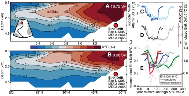
Fig. 1. Core locations. IODP Site U1305 (57°29’N, 48°32’W; 3459 m), MD03-2664

345

(57°26′N, 48°36′W; 3442 m), MD03-2665 (57°26’N, 48°36’W; 3440 m), and IODP Site

346

U1304 (53°03′N, 33°32′W; 3082 m) projected on a western Atlantic north-south section of

347

preindustrial δ13C (δ13CPI) (22) plotted using Ocean Data View. Core sites depicted in the data

348

composites of Fig. 3C are included (light and dark purple circles). Inset, plotted using

349

GeoMapApp, shows the key subpolar core sites including MD99-2227 (58°21’N, 48°37’W;

350

3460 m) and the main spreading pathways of Nordic Seas-sourced deep water contributing to

351

lower NADW (red).

352 353 354

17

355

Fig. 2. IODP Site U1305 MIS 7e, 9e, and 11c C. wuellerstorfi stable isotope and ice-rafting

356

records. A) Benthic δ18O from IODP Site U1305 (thin blue line, sample average of replicate

357

measurements; bold dark blue, 3-point running mean; shading, the standard error of the 3-point

358

window), age model tuning target ODP Site 983 (60°23’N, 23°38’W; 1983 m) (black; dashed

359

lines denote prolonged gaps) (33), and LR04 for reference (gray) (34); B) Site U1305 C.

360

wuellerstorfi δ13C (black, sample average; red, 3-point running mean; shading, standard error

361

of 3-point window) with dashed vertical lines denoting approximate levels of NADW

362

influence; C) position of age model tie points (triangles) and Site U1305 ice-rafted debris

363

(IRD; % of >150 µm entities; black and gray) (19). All records are on the LR04 timescale (19).

364

The sample spacing gives the benthic stable isotope records a nominal time resolution of 70

365

years during the interglacial benthic δ18O plateaus (shaded yellow). Insets show examples of

366

the C. wuellerstorfi δ13C variability (coloring as in B, individual data as dots). VPDB, Vienna

367

Pee Dee Belemnite standard.

368 369

18

370

Fig. 3. Variability in NADW ventilation during interglacials MIS 1-11c. Focused on the

371

interglacial δ18_{O plateaus: A) 65°N insolation at June 21}st _{(orange) (35); B) core MD99-2227}

372

records of GrIS sediment discharge showing silt sourced from Precambrian Greenland terranes

373

(green, % of total silt) (32) and from different Greenland provenances (% of sediment: colored,

374

see text inset) (18, 32, 36); C) bottom water δ13C reconstructions from mid-depth North (light

375

purple) (23) and deep South Atlantic composites (dark purple) (37) (see Fig. 1 for locations),

376

and from the deep Eirik Drift (MIS 1: 12; MIS 5e: 10; MIS 7e, 9e, and 11c: this study)

377

(coloring as in Fig. 2) with arrows denoting freshwater outburst floods as determined in (10,

378

12); and D) Eirik Drift ice-rafted debris (IRD) records (MIS 5e: 10; MIS 7e, 9e, and 11c: 19).

379

Glacial-interglacial records of: E) C. wuellerstorfi δ13C from the Eirik Drift (as in C; gray line,

380

sample average; red line, 3-point mean) and IODP Site U1304 (black and yellow, sample

381

average) (15, 38) (note difference in resolution, U1305: ~70 years; U1304: ~300 years); F)

382

Benthic foraminifera δ18O from the Eirik Drift and Site U1304 (colored, see inset; references as

383

for δ13C), and LR04 (gray) (34). All records are plotted on the LR04 timescale (19).

19

385

Fig. 4. Modeled and reconstructed deep Atlantic δ13C changes. (Left) The iLOVECLIM

386

simulated δ13_{C distribution and Eirik Drift core location (red circle) along a north-south}

387

transect (inset) averaged for years with: A) strong, modern-like AMOC (>2σ; 16.75±0.70 Sv

388

mean; n=460 model years) and NADW distribution; and B) weaker AMOC (<2σ; 8.00±0.42

389

Sv mean; n=63 model years) and shoaled NADW (see (19) for details). (Right) Across two

390

simulated NADW shoaling events (ten-year mean values): C) subpolar North Atlantic mean

391

sea surface temperature (SST; light and dark blue); D) AMOC stream function at 27°N (light

392

and dark gray); and E) Eirik Drift bottom water δ13C changes (light and dark gray; magnitude

393

similar for different preformed δ13C values, see (19)) compared to the reconstructions by

394

aligning at the last high δ13C values. To illustrate common features that account for interglacial

395

differences in preformed δ13C values, the reconstructed events are shown as the average (bold

396

lines) of multiple events (thin lines) at 30-year steps (obtained by linear interpolation) binned

397

according to durations of ≤100 (red; n=5), 101-200 (blue; n=4), and 201-300 years (green;

398

n=3).

399

20

401 402 403

Supplementary Materials for

404 405

Interglacial instability of North Atlantic Deep Water ventilation

406 407

Eirik Vinje Galaasen, Ulysses S. Ninnemann, Augustin Kessler, Nil Irvalı, Yair Rosenthal,

408

Jerry Tjiputra, Nathaëlle Bouttes, Didier M. Roche, Helga (Kikki) F. Kleiven, David A.

409

Hodell.

410 411

Correspondence to: [email protected]

412 413 414

This PDF file includes:

415 416

Materials and Methods

417 Supplementary Text 418 Figs. S1 to S7 419 References 39-57 420 421

Other Supplementary Materials for this manuscript include the following:

422 423 Data S1 [Eirik-Drift_MIS-7e-9e-11c.xlxs] 424 425 426 427 428 429 430

21 Materials and Methods

431

Sample processing and C. wuellerstorfi stable isotopes

432

The International Ocean Drilling Program (IODP) Site U1305 intervals spanning

433

Marine Isotope Stage (MIS) 7e, 9e, and 11c were identified from the stable isotope stratigraphy

434

of Hillaire-Marcel et al. (39) and continuously subsampled at 2-cm spacing at the IODP

435

Bremen Core Repository by the curatorial staff. Bulk sediment samples were kept in deionized

436

water on a shaker for 12 hours for disaggregation before being wet sieved using a 63 µm mesh

437

sieve to separate the fine (<63 µm) and coarse fraction material (>63 µm). Following wet

438

sieving, samples were dried at 50°C.

439

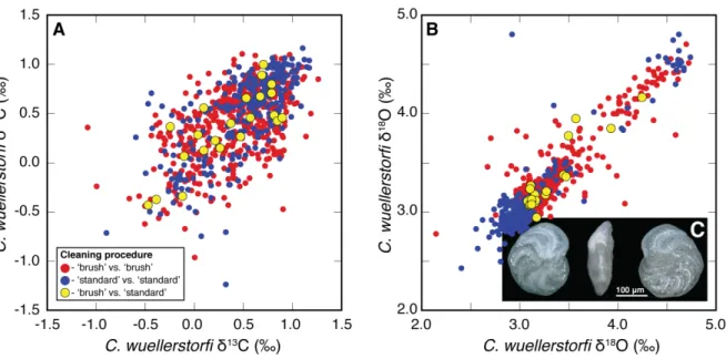
Epibenthic foraminifera Cibicidoides wuellerstorfi (sensu stricto) shells (Fig. S1) were

440

selectively picked from the >150 µm sediment fraction for stable isotope analyses. The stable

441

isotope analyses were performed at the Facility for advanced isotopic research and monitoring

442

of weather, climate and biogeochemical cycling (FARLAB), Department of Earth Science,

443

University of Bergen, Norway, on a Finnigan MAT 253 mass spectrometer coupled to an

444

automated Kiel IV preparation line kept at constant 70°C. Measurements were performed on

445

one to three individual C. wuellerstorfi shells, depending on availability and size, and

446

duplicated per sample when possible (~64% of the samples analyzed). Fig. S2 shows the C.

447

wuellerstorfi stable isotope results from Site U1305 including all individual data points. We

448

used Carrera Marble (CM12) as a working standard measured parallel to the foraminifera

449

samples, and all values are reported relative Vienna Pee Dee Belemnite (VPDB) calibrated

450

using National Bureau of Standards (NBS) standard NBS 19 and NBS 18. The long-term

451

reproducibility (1σ) of in-house standards over the analysis period was ≤0.08‰ and ≤0.04‰

452

for δ18O and δ13C, respectively. The standard cleaning step for foraminiferal stable isotope

453

analyses, involving methanol and ultrasonication, was avoided to retain mass and increase the

454

number of measurements possible, as C. wuellerstorfi shells were generally few and small in

455

size, often providing a total weight at the lower limit possible for analysis (~10-15 µg). Instead

456

of performing the standard cleaning step, C. wuellerstorfi tests were visually cleaned using a

457

brush and deionized water (‘brush-cleaned’) to remove any foreign material on or within them

458

prior to stable isotope analyses. To test the impact of omitting the standard cleaning step, we

459

measured surplus shells from samples (n=22) containing sufficient mass that were cleaned

460

following standard protocols (‘standard-cleaned’) for removing fine-grained material: adding

461

methanol to reaction vials containing the shells and keeping them in an ultrasonic bath for 10

462

seconds before extracting the methanol. The δ18O and δ13C values of the ‘standard-cleaned’ C.

463

wuellerstorfi tests are very similar to the sample average of the ‘brush-cleaned’ tests (Fig. S1).

464

Further, the intra-sample reproducibility of the ‘brush-cleaned’ Site U1305 C. wuellerstorfi

465

δ18O and δ13C data is similar to a large data set of exclusively ‘standard-cleaned’ C.

466

wuellerstorfi shells from the same region (the MIS 5e section of MD03-2664; location shown

467

in Fig. 1) (Fig. S1). This indicates that the visual ‘brush-cleaning’ and ‘standard-cleaning’ steps

468

performed similarly well with no discernible difference in the stable isotope values or in the

469

intra-sample variability. Nonetheless, performing the standard cleaning step for foraminiferal

470

stable isotope analyses is highly recommended when possible. Indeed, in certain regions and

471

time intervals, a cleaning procedure more stringent than the standard one is likely required to

472

accurately determine foraminiferal stable isotope values (40).

473 474

C. wuellerstorfi B/Ca

22

We measured B/Ca ratios in C. wuellerstorfi tests from intervals in MD03-2664 (MIS

476

5e) and Site U1305 (MIS 7e, 9e, and 11c). To obtain sufficient mass for B/Ca analyses

(~250-477

300 µg), and due to scarcity of C. wuellerstorfi tests in these sediments, it was often necessary

478

to combine tests from up to a maximum of six adjacent samples (or 12 cm of core) that we

479

restricted according to consistent C. wuellerstorfi δ13C values. Following the selective picking,

480

the C. wuellerstorfi tests were opened using clean glass slides and transferred into acid-leached

481

vials. The C. wuellerstorfi tests were subsequently cleaned for contaminating phases, including

482

clay removal, reductive and oxidative steps, a weak acid leach, and dissolution in dilute HNO3.

483

The B/Ca analyses were performed using the method outlined in Rosenthal et al. (41) on a

484

Finnigan MAT Element XR Sector Field Inductively Coupled Plasma Mass Spectrometer

485

(ICP-MS) at the ICP-MS laboratory at the Institute of Marine and Coastal Sciences, Rutgers,

486

The State University of New Jersey, USA.

487 488

Site U1305 N. pachyderma (s) δ13_{C records}

489

N. pachyderma (s) tests were selectively picked from the 150-212 µm sediment fraction

490

at continuous 4-cm spacing across MIS 7e, 9e, and 11c (with notable gaps only in MIS 9e due

491

to scarcity of N. pachyderma (s) tests). Prior to the stable isotope analyses, the tests were

492

cleaned by adding methanol to the sample kept in reaction vials and ultrasonicating them for

493

ten seconds before removing the supernatant. The stable isotope analyses were performed at

494

FARLAB, University of Bergen, Norway, as outlined for benthic foraminifera C. wuellerstorfi

495

above, and with identical standard reproducibility. Measurements on N. pachyderma (s) were

496

replicated whenever possible (~92% of the samples), and each individual measurement was

497

performed on 6-10 individual N. pachyderma (s) tests.

498 499

Ice-rafted debris

500

The ice-rafted debris (IRD) counts were performed on the same Site U1305 samples as

501

the benthic foraminiferal stable isotope measurements, but at lower sampling density. IRD

502

counts were performed at 32-cm spacing for MIS 7e and 11c, and 16-cm spacing for MIS 9e

503

(42). Following the sample processing steps outlined above, material in the >150 µm fraction

504

were split, IRD grains visually identified, and IRD calculated as the percent of ≥300 counted

505

entities.

506 507

Hole U1305C MIS 11c mcd fine-tuning

508

Sediment physical properties (e.g., magnetic susceptibility) indicated cm-scale offsets

509

between Hole U1305C and the original (Hole A & B) splice over ~74.5-78.5 mcd (Fig. S3A),

510

corresponding to most of MIS 11c. We fine-tuned the mcd scale for the Hole U1305C MIS 11c

511

interval using magnetic susceptibility, shifting it between -3 cm and -19 cm to align the

512

physical property records (Fig. S3B), and include both the original and corrected core depth

513

scales in the MIS 11c data table.

514 515

iLOVECLIM model simulation

516

We used the iLOVECLIM Earth system model of intermediate complexity to simulate

517

and assess potential relationships between NADW distribution, northwest Atlantic bottom

518

water δ13_{C, and AMOC. The iLOVECLIM model is an isotope-enabled development branch of}

519

LOVECLIM version 1.2 (43) and includes an ocean component (CLIO) with 20 vertical layers

520

and 3° by 3° horizontal resolution as well as land and ocean carbon cycle modules (25). We

23

performed a transient simulation for 125-115 ky (corresponding to MIS 5e) using annually

522

interpolated greenhouse gas and orbital forcings following the third phase of the Paleoclimate

523

Modelling Intercomparison Project (PMIP; https://pmip3.lsce.ipsl.fr/), initialized from a

quasi-524

equilibrium spin up of 5000 years forced with constant 125 ky boundary conditions. We

525

performed two quasi-equilibrium spin-ups prior to the 125-115 ky simulation, each integrated

526

for 5000 years. The first is based on preindustrial conditions and the second on 125 ky

527

boundary conditions. The preindustrial simulation was used to validate and confirm that

528

iLOVECLIM reproduces the spatial distribution of preindustrial ocean δ13C (22), and the 125

529

ky spin-up to initialize the 125-115 transient simulation. To test the sensitivity of the simulated

530

deep Atlantic δ13C variability to changes in surface biological processes and preformed δ13C

531

values, we ran to additional 125-115 ky transient simulations using similar initial conditions as

532

above but starting at 125 ky with either: 1) atmospheric δ13C fixed at value decreased by

533

~0.6‰ (at -7.1‰); or 2) with 50% decreased primary productivity in the modeled convection

534

regions off southern Greenland and in the Nordic Seas. We expand on the model results in the

535

discussion section of the supplement below.

536

The modeled inorganic carbon cycle is represented by dissolved inorganic carbon

537

(DIC) and alkalinity (ALK), while the organic carbon cycle includes phytoplankton,

538

zooplankton, dissolved organic carbon (DOC), slow dissolved organic carbon (DOCs),

539

particulate organic carbon (POC), and CaCO3. The phytoplankton is partially remineralized as

540

it sinks through the water column, while all the POC and CaCO3 is remineralized at depth. The

541

remineralization profile follows an exponential law, adjusted to have less remineralization in

542

the upper layers and more at depth. Carbon fractionation during photosynthesis fixes 12C in the

543

organic matter, which is added back by the remineralization process at depth. At the air-sea

544

interface, the carbon flux is computed from the CO2 partial pressure difference between the

545

atmosphere and ocean at a constant gas exchange coefficient of 0.06 mol m-2 yr-1, where sea

546

surface pCO2 is a function of temperature, salinity, DIC, and ALK following Millero (44). The

547

modeled δ13C distribution is thus affected by air-sea gas exchange and organic matter

548

production/remineralization, and transported by the advection-diffusion scheme of the model.

549

Unlike 12C, the atmospheric 13C is prognostically simulated in response to land and ocean

550 processes. 551 552 Supplementary Text 553

Site U1305 age model

554

The age models for the MIS 7e, 9e, and 11c intervals of Site U1305 were constructed

555

by correlating our benthic δ18O record to and adopting the age model constructed for ODP Site

556

983 (33, 45) (Fig. 2, Fig. S4). Using Site 983 benthic δ18O as a tuning target has advantages

557

over other reference records. First, Site U1305 shares well-defined structures in benthic δ18O

558

with Site 983 (Fig. 2; Fig. S4) allowing relatively robust correlation. Further, high-resolution

559

IRD records are available from both sites and allow us to validate the benthic δ18O-correlation

560

near deglacial intervals where Site U1305 benthic δ18O data were often lacking due to C.

561

wuellerstorfi absence (Fig. 2). Tie points were defined based on major benthic δ18O transitions

562

and linearly interpolated between to obtain ages for all core depths (Fig. S4). The Site U1305

563

and MD03-2664 IRD records were also used to guide the determination of tie points at the start

564

of the interglacial δ18_{O plateaus, as deglacial IRD increases are observed to coincide with}

565

transient decreases in benthic δ18O values before MIS 5e (10) and MIS 7e, 9e, and 11c in this

24

region (Fig. 2; Fig. S4). Given their transient nature and co-occurrence with deglacial IRD,

567

these deglacial benthic δ18O reductions may reflect contamination from low-δ18O detrital

568

carbonate commonly deposited during Heinrich-events (40). Consequently, deglacial samples

569

with low C. wuellerstorfi δ18_{O and high IRD were disregarded when we constructed our age}

570

model and we defined the first interglacial benthic δ18O value, and start of the interglacial

571

plateaus, as the first continuously low δ18O value occurring after large deglacial IRD increases.

572

Corroborating this approach, the Site U1305/MD03-2664 and Site 983 deglacial IRD peaks

573

align using this additional constraint for the benthic δ18O tuning (Fig. S4) but would otherwise

574

be offset by a few thousand years.

575

Age uncertainties involved with benthic δ18O-based age models can be considerable.

576

For example, age differences between major δ18O transitions can reach up to a few thousand

577

years between different ocean basins (46). The absolute age uncertainty provided by the Site

578

U1305-Site 983 correlation is likely less than millennial, given i) the relative proximity of

579

these core sites, ii) the similarity of the benthic δ18_{O records—indicating a shared δ}18_O

580

evolution, and iii) the alignment of deglacial IRD peaks (Fig. 2; Fig. S4). Despite a relatively

581

robust correlation, the original age model still carries considerable uncertainty in absolute ages.

582

For example, adopting a different age model constructed for Site 983 by Barker et al. (45) (e.g.,

583

EDC3 and AICC2012), would shift absolute ages up to a few thousand years.

584

In addition to absolute age uncertainties, relative (sample-to-sample) age uncertainties

585

likely also exist for the Eirik Drift (Site U1305 and MD03-2664) records. Correlation of

586

benthic δ18O records is achieved using a limited number of tie points. This is especially true for

587

interglacial δ18O plateaus, here defined by two (MIS 5e, 7e, and 9e) or three (MIS 11c) tie

588

points (Fig. 2, Fig. S4). These tie points were linearly interpolated between, assuming constant

589

sedimentation rates. However, interglacial sedimentation rates can vary on a range of

590

timescales in this area (39, 47-49). For example, radiocarbon-dated sections indicate that

591

sedimentation rates were higher in the early compared to the late phase of the current

592

interglacial at multiple Eirik Drift locations (e.g., 12, 48). If this temporal sedimentation pattern

593

persisted in the older interglacial periods, our age models based on the conservative approach

594

of linear interpolation may over- and underestimate the durations of early and late interglacial

595

intervals, respectively.

596 597

Site U1304, MD03-2664, MD03-2665, and MD99-2227 age models

598

To place all proxy records on a common age scale, we revised the age models for all

599

core intervals containing data we compare to the IODP Site U1305 records. We tuned the MIS

600

5e interval of MD03-2664 and the MIS 5e, 7e, 9e, and 11c intervals of IODP Site U1304 to the

601

same ODP Site 983 reference record (Fig. S4), applying identical tie points and linearly

602

interpolating between as outlined above. The MIS 1 and last deglacial intervals of Site U1304

603

and MD03-2665 were left on their original age models as presented in Xuan et al. (38) and

604

Kleiven et al. (12), respectively.

605

To compare our records to the MD99-2227 southern Greenland sediment discharge

606

reconstructions (18, 32, 36), we transferred our benthic δ18O-based age models for MIS 5e

607

(MD03-2664), 7e, 9e, and 11c (Site U1305) to MD99-2227 by correlating magnetic

608

susceptibility between this core and MD03-2664 (MIS 5e) and Site U1305 (MIS 7e, 9e, and

609

11c) (Fig. S5). The strong similarity of the magnetic susceptibility records indicate that these

610

core sites shared sedimentation histories, providing robust relative age control to comparisons

611

of the Site U1305/MD03-2664 and MD99-2227 records. The alignment of glacial and

25

interglacials values in epibenthic foraminifera C. wuellerstorfi δ18O from MD03-2664/Site

613

U1305 and planktic foraminifera N. pachyderma (s) δ18O from MD99-2227 on the obtained

614

age models supports the magnetic susceptibility correlation (Fig. S5). Carlson et al.’s (50) age

615

model was used for the MIS 1 and last deglacial intervals of MD99-2227.

616 617

C. wuellerstorfi B/Ca and N. pachyderma (s) δ13C

618

To test the fidelity of Eirik Drift C. wuellerstorfi δ13C as recorder of bottom water

619

carbon chemistry and water mass tracer, we use epibenthic foraminifera C. wuellerstorfi B/Ca,

620

a proxy for bottom water carbonate ion saturation (Δ[CO32-]) and independent metric of the

621

influence of high-[CO32-] NADW versus low-[CO32-] SSW (e.g., 51, 52). The Eirik Drift C.

622

wuellerstorfi B/Ca data span a range of 185-215 µmol/mol with distinct changes within each of

623

MIS 5e, 7e, 9e, and 11c (Fig. S6). Using Yu & Elderfield’s (51) B/Ca to Δ[CO32-] relationship

624

for C. wuellerstorfi, the B/Ca data indicates intra-interglacial changes in bottom water [CO32-]

625

by 25-30 µmol/kg, similar to that expected from shifting between NADW and SSW influence

626

(e.g., 52). The concurrent and coupled changes in C. wuellerstorfi δ13C by up to ~0.8‰ within

627

the same sample pool (Fig. S6) is similarly consistent with shifts between NADW and SSW

628

influence. Indeed, the paired change in Eirik Drift C. wuellerstorfi B/Ca and δ13C we observe is

629

similar to that recorded in the last glacial to Holocene sections of two North Atlantic cores

630

from similar water depths (Fig. S6) that was previously interpreted to reflect the

well-631

established deglacial shift from SSW to NADW influence in the deep North Atlantic (52). We

632

suggest that the Eirik Drift C. wuellerstorfi B/Ca record supports the interpretation of the C.

633

wuellerstorfi δ13C variability as reflecting changes in NADW versus SSW influence.

634

An alternative explanation for co-variability in trace element ratios and δ13C is

635

contamination by secondary CaCO3 precipitation and presence of authigenic overgrowths.

636

However, several lines of evidence argue against a role for contamination by secondary CaCO3

637

precipitation. The C. wuellerstorfi δ13C record suggest no discernible influence by its own

638

merit, showing for example i) absolute values within the range of values observed in the

639

modern ocean or relevant reconstructions (e.g., 22, 23; Fig. 3) and ii) a consistency in the

640

signal and a lack of extremely large fluctuations that would require the mass and isotope value

641

of any contamination to have adjusted itself to balance changes in the mass and isotope value

642

of the foraminifera tests. Further, secondary CaCO3 precipitation should, if present, influence

643

all foraminifera tests in a given core depth to some degree similarly. That is, if secondary

644

CaCO3 precipitation drove relatively large changes in C. wuellerstorfi δ13C and B/Ca, planktic

645

foraminifera δ13_{C should also show low δ}13_{C values in addition to some degree of}

co-646

variability. The Eirik Drift N. pachyderma (s) δ13C records from MIS 5e, 7e, 9e, and 11c do not

647

show values as low as the C. wuellerstorfi δ13C records and there is no significant relationship

648

between N. pachyderma (s) and C. wuellerstorfi δ13C (Fig. S6). In sum, we suggest secondary

649

CaCO3 precipitation is either unimportant or entirely absent and consider it as an unlikely

650

explanation for the co-variability in C. wuellerstorfi B/Ca and δ13C. Changes in the influence

651

of NADW versus SSW could conversely explain these observations.

652 653

iLOVECLIM model simulation results

654

We identified persistent centennial-scale variability in δ13C and the distribution of

655

NADW in our 125-115 ky transient simulation occurring over a ~6 ky long interval in-between

656

intervals of relative stability during the initial 2-3 and final 1-2 ky. A subsequent study will

657

outline and discuss the results of the model simulation in detail (Kessler et al., in prep.). Here,

26

we use the simulation to help the interpretation of the reconstructed bottom water δ13C

659

variability by assessing how centennial-scale changes in NADW distribution can impact deep

660

Atlantic δ13C. We focus on the simulated episodes of NADW shoaling and recovery to assess

661

the possible rate, duration, and magnitude of water mass distribution and associated bottom

662

water δ13C changes and compare these to the reconstructed δ13C variability. In the simulation,

663

episodes of NADW shoaling were abruptly initiated, lasted some centuries, and were

664

associated with decreases in AMOC strength and North Atlantic bottom water δ13C (Fig. 4).

665

The simulated episodes of NADW shoaling/deepening produced distinct North Atlantic

666

bottom water δ13C variability as (low-δ13C) Southern source water (SSW) expanded/contracted

667

in concert with (high-δ13C) NADW contracting/expanding (Fig. 4). In the northwest Atlantic

668

region corresponding to the location of Eirik Drift core sites U1305, 2664, and

MD03-669

2665, shoaling of NADW and incursions of SSW manifested as ~0.4‰ decreases in bottom

670

water δ13C achieved over a few decades, events that ended equally abrupt as NADW deepened

671

some centuries (~100-500 years) later (Fig. 4). To illustrate these NADW and δ13_{C distribution}

672

changes, Fig. 4A and Fig. 4B displays the North Atlantic mean δ13C distribution below 500 m

673

water depth for all simulated years with anomalously strong AMOC (>2σ; n=460 model years;

674

mean AMOC strength: 16.75±0.70 Sv) and anomalously weak AMOC (<2σ; n=63 model

675

years; mean AMOC strength: 8.00±0.42 Sv), respectively. We further selected two simulated

676

intervals of NADW shoaling and recovering to compare to the reconstructed bottom water δ13C

677

variability (Fig. 4B), differing from other simulated shoaling episodes only in duration. The

678

magnitude of any bottom water δ13C variability driven by such changes in the relative

679

influence of northern versus southern source water could depend strongly on the preformed

680

δ13C of, and the gradient between, competing water masses. While iLOVECLIM captures the

681

preindustrial preformed δ13_{C of northern and southern source waters relatively well (e.g.,}

682

compare Fig. 1 to Fig. 4A), proxy records suggest considerable changes in preformed water

683

mass δ13C occurred between and even within past interglacial periods. For example, the

684

preformed δ13C of northern source water may have been higher in the Holocene than the late

685

Pleistocene interglacials (see data composites, purple lines, in Fig. 3), while it likely increased

686

across MIS 5e (Fig. 3) consistent with planktic and epibenthic foraminifera δ13C records from

687

the Nordic Seas (e.g., 53). This model-data difference should be noted when comparing and

688

contrasting the simulated and reconstructed time series. For the proxy reconstructions, we took

689

this into account by averaging multiple events in order to illustrate common features

690

independent of specific interglacials and preformed δ13C values (Fig. 4). Still, the similarity of

691

the modeled and reconstructed bottom water δ13_{C changes could result from the simulation}

692

having a specific set of preformed δ13C values in NADW and SSW. To assess how different

693

background states and preformed δ13C in NADW and SSW could impact the magnitude and

694

character of the simulated bottom water δ13C variability, we reran the simulation twice with 1)

695

atmospheric δ13C lowered by ~0.6‰ and 2) 50% decreased primary productivity in the

696

simulated deep water formation regions off southern Greenland and in the Nordic Seas. Both

697

experiments shift the absolute values of the simulated Eirik Drift bottom water δ13C time series

698

but in both cases the relative magnitudes and character of the variability is only negligibly

699

impacted (Fig. S7). The simulation with perturbed primary productivity, resulting in limited

700

change in deep Atlantic δ13C, supports previous studies suggesting that organic carbon fluxes

701

have little influence on the δ13_{C of C. wuellerstorfi (e.g., 21). Thus, the character of the Eirik}

702

Drift bottom water δ13C variability driven by shifts in the distribution of water masses appears

703

to be relatively stable in face of different preformed δ13C values and background biological