Shape from sensors: Curve networks on surfaces from 3D orientations

HAL Id: hal-01524740

https://hal.inria.fr/hal-01524740v2

Submitted on 19 May 2017

HAL is a multi-disciplinary open access

archive for the deposit and dissemination of

sci-entific research documents, whether they are

pub-lished or not. The documents may come from

teaching and research institutions in France or

abroad, or from public or private research centers.

L’archive ouverte pluridisciplinaire HAL, est

destinée au dépôt et à la diffusion de documents

scientifiques de niveau recherche, publiés ou non,

émanant des établissements d’enseignement et de

recherche français ou étrangers, des laboratoires

publics ou privés.

Shape from sensors: Curve networks on surfaces from

3D orientations

Tibor Stanko, Stefanie Hahmann, Georges-Pierre Bonneau, Nathalie

Saguin-Sprynski

To cite this version:

Tibor Stanko, Stefanie Hahmann, Georges-Pierre Bonneau, Nathalie Saguin-Sprynski. Shape from

sensors: Curve networks on surfaces from 3D orientations. Computers and Graphics, Elsevier, 2017,

Special Issue on SMI 2017, 66, pp.74-84. �10.1016/j.cag.2017.05.013�. �hal-01524740v2�

Shape from sensors: curve networks on surfaces from 3D orientations

Tibor Stankoa,b_{, Stefanie Hahmann}b_{, Georges-Pierre Bonneau}b_{, Nathalie Saguin-Sprynski}a a_{CEA, LETI, MINATEC Campus, Université Grenoble Alpes}

b_{Université Grenoble Alpes, CNRS (Laboratoire Jean Kuntzmann), INRIA}

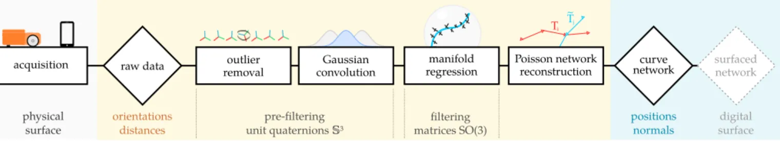
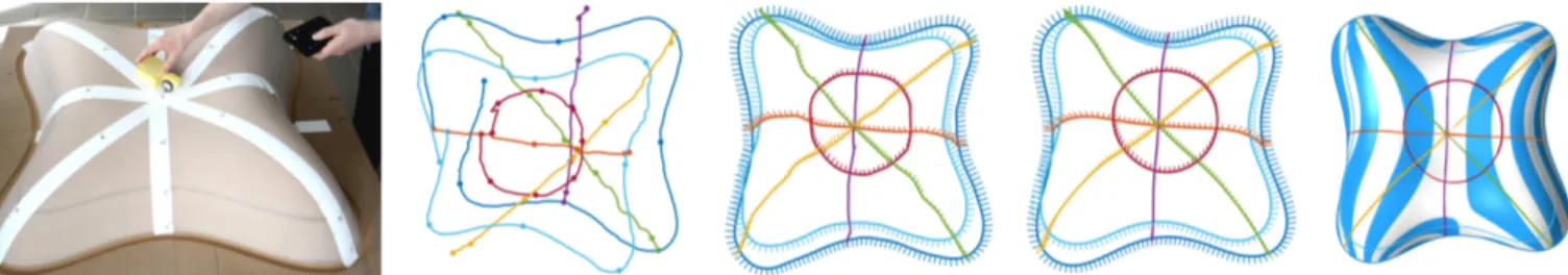
Figure 1: Surface of the lilium is scanned by acquiring orientations along curves using a sensor-instrumented device (left). Naive integration of the scanned data fails to close the network (middle left). Reconstructing the network by solving a Poisson system resolves topological problems but yields noisy and inconsistent normals (middle). Filtering orientations prior to Poisson reconstruction gives a consistent network (middle right) available for surface fitting (right). See the accompanying video for the acquisition setup.

Abstract

We present a novel framework for acquisition and reconstruction of 3D curves using orientations provided by iner-tial sensors. While the idea of sensor shape reconstruction is not new, we present the first method for creating well-connected networks with cell complex topology using only orientation and distance measurements and a set of user-defined constraints. By working directly with orientations, our method robustly resolves problems arising from data inconsistency and sensor noise. Although originally designed for reconstruction of physical shapes, the framework can be used for “sketching” new shapes directly in 3D space. We test the performance of the method using two types of acquisition devices: a standard smartphone, and a custom-made device.

Keywords: curve networks, shape acquisition, surface reconstruction, inertial sensors, 3D sketching

1. Introduction

Curve networks play an important role in CAD and of-ten serve for conveying designs [Coons,1967;Moreton & Séquin,1991]. At the same time, well-defined curve net-works are used for automatic inference of underlying sur-faces by minimizing fairing energy or using methods with prescribed degree of continuity.

Recent research in sketch-based modeling and virtual reality produced tools and devices for intuitive design of 3D curves (Fig. 3). These tools and devices attempt to overcome some of the limitations of the traditional CAD approach – designers can sketch curves directly, either on a flat screen or via a 3D interface. Although intuitive, these methods are targeted towards design of new shapes and are not suitable for reconstruction of existing real-world shapes.

We present a novel framework for acquisition of 3D curves using orientations measured by inertial sensors. While the idea of sensor shape reconstruction is not new, we present the first method for creating well-connected networks of curves on surfaces using only orientation and distance measurements and a small set of user-defined

constraints. We address three main challenges that arise when working with sensor data.

• Unknown positions. Sensors measure local orien-tations of the surface – no absolute positions in the world space nor relative positions of two adjacent sensors are known.

• Inconsistent data. Intersecting curves often provide conflicting data, for instance two different normals for the same point in the world space.

• Sensor noise. Raw data from inertial sensors is noisy and needs to be pre-processed prior to recon-struction.

Our approach differs from standard curve acquisition and reconstruction methods in the fact that we formulate all algorithms in terms of orientations. This way, we can leverage consistency of reconstructed curves with respect to user-defined topological constraints. By working di-rectly with orientations, our framework robustly resolves all above challenges in two steps. We first filter the acqui-sition noise by combining pre-filtering of the raw

orienta-tions in the quaternion space with a spline-based smooth-ing in the group of rotations (Sec.4). We then introduce a curve-based Poisson reconstruction method, which trans-forms the pre-filtered orientation samples into a smooth and consistent curve network by satisfying in particular the user annotated topological constraints (Sec.5). To en-able a thorough evaluation and comparison with respect to ground truth data (Sec.6), we use two physical objects fabricated from digital models: the lilium (Fig.1) and the cone (Fig.15).

To demonstrate our framework, we use a dynamic

ac-quisition setup, where we suppose the data is measured by

a single moving node of sensors. We test and compare two types of devices: a standard smartphone, and a custom-made prototype for measuring orientations and distances (Fig. 10). Nevertheless, the algorithms presented in this paper are not limited to these devices; they are also ap-plicable in a static acquisition setup, such as a grid/mesh of sensors [Saguin-Sprynski et al.,2014;Sprynski,2007] or instrumented materials [Hermanis et al.,2016].

The primary application of the presented framework is reconstruction of existing shapes. Our setup provides a valuable alternative to traditional shape acquisition meth-ods (3D scanners, depth images). Unlike most 3D scan-ners, which often use cameras and lasers, inertial sensors are independent from light conditions, material’s optical properties and scale of the scanned object. They render the acquisition possible outdoors or underground, and can also be used for large and/or moving objects; imag-ine acquisition of underground pipes [Saguin-Sprynski et al.,2016], or an instrumented sail moving in the wind (Fig. 20). Possible applications include smart materials and structural health monitoring.

A major advantage of our approach is its generality. No special device is required for data acquisition; in fact, any sensor-instrumented device could be used for the task, thus making 3D acquisition accessible to everyone with an ordinary smartphone. Even though originally designed for reconstruction, our framework can also be used for design by “sketching” new shapes from scratch (Fig.2).

Figure 2: The mushroom network created from scratch entirely with a smartphone. Curve lengths were estimated from acquisition time. The surfacing was computed using the method ofStanko et al.[2016] with soft positional constraints.

Figure 3: Recent curve acquisition devices that use inertial sensors. Left to right: Tilt Brush [Google], SmartPen [Milosevic et al.,2016] and 01 [InstruMMents,2017].

2. Related work

Shape from curves. The problem of generating shapes from collections of curves has been well studied in CAGD (Computer Aided Geometric Design) and all standard techniques can be found in Farin [2002]. In the recent years, the interest in this problem was re-ignited due to its applications in sketch-based modeling [Andrews et al.,

2011;Bae et al.,2008;Igarashi et al.,1999;Nealen et al.,

2007;Xu et al.,2014] and in virtual reality (VR) systems [Google]. Inspired by years of research in CAGD, the

sur-face from curves paradigm is invaluable for shape design in

modern sketching and VR systems. Recently,Arora et al.

[2017] have studied issues with accurate design of shapes in the existing VR systems. Their study suggests that users struggle even with simple tasks (drawing a closed circle) when sketching in three dimensions. A system like ours can help in solving such accuracy and consistency is-sues.

Although equally important, the problem of

recon-struction of existing physical shapes from a collection of

curves received less attention. 3D scanners usually pro-vide large amounts of data and tend to ignore intrinsic structure of the scanned shape. Alternatively, objects can be defined by their characteristic curves as often done in perception and sketch-based modeling. Cao et al.[2016] detect characteristic curves in noisy point clouds, then use these curves for surface reconstruction. The use of inertial measurement units (IMUs) for shape acquisition might provide a good alternative in situations for which the opti-cal methods do not yield proper results, positioning sen-sors along object’s characteristic curves. Milosevic et al.

[2016] introduced SmartPen, a low-cost system for captur-ing 3D curves, which combines an IMU with a stereo cam-era (Fig.3middle). By combining a stereo camera with a sensor unit, their system is a mixture of traditional 3D scanners and our shape from sensors setup. However, SmartPen’s sensors only serve for determining device’s orientation needed for estimating relative position of the tip of the pen. Much like traditional point-cloud scanners, the system relies on visual input to get 3D position of the device in world space; this limits size of the scanned ob-ject. A recent example of curve acquisition device is the commercially available 01 [InstruMMents,2017], a dimen-sioning tool with an IMU and a laser (Fig.3 right). Al-legedly, the device can be used to reconstruct 3D curves; this claim rests to be verified experimentally.

outlier removal

manifold regression

raw data Poisson network_{reconstruction network}curve

pre-filtering

unit quaternions 𝕊³ matrices SO(3)filtering

surfaced network acquisition physical surface orientations distances positions normals Gaussian convolution Ti Tj ~ digital surface

Figure 4: A schematic overview of our shape from sensors framework. First, the orientations and distances acquired from the physical surface are pre-filtered (Sec.4.2) using efficient averaging schemes in the quaternion space (Sec.4.1). Second, the pre-filtered data are smoothed using regression on the manifold of orientation matrices (Sec.4.3) to obtain smoothly varying frames with consistent normals. Finally, the positions are reconstructed by solving a sparse linear Poisson system for the whole network (Sec.5).

Shape from sensors. The use of sensors for shape acquisition was first explored by Sprynski [2007]. In-stead of measuring absolute position of surface points of the scanned object in the world space, the reconstruc-tion algorithms need to be formulated in terms of orien-tations provided by sensors, and geodesic distances be-tween points of measurement. Curves are represented using natural parametrization and reconstructed via nu-merical integration. Surfaces are defined via geodesic in-terpolation [Sprynski et al.,2008] or using parallel rib-bons of sensors [Saguin-Sprynski et al.,2014].Huard et al.

[2013] introduced method for computing smooth patches from a given piecewise geodesic boundary curve. Hoshi & Shinoda[2008] reconstruct the target surface using two families of sensors placed in orthogonal directions. Her-manis et al. [2016] construct sensor-instrumented fabric and compare the reconstruction results with Kinect data.

Antonya et al.[2016] use an array of sensors for real-time tracking of human spine.

Attitude estimation and filtering. Attitude control has been studied extensively in aeronautics where accu-rate algorithms are indispensable for correct estimation of vehicle’s orientation with respect to celestial objects [Markley & Mortari,2000]. Noise in data is usually re-duced using a Kalman filter – specific approaches de-pend on the representation used for orientations [ Cras-sidis et al.,2007], such as unit quaternions, a representa-tion well-known in the graphics community [Shoemake,

1985]. Markley et al.[2007] describe a classical algorithm for computing means in the group SO(3). Average rota-tion is defined as the minimizer of weighted penalty func-tion, and the corresponding unit quaternion is computed efficiently via eigendecomposition of a 4-by-4 matrix; see Sec.4.1for more details.

Apart from statistical approaches such as Kalman fil-ters, geometric methods can be used to denoise orienta-tions.Shoemake[1985] introduced quaternion splines us-ing spherical Bézier curves;Nielson[2004] later extended this algorithm and introduced ν−quaternion splines. Al-though spline methods work well for interpolation of ro-tations in a sequence of keyframes, the Bézier representa-tion is not suitable for filtering noisy orientarepresenta-tions. Energy-minimizing splines for data in Euclidean spaces have

been well-studied. Reinsch[1967] introduced smoothing splines that minimize stretching and bending while ap-proximating given data in a Euclidean space. Hofer & Pottmann[2004] describe a method for computing such splines for data on a Riemannian manifold M. Data are first optimized in the ambient (Euclidean) space, then pro-jected onto M; these two steps are repeated until conver-gence. An equivalent result can be found by optimizing data directly on the manifold [Boumal & Absil,2011]. In this sense, classical splines are obtained for M = Ed. We

use smoothing splines on the manifold SO(3) to filter raw orientation data from sensors (Sec.4.3).

Poisson reconstruction. Poisson’s equation ∆φ = ∇ ·V often arises in the context of reconstruction of shapes (curves and surfaces).Kazhdan et al.[2006] resolve a Pois-son problem ∆χ = ∇ · N to find the indicator function φ, which implicitly defines the surface, from a sample of the surface’s oriented normal field N. This approach is a state of the art method for surface reconstruction from unor-ganized points clouds. Our reconstruction algorithm is inspired by the work ofCrane et al.[2013] who use the Poisson equation ∆ f = ∇ · T to retrieve positions f of a closed planar curve from its tangent field T during iso-metric curvature flow. We extend this approach to closed curve networks on surfaces, and use it to reconstruct po-sitions of the scanned curves (Sec.5).

Figure 5: In this example, only the top left cell complex is a valid input to our algorithm. The other three networks have non-contractible cycles (top right), violate the definition of a cell complex (bottom left) or they are disconnected (bottom right).

3. Definitions and input data

Given a smooth connected 2-manifold surface S ⊂ E3,

we consider a collection Γ of G1smooth curves embedded

on S (Γ is therefore a topological subspace of S). Curves in Γdivide the surface into a finite number of cells forming a two-dimensional cell complex C = (V, E, F ) on S, consist-ing of nodes V (0-cells), segments E (1-cells) and cycles F (2-cells) [Berberich et al.,2010;Hatcher,2002]. Moreover we suppose the cell complex is connected and the cycles are contractible (Fig.5). Each curve γ ∈ Γ can be thought of as a path in C. We say that two curves intersect at a node η ∈ Vif their corresponding paths contain η.

Denote by x : [0, L] → E3the natural parametrization

of γ ∈ Γ where L is the length of γ. For a fixed point x on the curve, the orthonormal Darboux frame D = (T, B, N) is defined as

T = x′

, N ⊥ TxS, B = N × T.

Here, TxSdenotes the two-dimensional tangent space of S at the point x ∈ S and N is chosen as the outward surface normal. We represent the Darboux frame D as an orien-tation matrix A = [T B N] ∈ SO(3), which is a member of the special orthogonal group

SO(3) = {A ∈ R3×3 _: A⊤A = I and det(A) = 1} .

We denote by A|T, A|B, A|N the projections on the first, second and third column of the matrix A, respec-tively. Throughout this paper, the terms “orientation” and “frame” refer to the same concept – the Darboux frame of a curve point with respect to the underlying sur-face.

A(x)

A|N A|T

Figure 6: For a closed network, the orientation function x 7→ A(x) is not continuous – tangent vector is different for each curve passing through an intersection. Note that the projection on the normal component A|N: Γ → S2_{(Gauss map of S restricted to curves) is closed as the surface} normal varies smoothly.

The function A : Γ → SO(3), which associates each curve point to its Darboux frame, is not continuous. In-deed, at intersections the tangent vector T differs for each adjacent curve (Fig.6). Note however that the projection on the normal component A|Nis continuous and is iden-tical to the Gauss map of S restricted to the curves in Γ.

Our goal is to retrieve the unknown positions x pro-vided a sample of orientations Ai = A (x (di))for each

curve γ at known distances di ∈ [0, L]. We suppose the

topology of the underlying cell complex C is known. The main steps of our algorithm are shown in Fig.4.

4. Filtering orientations

In this section, we describe our approach for filter-ing raw orientation data acquired usfilter-ing inertial sensors. Sensor noise and limited scanning precision are the main problems that prevent using raw orientations in the recon-struction of positions. By consequence, the acquired net-work of orientations is often inconsistent: at intersections, the normals are different for each passing curve (Fig.16). To eliminate acquisition problems, we use a two-step fil-tering process – see Fig.7. First, raw data are pre-filtered using distance-weighted Gaussian convolution with fixed edge length. This way, we obtain uniform sampling of orientations with respect to curve lengths. Second, the uniform samples are smoothed and made consistent us-ing regression on the manifold SO(3).

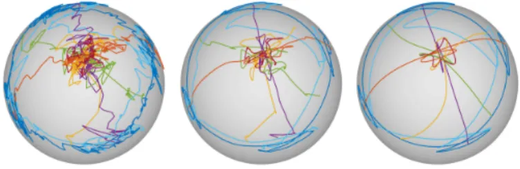
Figure 7: Two-step filtering of acquired orientations from Fig.1, here visualized using the Gauss map A|N(surface normals extracted from

orientations mapped to the unit sphere). Left to right: raw data, pre-filtered data (Sec.4.2), filtered data (Sec.4.3).

4.1. Averaging orientations

To compute (weighted) means in the group of rota-tions, it is convenient to use the quaternion representation [Markley & Mortari,2000]. The rotation around the (unit) Euler axis e by the angle 2θ is given by the unit quaternion

q = [cos θ; e sin θ] ∈ S3

⊂ H,

where S3 denotes the unit 3-sphere in the quaternion

space H ≈ R4. We will denote by A(q) the conversion

between the orientation matrix A and the unit quaternion q (seeShoemake[1985] for details).

Given a set of unit quaternions qi∈ S3with weights wi

for i = 1, . . . , N, the average quaternion ¯q is defined via the following minimization problem [Markley et al.,2007]:

¯ q = arg min q∈S3 N ∑ i=1 wi A(q) − A(qi) 2 F,

where ∥ · ∥F is the Frobenius norm. This is equivalent to

solving

¯

q = arg max q∈S3

q⊤_Mq,

where the 4x4 matrix M is the structure tensor

M =∑N

i=1

The solution to this optimization problem is known to be the (unit) eigenvector ¯q of M corresponding to the largest eigenvalue. This procedure is known as the q method. The q method is computationally efficient and naturally overcomes the fact that unit quaternions S3 are a 2-to-1

covering of the rotation group: antipodal quaternions q and −q represent the same rotation. This is why spherical linear interpolation [Slerp,Shoemake,1985] is not suitable for averaging quaternions – changing the sign of a quater-nion should not change the average, which is not the case for Slerp.

4.2. Pre-filtering via Gaussian convolution

Working with orientations which are sampled uni-formly with respect to geodesic distance facilitates both the filtering (Sec.4.3) and the reconstruction of positions (Sec. 5) – the uniform sampling is convenient for dis-cretization of differential operators and intergrals. In this section we describe the computation of such uniform sam-pling from raw orientation measures in the quaternion space.

Before computing the uniform sampling, we first re-move outliers and process duplicate measures. Outliers are removed by looking at the dot products of quaternion qiwith its immediate neighbors qi−1and qi+1. If both dot

products are smaller than the specified threshold α, the angles between qi and its neighbors are too big and qi

is removed. For the examples in this paper, we use the threshold α = 0.9; this is consistent with the assumption that the acquisition frequency is high enough and each two adjacent data points are close in the space of orienta-tions. For sparsely sampled networks, a smaller threshold or an adaptive scheme might be more suitable. Duplicate measures, i.e. different orientations which correspond to the same curve point, are averaged using the q method described in the previous section (with wi≡1).

To compute uniform sampling from unique sampling (no outliers or duplicates), we fix the edge length hfixedand

compute uniform distance parameters tkfor each curve γ:

tk=

kL

N, k= 0, . . . , N, tk− tk−1= h (1) where L is the length of γ and N = round(L/hfixed). For

each tk, we compute the corresponding orientation ¯qk

us-ing convolution with distance weightus-ing (Fig.8): ¯

qk=mean

qi∈γ

( wk,iqi) .

Here, mean( ) refers to the q method described in Sec.4.1. The Gaussian weights are computed as

wk,i =exp      − 1 2 ( tk− di σhfixed )2     .

The parameter σ controls the radius of convolution; in general we use values between 0.2 and 0.5.

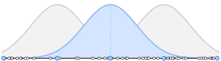
Figure 8: Schema of pre-filtering with σ = 0.2. Raw orientations (white) are convoluted with Gaussian kernel to obtain uniform sampling (blue).

4.3. Regression on SO(3) with normal constraints

To some extent, the pre-filtering smooths out acquisi-tion artifacts in the scanned data. By varying the param-eter σ, it might be possible to sufficiently filter the data while preserving the acquired geometry. However, this approach has a major drawback: since the Gaussian con-volution is applied to each curve individually, there is no guarantee that the filtered orientations will be consistent at intersections (see Sec.3). This type of coherence is how-ever essential, not only for the final reconstruction step of our method (orientations transformed into positional sur-face data) which assumes consistent input, but also to en-sure a correct subsequent processing of the curve network, for instance for surface fitting.

Our goal is therefore to compute a function which is as smooth as possible while fitting the set of frames and satisfying a set of consistency constraints. To have a fil-tering framework with unified representation, our initial idea was to use quaternion splines [Nielson,2004;Park & Ravani,1997;Shoemake,1985]. However, expressing the consistency constraints directly in the quaternion space gives nonlinear equations; on the other hand, these con-straints are linear in SO(3). Inspired by spline functions, which provide smooth curves that reasonably fit the input data by minimizing some energy functional, we propose in the following to formulate filtering of frames (orienta-tions) as a customized energy minimization problem on SO(3).

Recall that a spline in tension x(t) in the d-dimensional Euclidean space Edis the minimizer of the energy

λ ∫ tN t0 ∥x∥˙ 2 dt+ µ ∫ tN t0 ∥¨x∥2 dt

under the interpolation constraints x(ti) = pi ∈ Ed.The

weights λ and µ control stretching and bending of the spline, respectively. Incorporating positional constraints directly in the energy

N ∑ i=0 x(ti) −pi 2 + λ ∫ tN t0 ∥x∥˙ 2 dt+ µ ∫ tN t0 ∥¨x∥2 dt (2)

yields a smoothing spline, useful for non-parametric re-gression and data filtering in Euclidean spaces.

Smoothing splines have been generalized for data on Riemannian manifolds by many authors [Boumal & Absil,

We will now use the manifold formulation to smooth data in the three-dimensional group of rotations which is a Lie group with structure of a differentiable manifold.

Analogically to Euclidean spaces, a smoothing spline X(t) for orientation data Ai∈SO(3) is defined by

minimiz-ing the cost function

N ∑ i=0 dist2 (X(ti),Ai)+λ ∫ tN t0 ⟨_˙ X, ˙X⟩ dt+µ∫ tN t0 ⟨ D2X dt2 , D2X dt2 ⟩ dt, where dist(·, ·) is the Riemannian (geodesic) distance on SO(3), ⟨·, ·⟩ is the Riemannian metric, ˙X is the first deriva-tive and D2X/dt2is the second covariant derivative of X.

We will write the above cost function as E(X) = E0(X) + λE1(X) + µE2(X).

To discretize this problem, the continuous curve X(t) : [0, L] → SO(3)

is replaced by the tensor

γ= (X(t0), . . . ,X(tN)) = (X0, . . . ,XN) ∈SO(3)N+1

where tkis the uniform parametrization defined in (1).

We use the method for spline fitting on manifolds of

Boumal & Absil[2011]. For the sake of completeness, we briefly review the main ideas here. The differential and integral operators in (2) are approximated via geometric fi-nite differences. Geometrically, the difference B − A of two points A, B ∈ Rnin the Euclidean space is the vector

starting at A and pointing towards B whose length is the distance between A and B. On manifolds, the same no-tion is expressed using the Riemannian logarithmic map as log (A⊤B). Note that the logarithmic map is the inverse

of the exponential map, which generates geodesics. For orientation data Ai ∈ SO(3), the cost function (2) has the

following form: N ∑ i=0 log (X ⊤ iAi) 2 F + 1 h N−1 ∑ i=0 log (X ⊤ iXi+1) 2 F + 1 h3 N−1 ∑ i=1 log (X ⊤

iXi+1) +log (X⊤iXi−1)

2 F.

We use the following simplified costs [Boumal,2013]: E0(γ) = N ∑ i=0 ∥Xi−Ai∥ 2 F, E1(γ) = 1 h N−1 ∑ i=0 Xi−Xi+1 2 F, E2(γ) = 1 h3 N−1 ∑ i=1 skew (X ⊤ i (Xi+1+Xi−1)) 2 F, (3)

where γ is the vector of unknown orientations (discrete curve), h = ti− ti−1is the uniform discretization step, and

skew(M) = (M − M⊤)/2. For closed curves, all sums run

from 0 to N due to periodicity.

Let us recall how the simplified energy is obtained. The terms E0,E1 result from the approximation of the

geodesic distance on SO(3) by the chordal distance in the ambient space R3×3: dist2 (A, B) = log (A ⊤_B) 2 F≈ ∥A − B∥2F.

To obtain the simplified term E2, consider the map B 7→

A log (A⊤B), which associates to B ∈ SO(3) a tangent

vec-tor at A ∈ SO(3). A similar vecvec-tor is obtained by project-ing the vector B − A from the ambient space of R3×3to the

tangent space TASO(3). This projection is characterized by the operator A skew(A⊤B). It is therefore convenient

to approximate the log operator by the skew operator: log (A) ≈ skew (A) .

See the paper ofBoumal[2013] for an analysis and the er-ror bounds of the simplified cost.

In our setup, the raw data Aiis associated to a network

Γand the above energy terms are summed over all curves γ ∈Γ. Simultaneously with regression on SO(3), we solve the consistency constraints as follows. Let Xi, ˜Xj be the

local frames of two intersecting curves at their common node η ∈ V. Then the two frames are called consistent, if the frame Xi= [TiBiN] is obtained by rotating the frame

˜ Xj =

[_˜

TjB˜jN] around the surface normal N at the node

η. Denote by N the set of all such pairs (Xi, ˜Xj

)

. To enforce consistency, we add a term penalizing the difference in projection on the normal component

EN(Γ) = ∑ (Xi,˜Xj)∈N Xi|N− ˜Xj|N 2 . (4)

The final energy has the form E (Γ) = ξEN(Γ) +

∑

γ ∈ Γ

E0(γ) + λE1(γ) + µE2(γ) (5)

where ξ, λ, µ ≥ 0 are the weights controlling consistency of surface normals, stretching, and bending, respectively (Fig.16).

The energy E is minimized using the Riemannian region (RTR), a generalization of the classical trust-region in Rn to differentiable manifolds; seeAbsil et al.

[2007] for the description of the algorithm and a detailed convergence analysis. We use the RTR implemented in the ROPTLIB library [Huang et al.,2016].

5. Poisson network reconstruction

In the previous section, we described a filtering method of raw orientation data measured by sensors, which yields uniform, smooth and consistent sampling. We now address the problem of curve network recon-struction under topological constraints: these include in-tersections of two or more curves, and closure of a single curve.

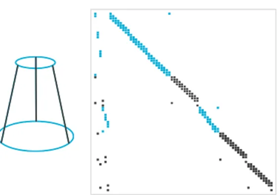
Figure 9: Matrix of the discrete Poisson system (6) for a cone network with two closed curves (blue) and three open curves (black). Dots in-dicate non-zero coefficients. First six columns correspond to network nodes.

Previous approaches treat each curve individually and employ various heuristics to glue the curves together to obtain the correct topology [Hermanis et al., 2016;

Sprynski,2007]. This process is limited to specific (grid) topologies and often requires manual corrections to ob-tain proper intersections. Our approach, on the other hand, naturally satisfies topological constraints by con-struction. In this section, we extend the discretization of the Poisson equation for a single closed curve described byCrane et al.[2013] to curve networks with the topology of a cell complex as defined in Sec.3.

If x is the natural parametrization of the curve γ (one-dimensional Riemannian manifold), the unit tangent field T along γ is equal to the gradient of positions

∇x = T

The vector field T is generally not integrable [Crane et al.,

2013;Kazhdan et al.,2006] and the solution needs to be found in the least-squares sense. To that end, the diver-gence operator is applied to both sides and x is found by solving the Poisson equation

∆x = ∇ · T (6)

Even though the curve network Γ is not a Rieman-nian manifold, it can be viewed as a collection of one-dimensional Riemannian manifolds constrained at inter-sections. This allows us to apply the above Poisson equa-tion to retrieve the network from local orientaequa-tions. With that in mind, we discretize the gradient ∇ and the Lapla-cian ∆ individually for each curve and retrieve the posi-tions by solving a single global linear system. The topo-logical constraints are enforced by representing each node as a unique point in the system (Fig.9).

After the filtering, each curve is represented as a dis-crete collection of unknown points xi = x(ti) ∈ E3, i =

0, . . . , N,with known Darboux frames Xi. We will denote

by Ti = Xi|T the (unit) tangent extracted from Xi. With

uniform parametrization h = ti− ti−1, the differential

op-erators are discretized via finite differences by

∆xi= 1/h2(xi−1−2xi+xi+1) , ∇Ti= 1/h (Ti−Ti−1) .

The above discretization is valid for all interior vertices. At endpoints of open curves, we directly impose the fol-lowing boundary conditions

1/h (x1−x0) =T0,

1/h (xN−xN−1) =TN.

The resulting linear system is sparse with at most three non-zero coefficients per row (Fig.9). Thanks to the re-gression step described in Sec.4.3, the tangent vectors of all curves meeting at network node are coplanar at that node. Therefore the above boundary conditions ensure the reconstruction of a G1 curve network. Note that the

discretization does not take into account the fact that h = ti−ti−1is the geodesic distance along the reconstructed curve,

which differs from the (Euclidean) norm τi = ∥xi−1−xi∥.

In general, this is not an issue, as the least-squares mini-mization of the Poisson energy distributes the error evenly.

Ti

Ti−1

τi

h The euclidean distance τicould be

esti-mated from the geodesic distance h, for in-stance by approximating τiby the chordal

length of the circular arc defined by the length h and angle between Ti−1 and Ti

(see inset). This estimation comes at a price – the modified parametrization is no longer uniform. Our experiments have shown that the error |τi− h| is generally

too small to influence the reconstruction. 6. Evaluation

6.1. Data acquisition

To acquire data on physical surfaces, we use dynamic acquisition setup – the orientations are measured using a single IMU, which is moved around on the surface by the user. In our experiments we used two types of de-vices: a standard smartphone, and a custom-made device. The Morphorider (Fig.10) is a wireless mouse-like device for measuring local orientation, containing a single 3A3M sensor (a tri-axial accelerometer and a tri-axial magne-tometer) with an incremental wheel for tracking distance. It is a prototype specifically designed for acquisition of curves on surfaces. 12cm 7cm r−= −14cm r+= +9cm r−= −9cm r+= +4cm

Figure 10: Left: the Morphorider and the wireless keypad used for mark-ing nodes durmark-ing acquisition. Right: the schema shows limitations of the device with respect to radius of curvature at locally convex (red) and concave (blue) surface points.

We use a MATLAB interface to acquire data with the Morphorider (Fig.11left). Prior to acquisition, we assign a unique index between 0 and n − 1 to each of the n net-work nodes. The acquisition is controlled remotely using

a wireless numpad (Fig. 10 left). When starting a new curve, we first indicate if the curve is at the boundary or in the interior. Then, every time the device passes through a node, we record its index. See the accompanying video for the acquisition setup.

Figure 11: The devices used for data acquisition. Left: the Morphorider (a custom-made device) and a screenshot of the MATLAB acquisition in-terface. Right: a standard smartphone and the application with a simple acquisition interface.

Similarly, orientation data can be measured with a standard smartphone. In addition to accelerometers and magnetometers, smartphones also contain gyroscopes. This enables orientation acquisition that is more robust to magnetic perturbations. We use the state of the art sensor fusion algorithms to robustly estimate orientation from sensor measurements [Madgwick et al.,2011;Pacha,

2013]. However, measuring distances with a smartphone is difficult. The GPS is not an option for mid-sized objects such as the lilium (Fig.11) whose bounding box has di-mensions 1.00m×1.00m×0.25m. To overcome this limita-tion, we assume the speed of acquisition is constant, then we parametrize each curve using acquisition timestamps. Optionally, manual distance measurements can be used to increase the precision of reconstruction. We measure the length Ls for each segment s which is then used to

transform the time parameter t ∈ [tstart, tend]into the nat-ural parameter d ∈ [0, Ls]. In this case, we suppose the

speed of acquisition is constant for each segment, but it does not need to be constant through the whole acquisi-tion process. In practice, the constant-speed-per-segment constraint is much easier to handle and the manual dis-tance measurement improves the reconstruction (Fig.12). To acquire data with a smartphone, we use a lightweight Java application (Fig.11right).

6.2. Convergence and error of reconstruction

We demonstrate the performance of our reconstruc-tion framework on synthetic and acquired data.

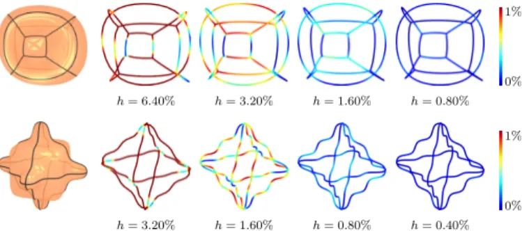
• We use synthetic data extracted from known ground truth networks for convergence analysis of the Pois-son network reconstruction (Fig.13). The synthetic data are not corrupted by noise and therefore do not need to be filtered.

• Data acquired from known surfaces serve for evalu-ating the overall performance of the framework on real-world examples (Fig. 14 and 15). Moreover, they enable quantitative comparison of the two ac-quisition methods. Morphorider distance param. measured lengths smartphone time param. measured lengths smartphone time param. estimated lengths

e_{mean = 1.15%} e_{mean = 0.78%} e_{mean = 2.11%} 0% 4%

Figure 12: Comparison of three acquisition setups for the lilium. Top pictures show surfaced networks rendered with reflection lines; bottom pictures show the error of Poisson reconstruction for each network. In the left network, the orientations were acquired using the Morphorider and parametrized by distances. In middle and right networks, the ori-entations were acquired with the smartphone and parametrized by ac-quisition time – middle network uses measured segment lengths, right network uses time-estimated segment lengths. All lengths are relative to the diameter (length of AABB diagonal) of the ground truth surface.

0% 1% h= 6.40% h= 3.20% h= 1.60% h= 0.80% 0% 1% h= 3.20% h= 1.60% h= 0.80% h= 0.40% Figure 13: As h → 0, synthetic networks reconstructed by solving the Poisson equation (6) converge to the ground truth network (black). All lengths are relative to the diameter (length of AABB diagonal) of the ground truth surface (orange).

The error metric associated with each point x in the re-constructed network is defined as the distance between x and its closest point on the ground truth network or sur-face. For synthetic data, the closest point is found on the ground truth network. For data acquired from a physical surface with a known digital model (lilium, cone), closest points are instead found on the underlying surface as the ground truth network is not available. Note that the di-mensions of the fabricated surfaces are 1.00m × 1.00m × 0.25m (lilium) and 1.00m × 1.00m × 2.00m (cone). Prior to error computation the acquired network needs to be reg-istered to the surface, since the two objects do not live in the same coordinate systems. We use the ICP algorithm [Besl & McKay,1992] for the registration.

The convergence plot for decreasing h is shown in Fig. 17 and the corresponding numerical data is given in Table 1. All errors are relative to the diameter (the length of AABB diagonal) of the corresponding ground truth surface. For synthetic data (bowl, bumpycube), the

mrider

h= 6.40% h= 3.20% h= 1.60% h= 0.80% h= 0.40%

smartphone

0% 4%

Figure 14: Reconstruction error for the lilium scanned with the Mor-phorider (top) and a smartphone (bottom) for decreasing h. For filtering, we used the weights λ = µ = 1. All lengths are relative to the diameter (length of AABB diagonal) of the ground truth surface.

h= 6.40% h= 3.20% h= 1.60% h= 0.80% h= 0.40% fitted surface 0% 2%

Figure 15: Reconstruction error for the cone scanned with the Mor-phorider for decreasing h. For filtering, we used the weights λ = µ = 1. All lengths are relative to the diameter (length of AABB diagonal) of the ground truth surface.

mean error approaches zero for decreasing h (Fig. 13). For acquired networks on the lilium, the mean error is about 1% using measured distances (both devices) and around 2% using time-estimated distances (smartphone). It is not surprising that when using the measured dis-tances, the smartphone error decreases faster than the Morphorider error. One can further observe that even though the smartphone error (both mean and max) is big-ger than the Morphorider error at coarser resolutions, it becomes smaller at finer scales. We explain this behav-ior by the fact that the distance data are not the same for the two devices. For the Morphorider data, we have exact correspondences between distance and orientation mea-surements; for the smartphone data, only the total length of each segment is known and the correspondences are es-timated from acquisition time. It seems like at finer scales, the error of this estimation is better-distributed, which re-sults in a reconstruction with higher precision.

6.3. Filtering

The main goal of the filtering algorithm described in Sec.4 is to obtain clean and consistent orientations from raw sensor measures. The weights λ, µ in the filtering en-ergy (5) influence the shape of the reconstructed network indirectly by controlling stretching and bending of splines on the manifold SO(3) used for orientation smoothing. In all examples, we use the weight ξ =1e4 to enforce the con-sistency of normals.

The influence of λ and µ on the Poisson-reconstructed positions is compared in Fig. 18. Interestingly, even though λ and µ control stretching and bending of

orienta-tions Xi, they also seem to control stretching and bending

of reconstructed positions xi. The weights need to be

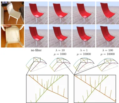
cho-no filter λ = 10 λ = 1 λ = 100 µ = 1000 µ = 10000 µ = 10000

Figure 16: A chair reconstructed with different sets of weights. After the pre-filtering, normals at nodes are not compatible (bottom left). The normal penalty term in the filtering energy ensures the consistency of the reconstructed network (bottom right).

sen carefully, otherwise the network might end up over-filtered; see Fig.18where λ = 100.

6.4. Additional results

To further illustrate the benefits of our method, we compute smooth surfaces that fit not only the resulting network of curves but also the corresponding filtered sur-face normals using the algorithm ofStanko et al.[2016]. All other fitting techniques that take into account the nor-mal vectors available along the curve network [Botsch & Kobbelt,2004; Jacobson et al.,2010] could also be used. Fig.20shows some of the reconstructed surfaces.

Fig.16shows surfaces interpolating the chair network filtered with various sets of weights. It also illustrates the phenomenon of inconsistent orientations: pre-filtered normals do not agree at intersections, and naive averaging of each pair of conflicting normals results in a shape with poor fidelity to the scanned object (Fig.16 bottom left). Our regression filtering technique resolves this problem while preserving the underlying geometry (Fig.16bottom right). Note however that surface reconstruction is not in the scope of this paper.

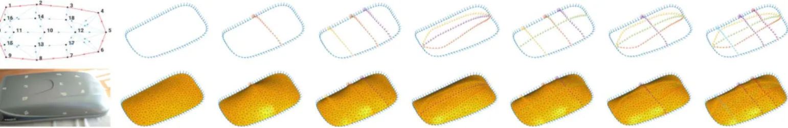
During acquisition, we often faced the question of what curves to acquire in order to minimize the error of reconstruction – different curve networks on the same sur-face often produce different results. Fig.19shows the roof box reconstructed with seven different sets of curves. The optimal choice of curves to be scanned merits to be inves-tigated futher, but goes beyond the scope of the paper.

0.4% 0.8% 1.6% 3.2% 6.4% 0.0% 1.0% 2.0% 3.0%

cone lilium phone lilium mrider bumpycube bowl

Figure 17: Reconstruction error with respect to ground truth. Abscis-sae is step size relative to object size. Solid lines represent mean error (Table1), while dashed lines represent maximal error. All lengths are relative to the diameter (length of AABB diagonal) of the ground truth surface.

data source lengths mean error (%) h (%) 6.4 3.2 1.6 0.8 0.4 bowl synth. exact 1.11 0.53 0.24 0.10 -bumpy synth. exact - 1.60 0.55 0.19 0.08

cone mrider measured 0.61 0.49 0.46 0.45 0.45 lilium mrider measured 1.36 1.23 1.19 1.17 1.15 lilium phone measured 1.94 1.38 0.89 0.81 0.78 lilium phone time-est. - 1.83 2.01 2.03 2.11 Table 1: Mean distance error with respect to ground truth. All lengths are in % and relative to the diameter (length of AABB diagonal) of the corresponding ground truth surface.

7. Limitations and future work

Most limitations of our method are device-related. The current Morphorider is a proof of concept and suf-fers from construction drawbacks. Its relatively big size inhibits the acquisition; we often found it hard to manip-ulate, and some regions with high curvature (in absolute value) could not have been scanned (see Fig. 10). An-other problem is that the distance-measuring wheel is not aligned with the sensor unit – in practice this means that there is an offset in the orientation measurement. More-over, the device relies on magnetometers and cannot be used around ferromagnetic objects. A next generation prototype currently in development might help in resolv-ing some of these problems. The biggest limitation of the smartphone setup is the inability to measure distances – these need to be estimated or obtained manually.

The current approach requires the user to have a spe-cific network topology in mind prior to the acquisition. Nodes cannot be added during acquisition – adding a new node means that all previously scanned curves passing through this node need to be re-scanned, which is imprac-tical and slows down the scanning process. Moreover, the system needs user feedback to know when the acquisition device passes through a node. In future, we plan to im-plement a more intuitive interface by using a heuristic for snapping curves to existing nodes to ease the acquisition. Curvature plots in Fig.18imply that the reconstructed curves are G2, but there are issues with overall G2

-continuity at nodes. We believe these issues might be re-solved by a slight modification of the normal penalty term in the filtering energy, for instance by taking into account normals of node’s neighboring vertices. We also plan to extend the method to surfaces with sharp features, i.e. curves with two sets of frames that agree up to rotation around curve’s tangent vector.

Acknowledgments. This research was partially funded by the ERC advanced grant no. 291184 EXPRESSIVE.

References

Absil, P.-A., Baker, C., & Gallivan, K. (2007). Trust-region methods on riemannian manifolds. Foundations of Computational Mathematics, 7(3), 303–330.

Andrews, J., Joshi, P., & Carr, N. (2011). A linear variational system for modelling from curves. Computer Graphics Forum, 30(6), 1850–1861. Antonya, C., Butnariu, S., & Pozna, C. (2016).Real-time representation of

the human spine with absolute orientation sensors. In 14th Int. Conf.

on Control, Automation, Robotics and Vision (ICARCV) (pp. 1–6).

Arora, R., Kazi, R. H., Anderson, F., Grossman, T., Singh, K., & Fitzmau-rice, G. (2017). Experimental evaluation of sketching on surfaces in vr. In Proc. Conf. Human Factors in Computing Systems (CHI). ACM. Bae, S.-H., Balakrishnan, R., & Singh, K. (2008). ILoveSketch:

As-Natural-As-Possible Sketching System for Creating 3D Curve Models. In UIST ’08 (pp. 151–160). ACM.

Berberich, E., Fogel, E., Halperin, D., Mehlhorn, K., & Wein, R. (2010).

Arrangements on Parametric Surfaces I: General Framework and In-frastructure. Mathematics in Computer Science, 4, 45–66.

Besl, P., & McKay, N. (1992). A method for registration of 3-D shapes.

Trans. Pattern Analysis and Machine Intelligence, 14, 239–256.

Botsch, M., & Kobbelt, L. (2004). An intuitive framework for real-time freeform modeling. ACM Trans. Graph. (Proc. SIGGRAPH), 23(3), 630– 634.

Boumal, N. (2013).Interpolation and regression of rotation matrices. In F. Nielsen, & F. Barbaresco (Eds.), Geometric Science of Information (pp. 345–352). Springer Berlin Heidelberg volume 8085 of Lecture Notes in

Computer Science.

Boumal, N., & Absil, P.-A. (2011).A discrete regression method on man-ifolds and its application to data on SO(n). In Proceedings of the 18th

IFAC World Congress (Milan) (pp. 2284–2289). volume 18.

Boumal, N., Mishra, B., Absil, P.-A., & Sepulchre, R. (2014). Manopt, a Matlab toolbox for optimization on manifolds. Journal of Machine

Learning Research, 15, 1455–1459.

Brunnett, G., & Crouch, P. E. (1994). Elastic curves on the sphere.

Ad-vances in Computational Mathematics, 2(1), 23–40.

Cao, Y., Nan, L., & Wonka, P. (2016). Curve networks for surface recon-struction. preprint, .http://arxiv.org/abs/1603.08753.

Coons, S. A. (1967). Surfaces for computer-aided design of space forms. Tech-nical Report DTIC Document.

Crane, K., Pinkall, U., & Schröder, P. (2013).Robust fairing via conformal curvature flow. ACM Trans. Graph. (Proc. SIGGRAPH), 32.

Crassidis, J. L., Markley, F. L., & Cheng, Y. (2007). Survey of nonlinear attitude estimation methods. Journal of guidance, control, and dynamics,

30(1), 12–28.

Farin, G. E. (2002). Curves and surfaces for CAGD: a practical guide . (5th ed.). Morgan Kaufmann.

Google (2017). Tilt Brush.https://www.tiltbrush.com/. Hatcher, A. (2002). Algebraic Topology. Cambridge University Press. Hermanis, A., Cacurs, R., & Greitans, M. (2016).Acceleration and

mag-netic sensor network for shape sensing. IEEE Sensors Journal, 16(5), 1271–1280.

no filter λ = 1 µ = 1 λ = 100 µ = 1 λ = 1 µ = 100 λ = 100 µ = 100

Figure 18: Reconstruction of lilium with various filtering weights. Left to right in each row: reconstructed network with porcupine plot (surface normal scaled by curvature); Gauss map; curvature plot.

Figure 19: Surface of a roof box reconstructed with different sets of curves.

Hofer, M., & Pottmann, H. (2004). Energy-minimizing splines in mani-folds. ACM Transactions on Graphics (TOG), 23(3), 284–293.

Hoshi, T., & Shinoda, H. (2008). 3D Shape Measuring Sheet Utilizing Gravitational and Geomagnetic Fields. In SICE Annual Conference (pp. 915–920).

Huang, W., Absil, P.-A., Gallivan, K. A., & Hand, P. (2016). ROPTLIB:

an object-oriented C++ library for optimization on Riemannian manifolds.

Technical Report FSU16-14.v2 Florida State University.http://www. math.fsu.edu/~whuang2/papers/ROPTLIB.htm.

Huard, M., Sprynski, N., Szafran, N., & Biard, L. (2013).Reconstruction of quasi developable surfaces from ribbon curves. Numerical

Algo-rithms, 63(3), 483–506.

Igarashi, T., Matsuoka, S., & Tanaka, H. (1999). Teddy: A Sketching In-terface for 3D Freeform Design. In Proc. SIGGRAPH 99. Annual

Con-ference Series (pp. 409–416).

InstruMMents (2017). 01 dimensioning instrument. http:// instrumments.com/.

Jacobson, A., Tosun, E., Sorkine, O., & Zorin, D. (2010). Mixed Finite Elements for Variational Surface Modeling. Computer Graphics Forum

(Proc. SGP), 29(5), 1565–1574.

Kazhdan, M., Bolitho, M., & Hoppe, H. (2006). Poisson Surface Recon-struction. In Proc. SGP (pp. 61–70).

Madgwick, S., Harrison, A., & Vaidyanathan, R. (2011). Estimation of IMU and MARG orientation using a gradient descent algorithm. In

IEEE Int. Conf. Rehabilitation Robotics (pp. 1–7).

Markley, F. L., Cheng, Y., Crassidis, J. L., & Oshman, Y. (2007).Averaging quaternions. Journal of Guidance, Control, and Dynamics, 30(4), 1193– 1197.

Markley, F. L., & Mortari, D. (2000). Quaternion attitude estimation using vector observations. Journal of the Astronautical Sciences, 48(2), 359–380. Milosevic, B., Bertini, F., Farella, E., & Morigi, S. (2016). A SmartPen for 3D interaction and sketch-based surface modeling. The International

Journal of Advanced Manufacturing Technology, 84(5), 1625–1645.

Moreton, H. P., & Séquin, C. H. (1991). Surface Design with Minimum Energy Networks. In Proc. ACM/SIGGRAPH Symposium on Solid

Mod-eling and CAD/CAM Applications (pp. 291–301).

Nealen, A., Igarashi, T., Sorkine, O., & Alexa, M. (2007).FiberMesh: De-signing Freeform Surfaces with 3D Curves. ACM Trans. Graph. (Proc.

SIGGRAPH), 26(3).

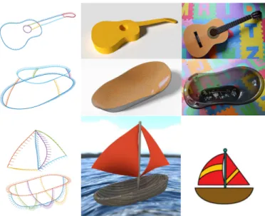
Figure 20: Top: guitar and bathtub scanned using the Morphorider. Left to right, reconstructed networks, surfaces computed from the networks, the scanned objects. The guitar shape was created by extruding the sur-faced network. Scanning the translucent bathtub was not an issue. Bottom: inspired by the image on the right, we created a 3D model of the sailboat by sketching the network on the left with a smartphone. The lengths were estimated from time of acquisition.

of orientations. IEEE Trans. Vis. Comput. Graphics, 10, 224–229. Pacha, A. (2013). Sensor Fusion for Robust Outdoor Augmented Reality

Tracking on Mobile Devices. Master’s thesis.

Park, F. C., & Ravani, B. (1997). Smooth invariant interpolation of rota-tions. ACM Trans. Graph., 16(3), 277–295.

Reinsch, C. H. (1967).Smoothing by spline functions. Numerische

Math-ematik, 10(3), 177–183.

Saguin-Sprynski, N., Carmona, M., Jouanet, L., & Delcroix, O. (2016). New generation of flexible risers equipped with motion capture – Morphopipe system. In EWSHM – 9th European Workshop on

Struc-tural Health Monitoring.

Saguin-Sprynski, N., Jouanet, L., Lacolle, B., & Biard, L. (2014). Surfaces Reconstruction Via Inertial Sensors for Monitoring. In EWSHM – 7th

European Workshop on Structural Health Monitoring.

Shoemake, K. (1985).Animating rotation with quaternion curves.

Com-puter Graphics, 19(3), 245–254. Proc. SIGGRAPH.

Sprynski, N. (2007). Reconstruction de courbes et de surfaces à partir de

don-nées tangentielles. PhD thesis, Université de Grenoble.

Sprynski, N., Szafran, N., Lacolle, B., & Biard, L. (2008). Surface

re-construction via geodesic interpolation. Computer Aided Design, 40(4), 480–492.

Stanko, T., Hahmann, S., Bonneau, G.-P., & Saguin-Sprynski, N. (2016).

Surfacing curve networks with normal control. Computers & Graphics,

60, 1–8.

Xu, B., Chang, W., Sheffer, A., Bousseau, A., McCrae, J., & Singh, K. (2014).True2form: 3d curve networks from 2d sketches via selective regularization. ACM Trans. Graph. (Proc. SIGGRAPH), 33(4), 131:1– 131:13.

data _rawsamples_{uni conv.} time (ms)_{regress. Poisson} mushroom Fig.2 831 508 10 202 8 lilium Fig.14 top 3243 96 3 51 1 196 6 113 3 382 6 234 7 742 9 439 30 1416 15 788 170 lilium Fig.14 bottom 531 99 3 28 2 186 6 55 3 362 8 83 10 713 11 192 31 1420 16 428 172 cone Fig.15 949 205 5 176 3 398 3 328 8 783 8 618 28 1553 14 1169 136 3094 22 2779 904 chair Fig.16 584 247 3 592 6 1315 1461 lilium Fig.18 3243 428 7 125 10 319 517 522

Table 2: Performance of the algorithm implemented in C++ using ROPTLIB on a standard quad-core CPU computer. The stats include number of raw samples, number of uniform samples, Gaussian convo-lution time, SO(3) regression time, Poisson network reconstruction time. All timings are in milliseconds.