HAL Id: hal-00582039
https://hal.archives-ouvertes.fr/hal-00582039
Submitted on 1 Apr 2011
HAL is a multi-disciplinary open access archive for the deposit and dissemination of sci-entific research documents, whether they are pub-lished or not. The documents may come from teaching and research institutions in France or abroad, or from public or private research centers.
L’archive ouverte pluridisciplinaire HAL, est destinée au dépôt et à la diffusion de documents scientifiques de niveau recherche, publiés ou non, émanant des établissements d’enseignement et de recherche français ou étrangers, des laboratoires publics ou privés.
Mohamed Jellal, Christophe Jalil Nordman, Francois-Charles Wolff
To cite this version:
Mohamed Jellal, Christophe Jalil Nordman, Francois-Charles Wolff. Evidence on the glass ceiling effect in France using matched worker-firm data. Applied Economics, Taylor & Francis (Routledge), 2008, 40 (24), pp.3233-3250. �10.1080/00036840600994070�. �hal-00582039�
For Peer Review
Evidence on the glass ceiling effect in France using matched worker-firm data
Journal: Applied Economics Manuscript ID: APE-06-0005.R1 Journal Selection: Applied Economics
JEL Code:
J16 - Economics of Gender < J1 - Demographic Economics < J - Labor and Demographic Economics, J31 - Wage Level, Structure; Differentials by Skill, Occupation, etc. < J3 - Wages, Compensation, and Labor Costs < J - Labor and Demographic Economics, J24 - Human Capital|Skills|Occupational Choice|Labor Productivity < J2 - Time Allocation, Work Behavior, and Employment
Determination/Creation < J - Labor and Demographic Economics Keywords: gender wage gap, glass ceiling, quantile regressions, matched worker-firm data
For Peer Review
Evidence on the glass ceiling effect in France
using matched worker-firm data
#Mohamed JELLAL*, Christophe NORDMAN** and François-Charles WOLFF***
Applied Economics, first revision
June 2006Abstract: In this paper, we investigate the relevance of the glass ceiling hypothesis in France, according to which there exist larger gender wage gaps at the upper tail of the wage distribution. Using a matched worker-firm data set of about 130,000 employees and 14,000 employers, we estimate quantile regressions and rely on a principal component analysis to summarize information specific to the firms. Our different results show that accounting for firm-related characteristics reduces the gender earnings gap at the top of the distribution, but the latter still remains much higher at the top than at the bottom. Furthermore, a quantile decomposition shows that the gender wage gap is mainly due to differences in the returns to observed characteristics rather than in differences in characteristics between men and women.
JEL Classification: J24, J31, J16
Keywords: gender wage gap; glass ceiling; quantile regressions; matched worker-firm data
# We would like to thank seminar participants at DIAL, INED and LEST for helpful suggestions. We have also
benefited from the constructive comments and remarks of an anonymous referee. Any remaining errors are ours.
* Université Mohammed V, Rabat, Morocco ; and Conseils-Eco, 10 impasse de Mansencal, 31500 Toulouse, France.
E-mail : [email protected]
** Corresponding author. DIAL, IRD, Paris. 4 rue d'Enghien, 75010 Paris, France. E-mail: [email protected] *** LEN, Université de Nantes, BP 52231 Chemin de la Censive du Tertre, 44322 Nantes Cedex, France ; CNAV and
INED, Paris, France. E-mail: [email protected] http:\\www.sc-eco.univ-nantes.fr\~fcwolff
3 4 5 6 7 8 9 10 11 12 13 14 15 16 17 18 19 20 21 22 23 24 25 26 27 28 29 30 31 32 33 34 35 36 37 38 39 40 41 42 43 44 45 46 47 48 49 50 51 52 53 54 55 56 57 58 59 60
For Peer Review
1. Introduction
The persistence of wage differentials between men and women with identical productive characteristics is an important stylised fact of labour markets in both industrialised and developing countries. Evidence of a gender wage gap in pay is indeed abundant. Wage differentials across genders that are not compensated by observed socio-economic characteristics were found on numerous occasions in empirical studies (see for instance the review in Blau and Kahn, 2000). Many models have attempted to give a theoretical interpretation to these gender pay gaps. Traditionally, economists have focused on either qualifications or labour market treatment of similarly qualified individuals1. Other theories like the insider-outsider or the efficiency wage
models have stressed non-competitive mechanisms of wage determination.
More recently, it has been suggested that there exist larger gender wage gaps at the upper tail of the wage distribution, so that it concerns in most cases the more skilled workers. This is the so-called glass ceiling effect above women in the labour market, which can be defined as an invisible barrier that inhibits promotion opportunities for women, but not for men, and prevents them from reaching top positions. Several papers have empirically shed light on the magnitude of the glass ceiling effect in different European countries2.
For instance, using data collected in 1998 in Sweden, Albrecht et al. (2003) show that the gender wage gap is increasing throughout the conditional wage distribution and accelerating at the top, and they interpret this result as evidence of a glass ceiling in Sweden. Using data for Spain, De la Rica et al. (2005) stratify their sample by education group and find that the gender wage gap is expanding over the wage distribution only for the group with tertiary education. For less educated groups, the gender wage gap is wider at the bottom than the top. This means that, in Spain, there is a glass ceiling for the more educated, while for the less educated there is not.
1 The former, within the competitive framework, emphasise the existence of compensating wages due, for instance,
to differences in human capital accumulation across gender. Because women anticipate shorter and more discontinuous work lives, they have lower incentives to invest in market-oriented formal education and on-the-job training, and their resulting smaller human capital investments will lower their earnings relative to those of men.
3 4 5 6 7 8 9 10 11 12 13 14 15 16 17 18 19 20 21 22 23 24 25 26 27 28 29 30 31 32 33 34 35 36 37 38 39 40 41 42 43 44 45 46 47 48 49 50 51 52 53 54 55 56 57 58 59 60
For Peer Review
Using the European Community Household Panel data set, Arulampalam et al. (2004) find that for most of their ten EU countries, in both the public and private sectors, the average gender wage gap can be broken up into a gap that is typically wider at the top and occasionally also wider at the bottom of the conditional wage distribution. They interpret the gender wage gap at the top of the wage distribution as a glass ceiling evidence, whereby women otherwise identical to men can only advance so far up the pay ladder. At the bottom of the wage distribution in some of their EU countries, they also find that the gender pay gap widens significantly and define this phenomenon as a sticky floor (see also Booth et al., 2003; Ichino and Filippin, 2005).
Surprisingly, to date, there is no clear theoretical argument to rationalize the glass ceiling effect among the various usual existing explanations for the gender wage gap. According to the beckerian theory, discrimination is due to the discriminatory tastes of employers, co-workers, or customers. Alternatively, in models of statistical discrimination, differences in the treatment of men and women arise from average differences between the two groups in the expected value of productivity or in the reliability with which productivity may be predicted, which lead employers to discriminate on the basis of that average. Discriminatory exclusion of women from ‘male’ jobs can also result in an excess supply of labour in ‘female’ occupations, depressing wages there for otherwise equally productive workers. But in these various approaches, there is no reason to expect larger gaps at the upper tail of the wage distribution.
De la Rica et al. (2005) suggest that a dead-end argument operate in the upper tail of the distribution3. Women are less frequently promoted because their jobs can less easily be promoted.
Employees are most often reluctant to invest in women’s training, for instance because women have more favourable outside opportunities than men within the household. Jellal et al. (2005) introduce uncertainty on the female productivity in a competitive labour market model. Women 2 Conversely, evidence on gender-earnings differentials in less developed countries remains scarce. See for instance
Sakellariou (2004) for quantile wage regressions in the Philippines, Hinks (2002) in South Africa or Nielsen (2000) in Zambia. 3 4 5 6 7 8 9 10 11 12 13 14 15 16 17 18 19 20 21 22 23 24 25 26 27 28 29 30 31 32 33 34 35 36 37 38 39 40 41 42 43 44 45 46 47 48 49 50 51 52 53 54 55 56 57 58 59 60
For Peer Review
are likely to have more frequently interrupted careers (because of birth event for instance), and they may choose to quit the labour force either to spend time with children or to care for elderly parents. Owing to this uncertainty, firms pass the risk of variability in women’s production on female wages and the negative risk premium increases as women are more qualified.
In this paper, we wonder whether it matters to control for firms’ characteristics when estimating the gender wage gap along the wage distribution. Our contribution is thus mainly empirical, as we do not propose any economic hypotheses related to firm characteristics. This is undoubtedly a shortcoming of the present analysis, but the difficulty is that several explanations may be invoked to rationalize the glass ceiling effect. Furthermore, it may be excessively difficult to assess the relevance of these hypotheses4. Thus, our paper may be seen as a first step in the
inclusion of firms’ characteristics in the gender wage gap and glass ceiling literature, with a focus on empirical assessment. The next step would be naturally to further investigate the influence of these firms’ factors in order to get a comprehensive understanding on the glass ceiling effect.
So, we primarily assess the relevance of the glass ceiling hypothesis using matched worker-firm data collected in 1992 in France. Although differences in productivity across workers could stem from their differences in human capital, it is well acknowledged that some skills or human capital attributed to workers are also specific to the firms in which those workers operate. Thus, part of the returns to human capital for the worker remuneration can be viewed as originating from the firm (see Abowd et al., 1999)5. Hence, not controlling for firm specific
effects on individual earnings differentials may lead to biased estimates when focusing on returns to human capital by gender. Curiously, firm specific effects have been neglected so far in the 3 Conversely, since high-educated women have participation rates which are only slightly lower than male
participation rates, women’s and men’s wages should not be very different in the lower part of the income distribution (De la Rica et al., 2005).
4 This is the case for instance for the uncertainty argument suggested by Jellal et al. (2005). The French data provides
very poor proxy on the measure of uncertainty. Also, finding some results in favor of the uncertainty argument does not preclude that the motivation for the glass ceiling effect is due to other arguments not specifically related to uncertainty considerations.
5 It is also possible that part of what could be interpreted as human capital externalities in the estimates is in fact a
consequence of the selection of workers by firms and vice versa. For instance, highly educated workers (i.e. high wage workers) are more likely to match with high wage firms (Abowd et al., 1999).
3 4 5 6 7 8 9 10 11 12 13 14 15 16 17 18 19 20 21 22 23 24 25 26 27 28 29 30 31 32 33 34 35 36 37 38 39 40 41 42 43 44 45 46 47 48 49 50 51 52 53 54 55 56 57 58 59 60
For Peer Review
analysis of gender earnings gap, Bayard et al. (2003) and Meng (2004) being worthwhile exceptions.
As a consequence, the gender wage gap at the upper tail of the wage distribution may be wrongly overstated if firms reward highly educated women differently than men. Thus, our main contribution is to propose for the first time an empirical investigation of the glass ceiling effect in a context where specific firm effects are controlled for. Following previous studies, we first use quantile regressions techniques to assess the extent to which the glass ceiling phenomenon exists in France. Then, we control for firms’ specific wage policies by introducing the firms’ features into the different earnings functions. A novelty of our approach is to perform quantile regressions using a preliminary principal component analysis of firms’ characteristics, as in Muller and Nordman (2004, 2005). We also carry out a quantile decomposition analysis with the inclusion of firms’ factors. We follow the method of Machado and Mata (2005) and examine whether gender wage differences stem from differentiated returns to observable characteristics.
In France, we find that introducing firm-related characteristics into earnings equation significantly reduces the gender earnings gap at the top of the distribution. However, the gender wage gap still remains greater at the top than at the bottom as in other European countries. The rest of the paper is organized as follows. In Section 2, we describe the French ECMOSS survey conducted in 1992 by INSEE. In Section 3, we present the econometric methodology and our strategy to account for firm related characteristics. We discuss in Section 4 the different results of the quantile regressions along with results from the quantile decomposition. Section 5 concludes.
2. The French matched worker-firm data
The data we use in this paper are drawn from a unique French survey which matches information of both employers and employees, the 1992 INSEE survey on labour cost and wage structure (Enquêtes sur le Coût de la Main-d'Oeuvre et la Structure des Salaires en 1992, ECMOSS thereafter). It is well known that such data sets allow the structure of wages to be modelled while
3 4 5 6 7 8 9 10 11 12 13 14 15 16 17 18 19 20 21 22 23 24 25 26 27 28 29 30 31 32 33 34 35 36 37 38 39 40 41 42 43 44 45 46 47 48 49 50 51 52 53 54 55 56 57 58 59 60
For Peer Review
controlling for firm-specific effects (see Abowd et al., 1999). Specifically, the French survey contains information on 150,000 different workers across 16,000 different workplaces6. The
sampling population covered by these data is very broad, as all establishments are covered independently of their size and in all industries apart from agriculture, fisheries, non-traded services, and central and local government.
The ECMOSS survey contains a great deal of information. Concerning the employees, data are available on workers' gross annual wage, which is broken down into fixed salary, bonuses, overtime, and data on their gender, age, nationality, tenure, occupation, education level and number of paid hours. There is also some detailed information on the employer, including main economic activity, size, geographical location, management style, work organisation and salary policy. In order to perform our econometric analysis, several additional variables have been constructed and we describe them below.
Concerning the workers, we determine the total number of years of education calculated from the final level reached, total potential experience in the labour market which is given by age minus number of years of education minus six, hourly earnings (gross salary plus payments in kind, all divided by the number of paid hours over the year), and the average number of paid hours of training per worker in the establishment (the number of hours of paid training by worker by occupational category – executive or non-executive – divided by the total number of workers by occupational category) 7.
By definition, we have only information on persons having a paid job in the French matched data set. This is undoubtedly a shortcoming as we are unable to account for gender differences in the labour force participation. It is well known that women have a lower probability
6 This labour cost survey is concurrently carried out in all European Union countries every four years and aims at
providing comparable labour market statistics across EU countries. In the 1992 wave of this survey, INSEE matched the data with those on the wage structure. For previous studies which have estimated earnings functions on the same data, see among others Abowd et al. (2001), Destré and Nordman (2002), Destré (2003) and Meng and Meurs (2004).
7 The education variable is constructed as follows. For a sub-sample of more than 8000 workers for whom the
number of years of education is available (besides the highest paper certificate), we calculate the median number of years of education for each qualification considered. This indirect method for calculating the length of education has the advantage of partially removing the endogeneity of the education variable (see the discussion in Destré, 2003).
3 4 5 6 7 8 9 10 11 12 13 14 15 16 17 18 19 20 21 22 23 24 25 26 27 28 29 30 31 32 33 34 35 36 37 38 39 40 41 42 43 44 45 46 47 48 49 50 51 52 53 54 55 56 57 58 59 60
For Peer Review
to take part in the labour market, which raises some selectivity issue. Albeit the expected positive self-selection for women that may affect the magnitude of the gender wage gap, the problem is certainly not too severe. The selection issue has been recently addressed within a quantile decomposition framework by Albrecht et al. (2006). In the Netherlands, these authors evidence a positive self-selection of women into full-time work, but still find that the bulk of the gender wage gap is due to differences between men and women in the return to individual characteristics. In the same way, again owing to data limitation, we focus on workers currently employed in the private sector. Again, this restriction leads to a selection bias as women tend to be more present in the public sector. Nevertheless, in the French context, the problem is certainly less severe than it seems owing to the fact that, in the public sector, wages are mainly fixed by law and then cannot really respond to productivity or discrimination strategies. After deleting observations with missing values or outliers, the worker sample amounts to 137,211 individuals divided into 14,693 establishments. Table 1 provides a description of the characteristics of the employees.
Insert Table 1 about here
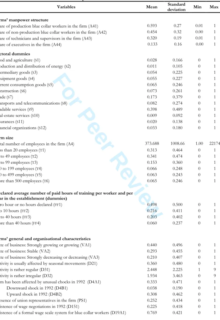
To test the glass ceiling hypothesis, one novelty of our approach is to control for firm level variables in the analysis of wage determination. We describe below the information that is utilised for a preliminary multivariate analysis of firm-related characteristics. The definitions and descriptive statistics of these variables appear in Table A of the Appendix.
First, we make use of twelve sectoral dummies (S1, S2, S3, S4, S5, S6, S7, S8, S9, S10, S11,
S12), the size of the establishments (A4)8, and four dummies for the average number of paid hours of training per worker in the establishment (in increasing order, FF1, FF2, FF3, FF4). The following variables relate to qualitative aspects of firms’ activity: dummies describing the intensity of business the past five years (“strongly growing” or “growing”: VA1, “stable”: VA2; “strongly decreasing” or “decreasing”: VA3), whether activity is usually affected by seasonal movements
3 4 5 6 7 8 9 10 11 12 13 14 15 16 17 18 19 20 21 22 23 24 25 26 27 28 29 30 31 32 33 34 35 36 37 38 39 40 41 42 43 44 45 46 47 48 49 50 51 52 53 54 55 56 57 58 59 60
For Peer Review
(D21), whether it is rather regular (D31), or irregular (D32), whether firms have been affected by
unusual shocks in 1992 (D4A1) and, if it is the case, whether it was a downturn (D4B1) or an upturn (D4B2). We also make use of qualitative features of intra-firm wage determination such as
dummies for the presence of union representatives (PS1), for the existence of wage negotiations in 1992 (D151), and for the use of a formal wage scale system for blue collar workers’ wage base
(D19A1). If such a formal system is used, the questionnaire provides further information as to whether it is based on the branch’s collective agreement (D19B1), on the firm’s collective
agreement (D19B2) or on another evaluation scheme (evaluation of posts, D19B3).
Further detailed information describes the importance accorded by employers to different criteria in individual wage increases (for both blue collar and white collar workers). In the questionnaire, the answers were ranked according to three different levels of importance: “none”, “weak”, “medium”, and “very strong”. In our analysis, we make use of dummies taking into account the answers “very strong”: workers’ tenure in the job (D3513), increase in workers’
performance (D3523), workers’ training effort (D3533), accumulation of experience (D3543), acquisition of versatility (D3553), increase in workers’ responsibilities (D3563), intra-firm mobility
(D3573), and difficulty of workers’ eventual replacement (D3583).
Qualitative variables are then used to describe the extent to which employers favour individual or general wage increases in their wage policy: whether the base wage progressions “exclusively” (D331),“principally”(D332),“little” (d333) or “never” (D334)depend on individual
increases and on general increases (respectively, D341, D342, D343, D344). Dummies regarding individual bonuses according to performances are also introduced in the following way: D3911
indicates whether firms give relative bonuses (the best workers are awarded), D3921 describes whether bonuses are of “absolute” type (the production standards are exceeded). If these two schemes exist in the same firm, D39B1reports which one is the most important (equals to one if it
8 For the econometric analysis, dummies are also defined as follows: less than 20 employees (T1), 20 to 49 (T2), 50 to
99 (T3), 100 to 199 (T4), 200 to 499 (T5), and more than 500 employees (T6).
3 4 5 6 7 8 9 10 11 12 13 14 15 16 17 18 19 20 21 22 23 24 25 26 27 28 29 30 31 32 33 34 35 36 37 38 39 40 41 42 43 44 45 46 47 48 49 50 51 52 53 54 55 56 57 58 59 60
For Peer Review
is relative bonuses). Finally, D411 signals firms having implemented an explicit wage policy
characterised by precise objectives.
Firms’ organisational features are likely to influence employers’ wage settings as well as skill diffusion and acquisition processes (Lindbeck and Snower, 2000; Caroli et al., 2001; Greenan, 2003). We construct dummies describing the firm’s hierarchical structure such as the number of intermediate levels of management between the firm’s manager and the blue collar workers assigned to productive lines (zero levels: D250; from 1 to 4: D251;from 5 to 10: D252;11 levels
and above: D253), dummies indicating the existence of job rotation schemes and how they are implemented (whether they are put into practice within production teams: D26A1, and whether
they are intended to some versatile workers independently from team working: D26B1),a dummy when direct collaborations between employees of different departments are encouraged (D281), a
dummy reporting whether achieved work is “permanently” controlled rather than “intermittently” or “occasionally” (D301), a dummy signalling whether individual performances are
“systematically” controlled rather than “occasionally” or “never” (D311), and a dummy for the existence of a formal system to measure individual performances (D321).
3. Econometric strategy
Quantile regression and least absolute deviation estimators are now popular estimation methods (Koenker and Bassett, 1978; Buchinsky, 1998). This technique can be interpreted as using the error distribution in the earnings equation for the definition of different earnings categories, i.e. quantiles, instead of the observed earnings differentials. The popularity of these methods relies on three sets of properties.
First, they provide robust estimates, particularly for misspecification errors related to non-normality and heteroskedasticity, but also for the presence of outliers due to data contamination. Second, they allow the researcher to focus on specific parts of the distribution of interest, which is the conditional distribution of the dependent variable, and to estimate the marginal effect of a
3 4 5 6 7 8 9 10 11 12 13 14 15 16 17 18 19 20 21 22 23 24 25 26 27 28 29 30 31 32 33 34 35 36 37 38 39 40 41 42 43 44 45 46 47 48 49 50 51 52 53 54 55 56 57 58 59 60
For Peer Review
covariate on log earnings at various points in the distribution. So, quantile regressions allow to estimate the effect of gender, education or experience on log earnings at the bottom of the log earnings distribution, at the median, and at the top of the distribution. Third, quantile regressions are appropriate when earnings functions contribute only to a small part of the variance of earnings, so that the distribution of earnings and the distribution of errors are close9.
Let us briefly describe the underlying econometric specification. We denote by wij the log
earnings of individual i working in firm j , and xij a vector of explanatory variables excluding
gender. We define fij as a dummy variable being equal to one when the employee is a woman,
and equal to zero otherwise. Under the assumption of a linear specification, the model that we seek to estimate is given by:
) ( ) ( ' ) ( β θ γ θ θ wij xij xij fij q = + (1) where qθ(wij xij) is the θ th conditional quantile of ij
w . In a quantile regression, the distribution of the error term is left unspecified (Koenker and Bassett, 1978). In (1), the set of coefficients
) (θ
β provides the estimated rates of return to the covariates at the θ th
quantile of the log earnings distribution, and the coefficient γ(θ) measures the intercept shift due to gender differences. Two comments are in order.
First, we begin by estimating the magnitude of the gender earnings gap on the whole sample which includes both male and female employees. However, when pooling the data, we implicitly assume that the returns to the labour market characteristics are the same at various quantiles for men and women. As this assumption is not necessarily satisfied, we will relax it latter on.
Second, the ECMOSS survey allows the structure of wages to be modelled while controlling firm-specific effects. With our matched data, we can deal with the firm heterogeneity
9 In our empirical analysis, we rely on bootstrap confidence intervals for quantile regressions in order to avoid the
consequences of the slow convergence of classical confidence intervals of estimates (Hahn, 1995). However, given
3 4 5 6 7 8 9 10 11 12 13 14 15 16 17 18 19 20 21 22 23 24 25 26 27 28 29 30 31 32 33 34 35 36 37 38 39 40 41 42 43 44 45 46 47 48 49 50 51 52 53 54 55 56 57 58 59 60
For Peer Review
by introducing firm characteristics into the earnings equation. Nevertheless, a difficulty is that we cannot model unobserved individual heterogeneity in the way of Abowd et al. (1999) as this is a cross-sectional data set. In order to temper the effect of firm heterogeneity, the natural attempt is to estimate firm fixed effects models including firm-specific dummies. Nevertheless, this technique seems to be futile in our case. Indeed, as we estimate quantile regressions, the large number of establishments (more than 10000) rules out the possibility of doing this10.
An alternative approach is described in Muller and Nordman (2004, 2005). It consists of summarising the main information on the firms’ characteristics using a multivariate analysis and introducing the computed principal components (factors) stemming from this analysis into the earnings functions. Using factors may be seen as a further step with respect to those studies which have added mean firm variables into earnings functions, individual characteristics being controlled for. By contrast with firms’ fixed effects that are introduced in wage regressions, the principal factors suggest qualitative characteristics of the firms. Specifically, we use a principal component analysis (PCA) to summarise the information about the surveyed establishments11.
This method is based on the calculation of the inertia axes for a cloud of points that represents the data in table format. There are different possible uses of factor analysis in this context. First, factor analyses can be used to elicit hidden characteristics correlated with observable characteristics. Second, PCA results could be used as a guide to replace these hidden firm characteristics with observable characteristics correlated with the main factors (as in Muller and Nordman, 2004). Third, and foremost in our case, the PCA is used as a substitute for firm fixed effect regressions. Indeed, the PCA allows us to investigate the determinants of the firm effects in our data. As long as the computed factors account for most of the firm heterogeneity
the large size of our sample, the results are only marginally modified.
10 However, very recently, Koenker (2005) has proposed a new advanced method which allows estimating fixed
effects quantile regressions with a large number of fixed effects, but the estimation is far from being straightforward.
11 In principal component analysis, a set of variables is transformed into orthogonal components, which are linear
combinations of the variables and have maximum variance subject to being uncorrelated with one another. Typically, the first few components account for a large proportion of the total variance of the original variables, and hence can be used to summarize the original data. The computed factors were rotated using an oblique rotation. As in Muller and Nordman (2005), we have tried many other techniques of factor analysis, which all lead to similar conclusions.
3 4 5 6 7 8 9 10 11 12 13 14 15 16 17 18 19 20 21 22 23 24 25 26 27 28 29 30 31 32 33 34 35 36 37 38 39 40 41 42 43 44 45 46 47 48 49 50 51 52 53 54 55 56 57 58 59 60
For Peer Review
bias, this approach allows us to obtain consistent estimates of the returns to worker characteristics and of the gender wage gap.
For our purpose, the first ten inertia axes (the estimated factors which are linear components of all the firm’s characteristics described in the previous section) concentrate a large proportion of the total variance of the original variables (about 40%) and reflect, therefore, a fair amount of the relevant information about the firm’s characteristics. The correlation coefficients of the firms’ characteristics with the first ten factors are used for the interpretation of the computed factors. The other factors represent a negligible amount of the statistical information and are dropped from the analysis.
Further details on this rotated PCA can be found in Muller and Nordman (2005) and obtained from the authors upon request. Let us note that the ten factors are closely associated with the firms’ sectoral belonging (factor 1), the various criteria used by employers for defining their implemented wage policy (factors 2, 4 and 9), their organisational features (hierarchical structure and supervision; factors 3, 6 and 7) and the firms’ general features such as the state of business in 1992 (factors 5 and 10) and the firm size and training capacity (factor 8). The ten factors therefore reflect a wide range of firm characteristics and account for the existence of very different types of firms in the French private sector in 1992. These firms can mainly be described by their sector affiliation, size, organisational features (including firm wage policy) and human capital density. We are now ready to comment on our econometric analysis.
4. Econometric results 4.1. Quantile regressions estimates
Under the assumption that the returns to included labour market characteristics are the same for the two genders, the gender dummies in the quantile regressions are interpreted as the effects of gender on log earnings at the various percentiles once one controls for any differences in these labour market characteristics between genders. Estimates for the gender coefficient on
3 4 5 6 7 8 9 10 11 12 13 14 15 16 17 18 19 20 21 22 23 24 25 26 27 28 29 30 31 32 33 34 35 36 37 38 39 40 41 42 43 44 45 46 47 48 49 50 51 52 53 54 55 56 57 58 59 60
For Peer Review
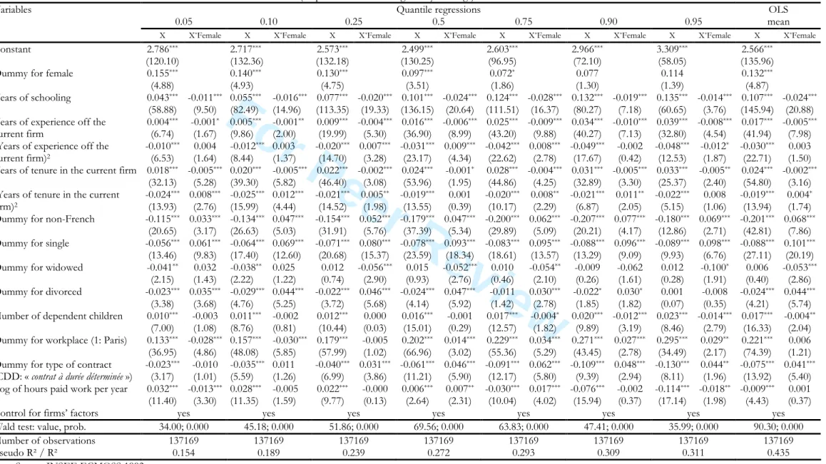
the pooled dataset are reported in Table 2 for various specifications, the full set of estimates being reported in Table 312.
Insert Table 2 about here Insert Table 3 about here
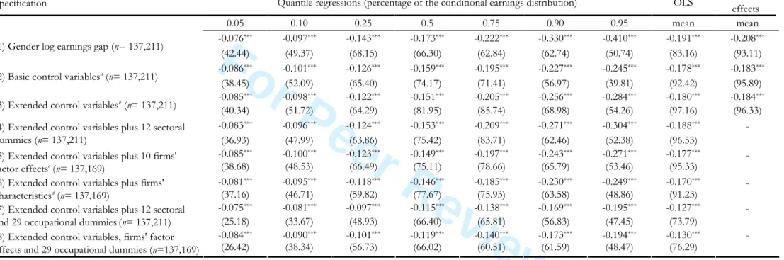
The first row presents a series of quantile regressions in which we condition the log earnings on gender at the 5th, 10th, 25th, 50th, 75th, 90th, and 95th percentiles, without any control
variable13. We notice that the observed log earnings gap increases as we move up the earnings
distribution, with a sharp acceleration after the 75th percentile. For instance, at the 75th percentile,
we see a raw gender earnings gap of slightly less than 25%. This means that the log earnings of a man at the 75th percentile of the male earnings distribution is a bit more than 22 points above the
log earnings of a woman at the 75th percentile of the female earnings distribution.
Interestingly, very similar patterns have emerged in other European countries. First, male and female earnings are closer at the bottom of the earnings distribution. Second, male and female earnings are extremely unequal at the top of the distribution, up to a maximum difference of about 50%. Third, there is a steady increase in the gender log earnings gap as we move up in the earnings distribution. Fourth, there is a sharp acceleration in the increase in the gender log earnings gap starting at about the 75th or 80th percentile in the earnings distribution. Following
Albrecht et al. (2003), De la Rica et al. (2005) or Arulampalam et al. (2004), we interpret this last feature of the gender log earnings gap by percentile as evidence of a glass ceiling.
Then, we examine various quantile estimates of the gender dummy coefficients when adding both male and female’s labour market characteristics. Several specifications have been considered, the list of explanatory variables being further described in Table 2. In what follows, we only focus on the gender dummy coefficient which indicates the extent to which the gender earnings gap remains unexplained at the different quantiles after controlling for individual differences in various combinations of characteristics. We begin by introducing into the earnings
12 In Table 3, we report the full set of estimates for the regression with firm factor effects.
3 4 5 6 7 8 9 10 11 12 13 14 15 16 17 18 19 20 21 22 23 24 25 26 27 28 29 30 31 32 33 34 35 36 37 38 39 40 41 42 43 44 45 46 47 48 49 50 51 52 53 54 55 56 57 58 59 60
For Peer Review
equations the covariates commonly used in labour economics, i.e. education, potential experience, tenure, dummies for the matrimonial status, nationality, and the number of dependent children. Then, we add job-specific variables such as the type of work contract, the workplace, the number of hours worked per year, sector of employment, and occupation.
When we control for education, experience off the current job, firm tenure, and other basic socio-economic characteristics (panel 2, Table 2), the gender dummies increase in absolute value relative to the raw gender dummy at the 5th and the 10th percentile, but then decrease from
about the 20th through the 95th percentiles. The OLS gender dummy coefficient (at the mean) also
diminishes. One explanation could be that in the first quartile of the log hourly earnings distribution, women display more labour market experience than men while this is not the case as for workers belonging to the second, third and fourth quartiles.
In the panel 3 of Table 2, we introduce the extended control variables which include basic control variables plus the type of work contract, the log of hours paid per year, and the location of the firm. The quantile estimates indicate that the gender dummy decreases in absolute value from the 5thto the median percentile as compared to the preceding model. Then, from about the
75th to the 95th, however, the gender dummy increases. This might be a first indication that
job-related characteristics (working conditions) do matter in explaining why the earnings gap is much greater at the upper tail of the earnings distribution14.
We next present the estimated gender dummy coefficients after adding 12 sectoral dummies in the quantile regressions (panel 4). The same picture emerges from these estimates, and the gender dummy is reduced only minimally at the bottom of the earnings distribution and slightly increases from about the 20th percentile and more substantially at the top of the earnings
distribution. Of course, the sector of employment is to some extent an endogenous characteristic since the choice of sector in which to work is typically made after education is completed.
13 The coefficient estimates for the gender dummy in this panel are identical to the statistical log earnings gaps.
3 4 5 6 7 8 9 10 11 12 13 14 15 16 17 18 19 20 21 22 23 24 25 26 27 28 29 30 31 32 33 34 35 36 37 38 39 40 41 42 43 44 45 46 47 48 49 50 51 52 53 54 55 56 57 58 59 60
For Peer Review
In panel 5, we account for the firms’ computed factors stemming from the factor analysis. In so doing, our aim is to substitute a firm fixed-effect regression by a “firm factor effect” regression that may account for qualitative aspects of firms’ wage policies, human capital and organisational features. In a sense, following Muller and Nordman (2004, 2005), we generalise the approach developed in Cardoso (1999) who regresses the firms’ fixed effects on different variables. For our purpose, the first ten computed factors concentrate most of the relevant information about the firms’ characteristics. A Wald test rejects at the 1 percent level the null hypothesis that the coefficients of these ten factors are jointly equal to zero. Since the covariates introduced in the factor analysis include the sectoral dummies, we omit these explanatory variables in the earnings functions.
For the sake of comparison, we have also performed a linear regression with firms’ fixed effects. The female dummy coefficient in panel 3 (-0.184) can be compared with the one estimated at the mean with the firm factor effect, which is equal to -0.177 (panel 5). So, the female coefficient is slightly reduced as we move from sector fixed effects or firm fixed effects models towards a firm factor effects specification. It may be that the computed factors stemming from our PCA of firms’ characteristics add a qualitative aspect of the firms’ wage policy to our regressions that fixed effects models, either with sector or firm dummies, may not be able to totally control for.
According to the quantile estimates reported in panel 5, we find that taking into account the firms’ factors slightly increases the gender dummy coefficient in absolute value at the lower tail of the conditional log earnings distribution (from the 5th to the median percentile).
Conversely, the coefficient is significantly reduced at the upper tail of the distribution, especially above the 75th percentile. Now, the gender earnings gap amounts to about 27% at the 95th
percentile while it amounted to more than 30% with the extended and sectoral control variables. 14 For instance, men are more likely to have a temporary work contract (CDD) than women are as we move up along
the earnings distribution: 18.2% for both men and women in the first quartile against 2.5% for men and 4.5% for women in the fourth quartile.
3 4 5 6 7 8 9 10 11 12 13 14 15 16 17 18 19 20 21 22 23 24 25 26 27 28 29 30 31 32 33 34 35 36 37 38 39 40 41 42 43 44 45 46 47 48 49 50 51 52 53 54 55 56 57 58 59 60
For Peer Review
With respect to the existing literature, our results show that controlling for firms’ characteristics is likely to have a reducing effect on the extent of the glass ceiling phenomenon, albeit moderately15.
It is of interest to compare the magnitude of the gender wage gap obtained respectively with inclusion of firms’ factors (derived from the PCA) and firms’ characteristics. If we find that the various estimates lead to very similar results, this would be the sign that the PCA method may be useful to account for the firm’s environment with a minimum number of factors, thereby avoiding potential problems of multicollinearity when multiple firm-specific variables are controlled for in wage regressions. Indeed, by definition, the main components derived from the factor analysis are poorly correlated and also have the advantage to sum up the main statistical information of the firm level variables.
According to the different estimates described in Table 2, we observe that the results from these two specifications are very similar. On the one hand, the coefficients associated with the gender dummy are increasing (in absolute value) along the conditional earnings distribution, especially at the 75th percentile and above. On the other hand, once observed firms’ characteristics
are controlled for, we note that the magnitude of the coefficient on the gender variable is slightly lower with respect to the regression with firms’ factors. At the top of the distribution, the gender earnings gap is equal to 24.9% with firms’ characteristics, 27.1% with firms’ factors, while it amounts to 30.4% with extended controls and sectoral dummies.
Finally, panels 6 and 7 of Table 2 present the quantile log earnings regression estimates adding 29 occupational dummies. We present these estimates separately because there is no clear consensus as to whether occupation (and to some extent industry) should be taken into account to assess the extent of the gender wage gap. If employers differentiate between men and women through their tendency to hire into certain occupations, then occupational assignment is an outcome of employer practices rather than an outcome of individual choice or productivity
15 Note that this result is not sensitive to the number of included firms’ factors in the earnings functions. In fact,
adding more factors (up to a total of 20) does not change significantly the estimated coefficients on the gender dummy at each considered quantile of the earnings distribution.
3 4 5 6 7 8 9 10 11 12 13 14 15 16 17 18 19 20 21 22 23 24 25 26 27 28 29 30 31 32 33 34 35 36 37 38 39 40 41 42 43 44 45 46 47 48 49 50 51 52 53 54 55 56 57 58 59 60
For Peer Review
differences16. While panel 6 presents the gender dummy coefficient of a sector fixed effect model,
panel 7 accounts for the coefficients of a firm factor effect model. Again, both sets of estimates are very close.
As might be expected, controlling for occupation considerably reduces the gender gap throughout the conditional earnings distribution. In panel 7, the unexplained gender gap falls to 8.8% at the 5th percentile and, more importantly, to 22% at the 95th percentile (compared to 9.4%
and 31.7% in panel 5). We would argue that the effect of controlling for occupation on the gender earnings gap reflects the occupational segregation that may be present in France. However, we also note that if the gender earnings gap varies significantly at the upper tail of the conditional earnings distribution from panel 1 to panel 7, it remains remarkably stable at the bottom 5th or 10th percentiles.
4.2. Quantile regressions by gender
In the previous section, we have estimated the magnitude of the gender earnings gap conditional on the characteristics of the pooled sample of male and female workers at different points of the earnings distribution, thereby implicitly assuming that the returns to those characteristics were the same at various quantiles for men and women. However, this assumption seems a priori unrealistic. We now test its relevance by introducing into the earnings functions a set of the same covariates crossed with the gender dummy. Estimates of these quantile regressions are shown in Table 4, which can be compared to pooled estimates in Table 3.
Insert Table 4 about here
We use a Wald test to assess the joint significativeness of the crossed variables all along the conditional earnings distribution. The values of the statistics at each considered percentile reveal that we have to reject the hypothesis of joint nullity of the crossed variables at the 1%
16 Conversely, one can argue that analyses that omit occupation and industry may overlook the importance of
background and choice-based characteristics on wage outcomes, while analyses that fully control for these variables may undervalue the significance of labour market constraints on wage outcomes (Altonji and Blank, 1999).
3 4 5 6 7 8 9 10 11 12 13 14 15 16 17 18 19 20 21 22 23 24 25 26 27 28 29 30 31 32 33 34 35 36 37 38 39 40 41 42 43 44 45 46 47 48 49 50 51 52 53 54 55 56 57 58 59 60
For Peer Review
level. This rejection of the pooling assumption therefore implies that gender specific equations (i.e. for men and for women) have to be estimated instead. More specifically, Table 4 is indicative of which return of the introduced labour market characteristics significantly differs across genders at each considered quantile.
We notice that almost all returns vary across the sexes whatever the workers’ relative position in the conditional distribution. This is all the more true for the returns to human capital, i.e. schooling and experience, which are always significantly lower for women. The only exception is for the return to tenure at the midpoint of the distribution (50th percentile). Interestingly, some
demographic characteristics, such as the number of dependent children or a dummy for being widowed (the reference is being married), have differentiated impacts between men and women depending on their relative position in the earnings distribution. For instance, while the wage premium for the number of children is not significantly different between men and women in the lower tail of the conditional distribution (percentiles 5th to 50th), this premium differs increasingly
across gender as we move up in the distribution.
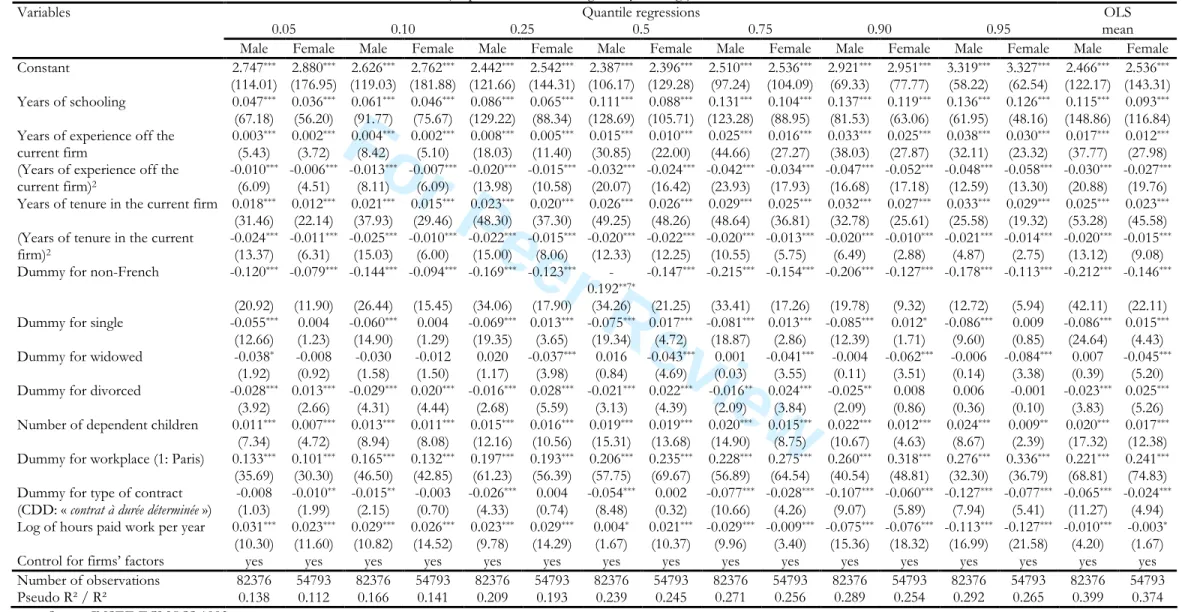
Insert Table 5 about here
Differentiated regressions by gender are then displayed in Table 5. Let us briefly describe the influence of a few explanatory variables. As previously noticed, the returns to human capital are always lower for women. For instance, the return to schooling increases, respectively for men and women, from 4.2% versus 3.3% at the 5th percentile to 13.4% versus 12.5% at the 95th
percentile. Also, while the marginal return to potential experience off the current job is decreasing for both genders (the quadratic term is negative), it diminishes more rapidly for males than for females. Other results are worth noting. First, being divorced is detrimental to men, but not to women. Second, the wage premium for working in the Paris area is higher for men in the lower tail of the distribution but, then, in the upper tail, the reverse is true: women have certainly access to better jobs there. These results provide therefore incentives to perform earnings decompositions at quantiles instead of only looking at decompositions at the sample mean.
3 4 5 6 7 8 9 10 11 12 13 14 15 16 17 18 19 20 21 22 23 24 25 26 27 28 29 30 31 32 33 34 35 36 37 38 39 40 41 42 43 44 45 46 47 48 49 50 51 52 53 54 55 56 57 58 59 60
For Peer Review
4.3. Quantile decomposition
After having analysed the extent to which returns to exogenous factors differ between men and women, we now perform a quantile decomposition of the gender gap. As in Albrecht et al. (2003) and following the recent approach described in Machado and Mata (2005), we decompose the difference between the male and female log earnings distributions into two components17. The first one is due to differences in labour market characteristics between male
and female employees. The second one is due to differences in the rewards that both men and women receive for their (observable) characteristics.
Instead of relying on the Oaxaca-Blinder decomposition technique whose purpose is to identify the sources of differences between the means of two distributions, we implement the decomposition at each quantile of the earnings distribution. Let us briefly describe the approach developed by Machado and Mata (2005). For the presentation, let m
β
and fβ
denote respectively men and women’s returns to labour market characteristics mx and f
x respectively. The decomposition of the difference between the male and female earnings densities is:
)) ( ) ( ( ) ( ) ( ) ( ) (
θ
β
θ
β
θ
β
θ
β
θ
β
m f f m f f m m f m x x x x x − = − + − (2)In the above equation, the first term on the right hand side indicates the magnitude of the gap which is due to dissimilarities in labour market characteristics. The second term indicates the magnitude of the gap which is due to differences in the rewards to these characteristics. As two counterfactual densities may be constructed, we choose to generate the density that would arise if women were endowed on the basis of men’s labour market characteristics and paid like women.
To construct the counterfactual density, we rely on the three following steps. First, we draw a sample of 150 numbers from a standard uniform distribution. Second, using these different numbers θj ( j=1,...,150), we estimate the quantile regressions coefficient vectors
17 For further discussion on decomposition methods and the gender wage gap, see Silber and Weber (1999).
3 4 5 6 7 8 9 10 11 12 13 14 15 16 17 18 19 20 21 22 23 24 25 26 27 28 29 30 31 32 33 34 35 36 37 38 39 40 41 42 43 44 45 46 47 48 49 50 51 52 53 54 55 56 57 58 59 60
For Peer Review
) ( j
f
θ
β
for the various j using the female subsample. Third, for each value of j, we take a draw with replacement from the male data set and generate the predicted wage xmβ
f(θ
j). Two additional comments are in order. First, in order to get standard errors for the counterfactual density, we have replicated the whole procedure exactly 40 times. Second, as the procedure is excessively time-consuming with very large samples, we perform the quantile decomposition on the basis of a random sample of 34 303 employees (i.e. the sample rate is 1 employee out of 4).Insert Table 6 about here
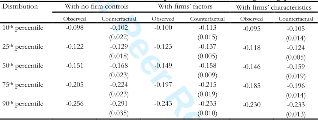
When applying the quantile decomposition, we again wonder whether the inclusion of firms’ factors or characteristics may affect the underlying conclusions. Specifically, we provide the decomposition results for three specifications, i.e. with no firms variables, with firms’ factors, and with firms’ characteristics. Results from the decompositions are given in Table 6.
In the first, third and fifth columns, we report the observed gender gaps at respectively the 10th, 25th, 50th, 75th and 90th percentile of the distribution for the various specifications. The
gender gaps reported in columns 2, 4 and 6 are constructed using women’s returns only, and then assuming that these women have the male distribution of labour market characteristics. In any cases, we observe that the gender gap strongly increases throughout the earnings distribution. Interestingly, the gap due to differences in the returns to observable characteristics is of very similar magnitude independently on the inclusion of firm factors or firm characteristics.
Our results are in fact very similar to those obtained in Sweden by Albrecht et al. (2003). We clearly observe that gender differences in labour market characteristics do not really explain the larger gap observed at the top of the distribution. Instead, the gender gap is mainly due to the differential rewards that women receive for their own characteristics. It is clear from the results of Table 6 that women would receive much lower wages were they paid as women while being endowed with male characteristics. Hence, in France, our main finding is that the glass ceiling
3 4 5 6 7 8 9 10 11 12 13 14 15 16 17 18 19 20 21 22 23 24 25 26 27 28 29 30 31 32 33 34 35 36 37 38 39 40 41 42 43 44 45 46 47 48 49 50 51 52 53 54 55 56 57 58 59 60
For Peer Review
effect is mainly due to differences in returns to observed labour market characteristics across genders at the top of the distribution rather than to differences in those characteristics.
5. Discussion and concluding comments
In this paper, we have brought empirical evidence on the glass ceiling effect according to which the gender wage gap is more important at the upper tail of the wage distribution. While several studies have recently shed light on this phenomenon in European countries (Albrecht et al., 2003; De la Rica et al., 2005; Arulampalam et al., 2004), our contribution is the first one to account for both characteristics of employers and employees. It is only recently that researchers have acknowledged that the use of matched employer-employee data for studying labour market discrimination can deepen the understanding of sex segregation in the professional environment (Hellerstein and Neumark, 2005). Interestingly, while the role of the firm characteristics has been neglected so far in studies dealing with the gender gap, we believe that the work environment is likely to affect the magnitude of the gender wage gap along the earnings distribution.
Specifically, we assess the relevance of the glass ceiling hypothesis using the French 1992 ECMOSS data, which provides rich information on about 130,000 employees and 14,000 employers. Econometric results from quantile regressions show that there exists a significant glass ceiling effect in France. While male and female earnings are close at the bottom of the income distribution, there is a strong increase in the gender earnings gap above the 75th percentile of this
distribution. In order to control for the firms’ characteristics, we follow Muller and Nordman (2004, 2005) and rely on a principal component analysis to extract the most influential factors of the surveyed establishments. This approach allows accounting for qualitative aspects of the firms including their implemented wage policy, which may not be the case when one controls for unobserved heterogeneity through firm fixed effect models.
According to the French data, the gender earnings gap would be overstated at the top of the distribution if the influence of firms’ characteristics were omitted. Hence, accounting for
job-3 4 5 6 7 8 9 10 11 12 13 14 15 16 17 18 19 20 21 22 23 24 25 26 27 28 29 30 31 32 33 34 35 36 37 38 39 40 41 42 43 44 45 46 47 48 49 50 51 52 53 54 55 56 57 58 59 60
For Peer Review
related characteristics as well as for characteristics of the workers’ environment has a reducing effect on the extent of the glass ceiling phenomenon. The reduction of the observed gender wage gap once firm characteristics are controlled for may be understood in a context of sorting among firms, where productive firms primarily form relationships with productive workers. In this setting, the gender wage gap may arise as a result of sorting of male and female workers across firms that pay different wages. If this hypothesis is true, accounting for the firm characteristics should reduce the magnitude of the gender wage gap, if not clear it up totally. In other words, the gender gap may be non-existent within firms if the gender pay gap is only linked to sorting. However, this does not provide any convincing argument as for the persistence of larger wage gaps at the upper tail of the wage distribution.
Other forces that would rationalize the existence of the glass ceiling effect may also be at work. Despite of the reduction in the earnings gap for the most paid workers, there is still a large and significant difference between the male and female earnings. Furthermore, our counterfactual decomposition shows that the glass ceiling effect is mostly due to differences in the returns to labour market characteristics across genders at the top of the distribution rather than to average differences in these characteristics. Hence, our results are very similar to those reported in recent studies conducted in Europe. As there is now robust evidence on the magnitude of the glass ceiling effect in industrialised countries, it would be worthwhile to deepen the understanding of the origins and causes of this stylised fact. We leave this issue for future research.
3 4 5 6 7 8 9 10 11 12 13 14 15 16 17 18 19 20 21 22 23 24 25 26 27 28 29 30 31 32 33 34 35 36 37 38 39 40 41 42 43 44 45 46 47 48 49 50 51 52 53 54 55 56 57 58 59 60
For Peer Review
References
Abowd, J.M. and Kramarz, F. (1999) The analysis of labor markets using matched employer-employee data, in Handbook of Labor Economics (Eds) O.C. Ashenfelter and D. Card, vol. 3B, Elsevier, North-Holland, pp. 2629-2710.
Abowd, J.M., Kramarz, F. and Margolis, D. N. (1999) High-wage workers and high-wage firms, Econometrica, 67, 251-333.
Abowd, J., Kramarz, F., Margolis, D.N. and Troske, K.R. (2001) The relative importance of employer and employee effects on compensation: A comparison of France and the United States, Journal of the Japanese and International Economies, 15, 419-436.
Albrecht, J., Björklund, A. and Vroman, S. (2003) Is there a glass ceiling in Sweden?, Journal of Labor Economics, 21, 145-177.
Albrecht, J., van Vuuren, A. and Vroman, S. (2006) Counterfactual distributions with sample selection adjustments: Econometric theory and an application to the Netherlands, mimeo, University of Georgetown.
Altonji, J.G. and Blank, R.M. (1999) Race and gender in the labor market, in Handbook of Labor Economics (Eds) O.C. Ashenfelter and D. Card, vol. 3C, Elsevier, North-Holland, pp. 3143-3258.
Arulampalam, W., Booth, A.L. and Bryan, M.L. (2004) Is there a glass ceiling over Europe? Exploring the gender pay gap across the wages distribution, mimeo, University of Auckland. Bayard, K., Hellerstein, J., Neumark, D. and Troske, K. (2003) New evidence on sex segregation
and sex differences in wages from matched employer-employee data, Journal of Labor Economics, 21, 887-922.
Blau, F. and Kahn, L. (2000) Gender differences in pay, Journal of Economic Perspectives, 14, 75-99. Booth, A., Francesconi, M. and Frank, J. (2003) A sticky floors model of promotion, pay and
gender, European Economic Review, 47, 295-322.
Buchinsky, M. (1998) Recent advances in quantile regression models: A practical guideline for empirical research, Journal of Human Resources, 33, 88-126.
Cardoso, A. R. (1999) Firms’ wage policies and the rise in labor market inequality: The case of Portugal, Industrial and Labor Relations Review, 53, 87-102.
Caroli, E., Greenan, N. and Guellec, D. (2001) Organizational change and skill accumulation, Industrial and Corporate Change, 10, 481-506.
De la Rica, S., Dolado, J.J. and Llorens, S. (2005) Ceiling and floors: Gender wage gaps by education in Spain, IZA Discussion Paper, n° 1483.
Destré, G. (2003) Fonctions de gains et diffusion du savoir : une estimation sur données françaises appariées, Economie et Prévision, 158, 89-104.
Destré, G. and Nordman, C. (2002) The impacts of informal training on earnings: Evidence from French, Moroccan and Tunisian employer-employee matched data, L’Actualité Économique, 78, 179-205.
Greenan, N. (2003), Organisational change, technology, employment and skills: An empirical study of French manufacturing, Cambridge Journal of Economics, 27, 287-317.
Hahn, J. (1995) Bootstrapping quantile regression estimators, Econometric Theory, 11, 105-121.
3 4 5 6 7 8 9 10 11 12 13 14 15 16 17 18 19 20 21 22 23 24 25 26 27 28 29 30 31 32 33 34 35 36 37 38 39 40 41 42 43 44 45 46 47 48 49 50 51 52 53 54 55 56 57 58 59 60
For Peer Review
Hellerstein, J. and Neumark, D. (2005) Using matched employer-employee data to study labor market discrimination, IZA Discussion Paper, n°1555.
Hinks, T. (2002) Gender wage differentials and discrimination in the New South Africa, Applied Economics, 34, 2043-2052.
Ichino, A. and Filippin, A. (2005) Gender wage gap in expectations and realizations, Labour Economics, 12, 125-145.
Jellal, M., Nordman, C. and Wolff, F-C. (2005) Gender wage gap under uncertainty, mimeo, DIAL, Paris.
Koenker, R. (2005) Quantile Regression, Econometric Society Monograph Series, Cambridge University Press.
Koenker, R. and Bassett, G. (1978) Regression quantiles, Econometrica, 46, 33-50.
Lindbeck, A. and Snower, D.J. (2000) Multitask learning and the reorganization of work: From tayloristic to holistic organization, Journal of Labor Economics, 18, 353-376.
Machado, J.A. and Mata, J. (2005) Counterfactual decomposition of changes in wage distributions using quantile regression, Journal of Applied Econometrics, 20, 445-465.
Meng, X. (2004) Gender earnings gap: The role of firm specific effects, Labour Economics, 11, 555-573.
Meng, X. and Meurs, D. (2004) The gender earnings gap: Effects of institutions and firms – A comparative study of French and Australian private firms, Oxford Economic Papers, 56, 189-208.
Muller, C. and Nordman, C. (2004) Which human capital matters for rich and poor’s wages? Evidence from matched worker-firm data from Tunisia, mimeo, CREDIT Research Paper 04/08, University of Nottingham.
Muller, C. and Nordman, C. (2005) Firm effects or firm human capital? An investigation of wages from French matched worker-firm data, mimeo, University of Alicante.
Nielsen, H. S. (2000) Wage discrimination in Zambia: An extension of the Oaxaca-Blinder decomposition, Applied Economics Letters, 7, 405-408.
Sakellariou, C. (2004) The use of quantile regressions in estimating gender wage differentials: A case study of the Philippines, Applied Economics, 34, 1001-1007.
Silber, J. and Weber, M. (1999) Labour market discrimination: Are there significant differences between the various decomposition procedures?, Applied Economics, 31, 359-365.
3 4 5 6 7 8 9 10 11 12 13 14 15 16 17 18 19 20 21 22 23 24 25 26 27 28 29 30 31 32 33 34 35 36 37 38 39 40 41 42 43 44 45 46 47 48 49 50 51 52 53 54 55 56 57 58 59 60
For Peer Review
Table 1. Description of the workers’ characteristicsMain sample characteristics Mean [Min ; Max ] Standard dev.
Number of observed employees per establishment 18.99 [2 ; 152] 15.53
Sex (1 for men, 0 otherwise) 0.60
Age 37.68 [16.25 ; 65] 10.30
Nationality (1 if French, 0 otherwise) 0.93
Hourly earnings (gross wage plus payments in kind, all
divided by the number of paid hours over the year) 69.48 [29.00 ;395.83] 39.49
Education (number of completed years of schooling) 12.77 [8 ; 18] 1.65
Potential previous experience (Number of years of
labour market experience: age - tenure - education – 6) 9.27 [0 ; 48.91] 8.72
Tenure in the current establishment (number of years of
tenure) 9.71 [0 ; 46.5] 8.84
Executives (1 if executive, 0 otherwise) 0.11
Number of hours paid work per year 1671.78 [33 ; 2310] 585.46
Type of contract (1 if fixed duration contract, 0
otherwise) 0.08
Workplace (1 if Paris, 0 otherwise) 0.19
Survey INSEE ECMOSS 1992.
The size of the sample is 137 211 employees, working in 14 693 establishments.
3 4 5 6 7 8 9 10 11 12 13 14 15 16 17 18 19 20 21 22 23 24 25 26 27 28 29 30 31 32 33 34 35 36 37 38 39 40 41 42 43 44 45 46 47 48 49 50 51 52 53 54 55 56 57 58 59 60
For Peer Review
26
Table 2. Gender dummy coefficients using alternative quantile earnings models (Dependent variable: log hourly earnings)
Specification Quantile regressions (percentage of the conditional earnings distribution) OLS Firm fixed
effects
0.05 0.10 0.25 0.5 0.75 0.90 0.95 mean mean
-0.076*** -0.097*** -0.143*** -0.173*** -0.222*** -0.330*** -0.410*** -0.191*** -0.208***
(1) Gender log earnings gap (n= 137,211)
(42.44) (49.37) (68.15) (66.30) (62.84) (62.74) (50.74) (83.16) (93.11)
-0.086*** -0.101*** -0.126*** -0.159*** -0.195*** -0.227*** -0.245*** -0.178*** -0.183***
(2) Basic control variablesa
(n= 137,211)
(38.45) (52.09) (65.40) (74.17) (71.41) (56.97) (39.81) (92.42) (95.89)
-0.085*** -0.098*** -0.122*** -0.151*** -0.205*** -0.256*** -0.284*** -0.180*** -0.184***
(3) Extended control variablesb
(n= 137,211) (40.34) (51.72) (64.29) (81.95) (85.74) (68.98) (54.26) (97.16) (96.33)
-0.083*** -0.096*** -0.124*** -0.153*** -0.209*** -0.271*** -0.304*** -0.188*** -
(4) Extended control variables plus 12 sectoral
dummies (n= 137,211) (36.93) (47.99) (63.86) (75.42) (83.71) (62.46) (52.38) (96.53)
-0.085*** -0.100*** -0.123*** -0.149*** -0.197*** -0.243*** -0.271*** -0.177*** -
(5) Extended control variables plus 10 firms' factor effectsc
(n= 137,169) (38.68) (48.53) (66.49) (75.11) (78.66) (65.79) (53.46) (95.33)
-0.081*** -0.095*** -0.118*** -0.146*** -0.185*** -0.230*** -0.249*** -0.170*** -
(6) Extended control variables plus firms' characteristicsd
(n= 137,169) (37.16) (46.71) (59.82) (77.67) (75.93) (63.58) (48.86) (91.23)
-0.075*** -0.081*** -0.097*** -0.115*** -0.138*** -0.169*** -0.195*** -0.127*** -
(7) Extended control variables plus 12 sectoral
and 29 occupational dummies(n= 137,211) (25.18) (33.67) (48.93) (66.40) (65.81) (56.83) (47.45) (73.79)
-0.084*** -0.090*** -0.101*** -0.119*** -0.140*** -0.173*** -0.194*** -0.130*** -
(8) Extended control variables, firms' factor
effects and 29 occupational dummies (n=137,169) (26.42) (38.34) (56.73) (66.02) (60.51) (61.59) (48.47) (76.29)
Survey INSEE ECMOSS 1992.
Absolute values of t statistics are in parentheses. ***, ** and * mean respectively significant at the 1%, 5% and 10% levels.
a: basic control variables include education, experience off the current job, tenure in the current firm, their squared values, a dummy for non-French workers, dummies for the matrimonial status (single, widowed, divorced) and the number of dependent children.
b: extended control variables include the basic control variables mentioned above plus a dummy for the workplace (1 if Paris region), a dummy for the type of work contract (1 if CDD, “Contrat à durée déterminée”) and the logarithm of the number of hours paid work per year.
c: the variables introduced in the factor analysis are a4, a44, s1, s2, s3, s4, s5, s6, s7, s8, s9, s10, s11, s12, ff1, ff2, ff3, ff4, va1, va2, va3, d21, d31, d32, d4a1, d4b1, d4b2, ps1, d151, d19a1, d19b1, d19b2, d19b3, d250, d251, d252, d253, d26a1, d26b1, d281, d301, d311, d321, d331, d332, d333, d341, d342, d3513, d3523, d3533, d3543, d3553, d3563, d3573, d3583, d3911, d3921, d39b1, d411.
d: the firm characteristics introduced in the regressions are S1, S2, S3, S4, S5, S6, S7, S8, S9, S10, S11, T2, T3, T4, T5, T6, FF2, FF3, FF4, VA1, VA2, D21, D32, D4A1, D4B1, D4B2, PS1, D151, D19B1, D19B2, D19B3, D252, D253, D26A1, D26B1, D281, D301, D311, D321, D331, D332, D341, D342, D331, D332, D3513, D3523, D3533, D3543, D3553, D3563, D3573, D3583, D39B1, D411.
Editorial Office, Dept of Economics, Warwick University, Coventry CV4 7AL, UK
3 4 5 6 7 8 9 10 11 12 13 14 15 16 17 18 19 20 21 22 23 24 25 26 27 28 29 30 31 32 33 34 35 36 37 38 39 40 41 42 43 44 45 46 47 48 49 50 51 52 53 54 55 56 57