From DSL to HPC Component-Based Runtime: A Multi-Stencil DSL Case Study

HAL Id: hal-01215992

https://hal.inria.fr/hal-01215992

Submitted on 16 Aug 2016

HAL is a multi-disciplinary open access

archive for the deposit and dissemination of

sci-entific research documents, whether they are

pub-lished or not. The documents may come from

teaching and research institutions in France or

abroad, or from public or private research centers.

L’archive ouverte pluridisciplinaire HAL, est

destinée au dépôt et à la diffusion de documents

scientifiques de niveau recherche, publiés ou non,

émanant des établissements d’enseignement et de

recherche français ou étrangers, des laboratoires

publics ou privés.

From DSL to HPC Component-Based Runtime: A

Multi-Stencil DSL Case Study

Julien Bigot, Hélène Coullon, Christian Pérez

To cite this version:

Julien Bigot, Hélène Coullon, Christian Pérez. From DSL to HPC Component-Based Runtime: A

Multi-Stencil DSL Case Study. WOLFHPC 2015 (Fifth International Workshop on Domain-Specific

Languages and High-Level Frameworks for High Performance Computing), Nov 2015, co-located with

SC’15, Austin, Texas, United States. pp.10, �10.1145/2830018.2830020�. �hal-01215992�

From DSL to HPC Component-Based Runtime:

A Multi-Stencil DSL Case Study

Julien Bigot

CEA, Maison de la Simulation USR 3441, CEA Saclay 91191 Gif-sur-Yvette, France

[email protected]

Hélène Coullon

INRIA, LIP

ENS Lyon, 46 Allée d’Italie Lyon, France

[email protected]

Christian Pérez

INRIA, LIP

ENS Lyon, 46 Allée d’Italie Lyon, France

[email protected]

ABSTRACT

High performance architectures evolve continuously to be more powerful. Such architectures also usually become more difficult to use efficiently. As a scientist is not a low level and high performance programming expert, Domain Specific Languages (DSLs) are a promising solution to automatically and efficiently write high performance codes. However, if DSLs ease programming for scientists, maintainability and portability issues are transferred from scientists to DSL de-signers. This paper deals with an approach to improve main-tainability and programming productivity of DSLs through the generation of a component-based parallel runtime. To study it, the paper presents a DSL for multi-stencil pro-grams, that is evaluated on a real-case of shallow water equations.

1.

INTRODUCTION

Programming complex scientific applications on high per-formance architectures, such as clusters of multi-core nodes containing accelerators, requires for a scientist to be an ex-pert in his own domain, but also in low level parallel and high performance programming. It can take months to years for a scientist to learn HPC programming, as it is not his main activity. As hardware continue to evolve to become more powerful but also usually more complex and difficult to use efficiently, the learning is never over.

Domain Specific Languages (DSLs) are a promising solution to hide intricate details of HPC programming from non ex-perts. By being specific to a well-defined set of problems, those languages enable the generation of well parallelized and optimized code for various architectures while requiring only a limited amount of information from the developer; part of the knowledge is directly embedded in the compiler. A critical question however concerns the specificity of DSLs. Actually, the less specific the DSL is, the more information its users must provide, and the less automatic optimizations can be embedded in the compiler. Conversely, the more spe-cific the DSL is, the less applications can use it, and the more

difficult it is to amortize the implementation cost of the DSL (language, compiler, and runtime). Programming complex-ity, as well as non-maintainability and non-portability often seem to be simply transferred from scientists to DSL design-ers.

For this reason, solutions to ease the design and implementa-tion of DSLs have recently appeared [11]. The main idea of those solutions is to propose a single DSL or a framework to write new DSLs. In this paper, we study a first contribution to another approach to improve maintainability and porta-bility in DSLs. This approach proposes a transformation from a DSL to a component-based runtime. Component-based Software Engineering has proved many times good properties for code re-use, separation of concerns, maintain-ability and productivity of codes. For this reason, we think that combining DSLs and component-based runtimes could enable those properties, by inheritance, in DSLs. This paper proposes a first evaluation of this approach though a use-case study that is a DSL for multi-stencil programs, i.e., a subclass of numerically solved partial differential equations (PDEs), and its compiler.

Many solutions to automatically optimize and parallelize nu-merical simulations have been proposed in the literature, ei-ther as specific frameworks [3, 8] or as DSLs [7, 10, 14, 23]. Most of the time, DSLs focus on the parallelization and the optimization of a single numerical computation, also called a stencil kernel. However, a real case numerical simulation (such as fluid dynamics, magneto-hydrodynamics, molecular dynamics etc.) is most of the time not composed of a single stencil kernel, but of a set of stencil kernels and a set of addi-tional local auxiliary computations [18]. The DSL proposed in this paper, called Multi-Stencil Language or MSL, is a DSL to generate a parallel component-based structure of a numerical simulation, that we call a multi-stencil program. As discussed in the related work, this work is complemen-tary to the optimization and parallelization of a single stencil kernel and is independent from implementation choices (as for example the form of the studied mesh).

The rest of this paper is organized as follows. The con-cepts of stencil kernels and multi-stencil programs are for-malized in Section 2. Section 3 gives an overview of the proposed solution while Section 4 details the MSL language and its compiler which automatically generates the parallel computation part. Section 5 introduces component mod-els and describes the proposed component-based runtime of

MSL. Section 6 focuses on a real-case simulation, solving the Shallow-water equations, and analyzes preliminary per-formance and usability results. Sections 7 states on related work, while Section 8 concludes the paper.

2.

STENCIL AND MULTI-STENCIL

2.1

Stencil Kernels

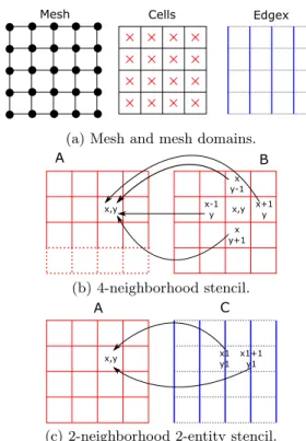
To numerically solve a set of PDEs, iterative methods (fi-nite difference, fi(fi-nite volume, fi(fi-nite element methods etc.) are frequently used to approximate the solution through a discretized (step by step) process. Thus, the continuous time and space domains are discretized so that a set of numer-ical computations are iteratively (time discretization) ap-plied onto a mesh (space discretization). In other words, in a mesh-based numerical simulation, the PDEs are trans-formed to a set of numerical computations applied at each time step on elements of the discretized space domain (the mesh). This paper focuses on one specific category of such numerical schemes based on stencil kernels [23], also called in applied mathematics explicit numerical schemes. This section introduces some definitions related to stencil kernels. A mesh is the discretization of a physical domain. It is a connected undirected graph without bridges (an edge is a bridge if its removal results in two disconnected graphs), where nodes and edges are linked to form cells (closure). Most of the time, nodes of a mesh are linked to coordinates in the real space domain. An example of structured mesh is illustrated in Figure 1a. Each cell contains four nodes and four edges. Mesh entities are elements of the mesh, such as the center of cells, edges or nodes. In Figure 1a, two mesh entities are illustrated, the center of the cells (named Cells, in red) and edges on the horizontal axis (named Edgex, in blue on left and right of each cell). A data is a simulated quantity on which computations are performed. Each data is mapped onto mesh entities. For example, in Figure 1b, data A and B are mapped onto the center of cells, while, in Figure 1c, C is mapped onto the edges.

A stencil kernel computes the value of one data or a sub-part of it (the kernel computation domain) using a numerical expression which takes as input one or more data. For ex-ample, the stencil kernel illustrated in Figure 1b computes A using B, while the one in Figure 1c computes A using C. Thus, a stencil kernel is defined by its numerical expres-sion, a set of input data (only one in the examples), and its unique output data, the result. The computation domain is a subset of the mesh entities on which the output data is mapped. For example, in the first stencil, the compu-tation of A is performed on elements represented with full lines, while dotted elements are not computed. On the other hand, on the second computation, the computation domain of A contains all the mesh entities on which it is mapped. This computation domain defines the elements over which the space loop iterates.

The numerical expression of a stencil kernel has the partic-ularity to compute each element of the result independently using some elements of the inputs in a given neighborhood. Accessed elements form a neighborhood of the output known as the stencil shape. For example, the stencil shape of the first computation in Figure 1b contains direct neighbors on the right, left, top and bottom. Sometimes, the

neighbor-Mesh Cells Edgex

(a) Mesh and mesh domains.

x,y x,y x y+1 x y-1 x-1 y x+1 y A B (b) 4-neighborhood stencil. x,y x1 y1 x1+1 y1 A C

(c) 2-neighborhood 2-entity stencil.

Figure 1: (a) a Cartesian mesh and two kind of mesh entities, (b) an example of stencil kernel on cells, (c) an example of stencil kernel on two different entities of the mesh.

hood can also access different mesh entities, as for example in Figure 1c. Actually, in this computation, the neighbor-hood contains edges on the left and on the right of a cell. As an example, the numerical expression of the first example could be:

A(x, y) = B(x + 1, y) + B(x − 1, y) + B(x, y + 1) + B(x, y − 1), and the numerical expression of the second kernel could be:

A(x, y) = A(x, y) + C(x1, y1) + C(x1 + 1, y1).

As it can be seen from these definitions, stencil kernels im-plementations share many properties from an algorithmic point of view that can be used to apply well known opti-mization and parallelization strategies. Many solutions (lan-guages or frameworks) thus propose to ease their program-ming by producing optimized and parallelized code from a simple description of the local computation to apply on each element. These are further discussed in Sections 7.

While stencil kernels have been studied a lot, the formal-ization of real overall mesh-based numerical simulations is poorly studied and not exactly for the same kind of appi-cation [18]. Actually, paying attention to complex numeri-cal simulations, it appears that most of them are composed of more than one stencil kernel, with one or more stencil shapes and of additional local computations. For example, we would like to formalize and parallelize a numerical simu-lation which chains the stencil kernels of Figures 1b and 1c. The next section formalizes concepts of stencil kernel, local kernel and multi-stencil program.

2.2

A Multi-Stencil Formalization

This section introduces some formal definitions used in the rest of the paper. Let ∆ be the set of data of the simulation A stencil kernel s is defined as the quadruplet:

s(R, w, exp, d), (1) where R is a set of pairs (r, n), with r ∈ ∆ a data read by the computation, and n the stencil shape (neighborhood) used to access r. The data written by the kernel is denoted w ∈ ∆. exp is the numerical expression of the stencil kernel. Finally the numerical expression is applied on the computa-tion domain d.

For example, in Figure 1b, assuming the computation do-main (full lines) is dc1 and the stencil shape is n1, the stencil kernel can be defined as:

R : {(B, n1)}, w : A, d : dc1,

exp : A(x, y) = B(x+1, y)+B(x−1, y)+B(x, y+1)+B(x, y−1). On the other hand, in the example of Figure 1c, assuming the computation domain is dc2 and the stencil shape is n2, the stencil kernel is defined as:

R : {(C, n2), (A, local)}, w : A, d : dc2, exp : A(x, y) = A(x, y) + C(x1, y1) + C(x1 + 1, y1). One can notice that the input data A is associated to the stencil shape local. This means that the stencil shape ap-plied on A is limited to the element with the exact same coordinate as the result element.

The specificities of kernels whose stencil shapes are all local makes it possible to apply specific optimizations. We there-fore provide a specific definition in this case. A local (or auxiliary) kernel l is defined as the quadruplet:

l(Rl, w, exp, d), (2)

where Rlis the set of input data locally accessed, and other

parameters are the same as for normal stencil kernels. We define a multi-stencil program as a sextuplet:

MSP(T, M, E, D, ∆, Γ), (3) where T is the set of time iteration to run the simulation, M is the mesh of the simulation, E is the set of mesh entities, D is the set of computation domains used for computations, ∆ is the set of data of the simulation, each one mapped onto a mesh entity, and finally Γ is the set of computations. The set of computations Γ is an ordered list of stencil and local kernels. One can notice that this work, for now, is limited to a single mesh type for a given simulation.

3.

MSL AND MSCAC OVERVIEW

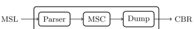
The solution proposed in this paper is based on both a do-main specific language to describe a multi-stencil program, i.e., a complete numerical simulation, and on a compiler which parses the language, applies transformations for au-tomatic parallelization, and dumps the representation to a component-based runtime, ready-to-fill with the user code. The proposed DSL, named MSL (Multi-Stencil Language), is an agnostic descriptive language for multi-stencil simula-tions. Agnostic means that the description of a numerical

MSL Parser MSC Dump CBR MSCAC

Figure 2: The three phases of the MSCAC compiler: i) the parser of the MSL description; ii) the MSC parallelization; iii) the dump to the Component-Based Runtime (CBR).

simulation does not depend on implementation choices as, for example, the type of mesh (structured or unstructured), or its associated interfaces (how to define a stencil shape, etc.). Descriptive, on the other hand, means that MSL is not made to handle the expression of numerical computa-tions, but only the description of a multi-stencil simulation, in a coarse-grain fashion. A MSL description is made of six main sections that match the six tuples elements of the definition of a multi-stencil program of Equation 3. As illustrated in Figure 2, the compiler, named MSCAC for Multi-Stencil Component Assembly Compiler, is composed of three different phases. The first phase parses the MSL description into an intermediate representation (IR). The second phase called MSC transforms the computation part (Γ) of the IR into a series-parallel tree decomposition [24] to introduce parallelism in the overall numerical simulation. Finally, the third phase dumps the IR to an actual imple-mentation of the parallel pattern of the simulation. The parallelization techniques handled by MSC are data par-allelism, where data is split among processors or cores while applying the same computation on every piece of data, and task parallelism where the program is transformed into a graph of tasks with dependencies. Different strategies can be used to schedule the tasks of this graph, i.e., to plan their execution in a valid order. The MSC compiler presented in this paper handles the transformation of the dependency graph to a static scheduling.

The final phase of compilation, the dump, uses the static scheduling of the tasks, created from Γ, and additional in-formation on T , M, ∆, E and D. It generates a program in the back-end language which embeds the parallel pattern or skeleton of the overall simulation. Various models could be used as back-end, such as OpenMP [9] for example. How-ever this paper adopts a novel approach where the dump targets a component-based runtime. This approach makes it possible to leverage good properties of software compo-nent models such as increased code re-use, eased separation of concerns, and increased maintainability and productivity. These properties counter some known limitations of DSLs. Thanks to the software components based approach, the generated code is made of four independent parts that loosely match the elements of the multi-stencil program definition. Those are the components implementing: a) the computa-tions scheduling (Γ), b) the data structures (M and E), c) data of the simulation (∆ and D), and d) the time loop (T ). The actual implementation of the numerical expres-sions are provided by the user and used in the computations scheduling. This component-based parallel structure enables to change the technology used for each part while limiting

1 program : : = ”mesh : ” meshid 2 ”mesh e n t i t i e s : ” l i s t m e s h e n t 3 ”c o m p u t a t i o n domains : ” 4 l i s t c o m p d o m 5 ” i n d e p e n d e n t : ” 6 l i s t i n d e 7 ”d a t a : ” l i s t d a t a 8 ”t i m e : ” i t e r a t i o n 9 ” c o m p u t a t i o n s : ” l i s t c o m p 10 l i s t m e s h e n t : : = meshent l i s t m e s h e n t 11 | meshent 12 l i s t c o m p d o m : : = compdom l i s t c o m p d o m 13 | compdom 14 compdom : : = compdomid ” i n ” l i s t m e s h e n t 15 l i s t i n d e : : = i n d e l i s t i n d e 16 | i n d e

17 i n d e : : = compdomid ”and ” compdomid 18 l i s t d a t a : : = d a t a l i s t d a t a 19 | d a t a 20 d a t a : : = d a t a i d ” , ” meshent 21 i t e r a t i o n : : = num 22 l i s t c o m p : : = comp l i s t c o m p 23 | comp

24 comp : : = d a t a i d ” [ ” compdomid ”]= ” compid 25 ” ( ” l i s t d a t a r e a d ” ) ”

26 l i s t d a t a r e a d : : = d a t a r e a d l i s t d a t a r e a d 27 | d a t a r e a d

28 d a t a r e a d : : = d a t a i d ” [ ” n e i g h b o r i d ” ] ” 29 | d a t a i d

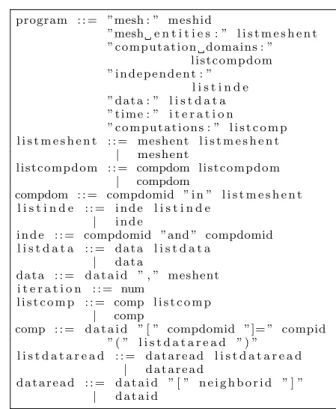
Figure 3: Grammar of the Multi-Stencil Language.

the impact on the other parts, as discussed in Section 5.

4.

LANGUAGE AND PARALLELIZATION

4.1

Multi Stencil Language

As mentioned in the previous section, the Multi Stencil Lan-guage (MSL) is an agnostic descriptive lanLan-guage for multi-stencil simulations. Six main sections are required in a MSL description that match the six elements of the formal defini-tion; they describe: 1) the mesh, 2) the mesh entities, 3) the computation domains with their inter-dependencies, 4) the data, 5) the time iterations, and finally 6) the computations. Figure 3 shows the grammar of MSL. Lines 1 to 9 define what is a MSL program with the different parts mentioned above. The remaining of this section describes these differ-ent parts of a MSL program and presdiffer-ents an example. One can notice that terminals are the string identifiers meshid, meshdom, compdomid, dataid, compid and neighborid. The terminal num is an integer terminal.

Mesh and Mesh Entities

As illustrated in the first line of the grammar in Figure 3, a mesh is simply defined by a string identifier. The different kind of mesh entities are described as a list of identifiers (Lines 2, 10 and 11 in Figure 3). Figure 4 gives an example of a mesh named cart used to represent a Cartesian mesh, and three kinds of mesh entities: cell, edgex, and edgey.

Computation Domains and Their Dependencies

A computation domain is a subset of a given kind of mesh en-tities, used for at least one computation. For each computa-tion domain, the kind of mesh entities on which it is mapped is specified (lines 3-4 and 12-14 on Figure 3). By default, two

1 mesh : c a r t 2 mesh e n t i t i e s : c e l l , edgex , e d g e y 3 c o m p u t a t i o n domains : 4 a l l c e l l in c e l l 5 a l l e d g e x in e d g e x 6 a l l e d g e y in e d g e y 7 p a r t 1 e d g e x in e d g e x 8 p a r t 2 e d g e x in e d g e x 9 i n d e p e n d e n t : 10 p a r t 1 e d g e x and p a r t 2 e d g e x 11 d a t a : 12 a , c e l l 13 b , c e l l 14 c , e d g e x 15 d , e d g e x 16 e , e d g e y 17 f , c e l l 18 g , e d g e y 19 h , e d g e x 20 i , c e l l 21 j , e d g e x 22 t i m e : 5 0 0 23 c o m p u t a t i o n s : 24 b [ a l l c e l l ]= c 0 ( a ) 25 c [ a l l e d g e x ]= c 1 ( b [ n1 ] ) 26 d [ a l l e d g e x ]= c 2 ( c ) 27 e [ a l l e d g e y ]= c 3 ( c ) 28 f [ a l l c e l l ]= c 4 ( d [ n1 ] ) 29 g [ a l l e d g e y ]= c 5 ( e ) 30 h [ a l l e d g e x ]= c 6 ( f ) 31 i [ a l l c e l l ]= c 7 ( g , h ) 32 j [ p a r t e d g e x ]= c 8 ( i [ n1 ] )

Figure 4: Example of a MSL program.

computation domains of the same entities are handled as in-tersecting except when an explicit independence relation is mentioned in the independent section of the language (lines 5-6 and 15-17 in Figure 3). On lines 4 to 6 of Figure 4, com-putation domains are defined for each kind of mesh entities: allcell, alledgex and alledgey; they are used to represent the whole domain. On lines 7 and 8, two other domains of edgex are defined: part1edgex and part2edgex; they could be used to represent the boundaries of the domain, for ex-ample, or any other sub-part of the whole domain. It is the user’s responsability to define the needed domains for his simulation. On line 10 the independence relation between part1edgex and part2edgex is specified.

Data and Time

A data element is a quantity to simulate. It is mapped on a given kind of mesh entities, as illustrated in lines 7 and 18-20 of Figure 3. The time section simply indicates a number of iterations to perform in the simulation. In the example of Figure 4 ten data elements are defined and 500 iterations (lines 11-22).

Computation Description

The last part of the language contains the specifications of stencil and local kernels as defined in Section 2.2. This de-scription does not contain a direct expression of the numer-ical expressions exp. Instead, the term exp of Equations 1 and 2 corresponds to an identifier that references an im-plementation in an external language (cf. Section 5). The description starts by the identifier of the computed data el-ement (w in the formal description) with the computation

domain between brackets (d). Then, after the equal sign, the kernel identifier (exp) is specified. Finally, between the parenthesis is the list of identifiers of the data elements read by the computation with their stencil shape between brack-ets (R). If the computation is local, no brackbrack-ets appear (Rl).

In the example of Figure 4, nine computations are described. On line 24, the data element b is computed on the domain allcell by the kernel expression c_0 which reads data a without any neighborhood shape.

4.2

MSC Parallelization

The MSC parallelization is a subpart of the overall compiler MSCAC. It makes use of the ordered list of computations Γ, which can directly be extracted from the parser, to build a parallel representation of the computations of the overall multi-stencil program. This parallelization phase is divided in five different steps to transform Γ to a series-parallel tree decomposition [24]. This sections describes these steps.

The Ordered List of Computations:

Γ is directly obtained from the parser. Actually, the list of computations in the MSL program is already ordered: Γ is a direct map of this list. In the example of Figure 4, Γ = [c0, c1, c2, c3, c4, c5, c6, c7, c8].

The Synchronized Ordered List of Computations:

Data parallelization splits data among processors and the same program is applied on each sub-part of the data. How-ever, this parallelization technique requires additional syn-chronizations between processors. The required synchro-nizations can be automatically computed from the ordered list of computations Γ. A synchronization is needed each time a data read by a stencil computation has been writ-ten by a previous computation. In such a case, a compu-tation is added before the stencil compucompu-tation. This syn-chronization computation reads the data to synchronize, and write the same data. The computation domain of such a synchronization computation encompasses the whole mesh entities on which the data is declared. As a result, Γ is transformed to a synchronized ordered list of computations Γsync. For example, in Figure 4, the stencil computation

c1 reads the data element b which has been written by c0.

For this reason the sublist [c0, c1] of Γ is transformed into

[c0, sync1, c1] in Γsync. The new computation sync1 reads

and writes b and is applied on edgex. As a result, a de-pendency is kept between c0 and sync1and between sync1,

and c1. The same transformation is performed for the two

other stencils: c4and c8. Thus, for the example of Figure 4,

Γsync= [c0, sync1, c1, c2, c3, sync4, c4, c5, c6, c7, sync8, c8].

The Dependency Graph:

From the synchronized ordered list of computations Γsync,

a dependency graph Γdepis built. A dependency exists

be-tween computations a and b (including synchronizations) if and only if a data element read by b has been written by a in Γsync with intersecting domains. Nodes of the dependency

graph represent computations of Γsync, while edges are

de-pendencies between them. The dependency graph Γdep is

a directed acyclic graph (DAG). For example, the depen-dency DAG Γdepof the example of Figure 4 is presented in

Figure 5. c0 sync1 c1 c2 c3 sync4 c5 c4 c6 c7 sync8 c8

Figure 5: Γdepof the example of Figure 4.

The Minimal Series-Parallel Graph:

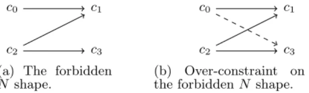
Once a dependency graph is built, many solutions can be used to build a parallel application, as for example dynamic schedulers [2, 13]. In this work a static scheduling of the dependency graph is built. To do so the dependency graph is transformed to a minimal series-parallel graph [24]. As it has been shown in [24], the transitive reduction of a DAG is a minimal series-parallel graph if and only if the forbidden shape called N-shape, illustrated in Figure 6a, is not found in the DAG. Thus, to transform Γdepto the minimal

series-parallel graph Γmsp, an algorithm is applied to remove all

N-shapes by an over-constraint [15], as illustrated in Figure 6b.

c0 c1

c2 c3

(a) The forbidden N shape.

c0 c1

c2 c3

(b) Over-constraint on the forbidden N shape. Figure 6: Forbidden N subgraph shape for a DAG to be minimal series-parallel.

The Tree Decomposition:

Many works [21, 24] explains how to build a series-parallel tree decomposition from a minimal series-parallel graph. This transformation decomposes the minimal series-parallel graph as a tree where internal nodes are sequences, indicated by a S node, and parallel sections, indicated as a P node, while leaves of the tree are the nodes of Γmsp. For example, the

series-parallel tree decomposition Γtsp of Figure 5 is

illus-trated in Figure 7.

Data parallelism optimizations:

The series-parallel tree decomposition Γtsp is used to build

the hybrid parallelization of the simulation, but it can also be used to optimize the data parallelization. In fact, it first seems natural to create the data parallel structure directly from Γsync, as the program is parallelized from data

de-composition and applying the same sequential tasks on each processor. However, as a computation kernel writes a sin-gle data w (to finely manage dependencies between tasks), the same computation domain might be iterated more than once, while some numerical expressions could be computed inside a joint space loop. For this reason, an optimized and merged ordered list of computation Γdata is built from Γtsp.

Actually, in Γtsp, computations of a parallel subtree with

a same computation domain can be computed in the same space loop, in any order. Moreover, in Γtsp, two consecutive

computations of a sequence subtree with a same computa-tion domain can be computed in the same space loop, if the computation order of the sequence is kept. For example,

S

c0 sync1 c1 P c7 sync8 c8

S S

c2 sync4 c4 c6 c3 c5

Figure 7: Γtsp of Figure 5. Nodes S represent sequences,

nodes P represent parallel sections.

from Γtsp of Figure 7, as kernels c3 and c5 are executed

in-side a parallel section, and as their computation domains are the same (alledgey), a single component K can be written peforming both computations in the same domain loop.

5.

A COMPONENT BASED BACK-END

This section describes the projection of a MSL program to a component-based runtime, including the components used to implement the static scheduling of Γtsp. The section first

gives an overview of component models, and especially the Low Level Components (L2_{C) used in this work.}

5.1

Component-Based Software Engineering

Component-based software engineering (CBSE) is a domain of software engineering [22] which promotes code re-use, sep-arations of concerns, and thus maintainability. An applica-tion is made of a set of component instances. A component is a black box that implements an independent functional-ity of the application, and which interacts with its environ-ment only through well defined interfaces: its ports. A port can, for example, specify services provided or required by the component. With respect to high performance comput-ing, some works have also shown that component models can achieve the needed level of performance, and scalability while also helping in application portability [1, 6, 19] Many component models exist, each of them with its own specificities. Well known component models include, for ex-ample, the CORBA Component Model (CCM) [17], and the Grid Component Model (GCM) [4] for distributed comput-ing, while the Common Component Architecture (CCA) [1], and Low Level Components (L2C) [5] are HPC-oriented. This work makes use of L2_{C for the experiments.}

5.2

L

_C

L2_{C [5] is a minimalist C++ based HPC-oriented}

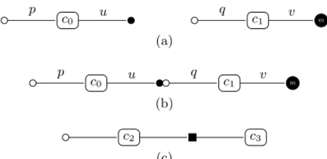
compo-nent model where a compocompo-nent extends the concept of class. The services offered by the components are specified trough provide ports, those used either by use ports for a single service instance, or use − multiple ports for multiple ser-vice instances. Serser-vices are specified as C++ interfaces. L2C also offers M P I ports that enable components to share MPI communicators. Components can also have attribute ports to be configured. As illustrated in Figures 8, a provide port is represented by a white circle, a use port with a black cir-cle, a use − multiple port by a black circle with a white m in it. MPI port are connected with a black rectangle. A L2C-based application is a static assembly of components

c0 c1 m p u q v (a) c0 c1 m p u q v (b) c2 c3 (c)

Figure 8: Example of components and their ports represen-tation. a) Component c0 has a provide port (p) and a use

port (u); Component c1 has also a provide port (q) but also

a use multiple port (v). b) A use port is connected to a (compatible) provide port. c) Component c2 and c3 shares

an MPI communicator. Driver start m T ime T Computations ∗ Γ Data ∆, D ∗ DDS M, E

Figure 9: MSCAC Component-based Runtime Overview.

instances and connections between their ports. Such an as-sembly is described in LAD, an XML dialect.

5.3

MSP Component Runtime Overview

As described in Section 3, the compiler generates four in-dependent parts in a component assembly in addition to a static part as represented in Figure 9: each rounded box rep-resents one component instance, drawn with simple lines, or more, drawn with double lines. For example, the compo-nent Data is instantiated more than once. Driver is static and drives the whole application. The four other parts are generated based on the content of the different sections of the MSL program: Computations, from the parallelization of Γ (done by MSC as explained in Section 4.2), DDS from M and E, Data from ∆ and D, and Time from T .

DDS manages the structure and the partitioning of the mesh, a single instance is generated as MSL only supports a single mesh for now. The back-end presented in this paper uses the distributed data structure proposed in SkelGIS library [8]. DDS is used by Data, for which one instance represents one data element in the MSL program. Time is parametrized by the iteration value from MSL and uses the Computations component as many times as required.

Computations contains the static scheduling Γtsp, or the

data parallel transformation Γdata, both computed by MSC.

Both transformations, Γtsp and Γdata, are encoded using

three specific components, detailed in Section 5.4, which manage the P , S, and sync operations. At the leaves of Γtsp

K * Figure 10: A kernel component K.

and Γdata, the computation components instances (denoted

K), provided by the user, are connected to Data. As shown in Figure 10, a K component provides a port to launch the computation and exposes a use port for each data element manipulated in the computation; a star is added on the use port to Data to denote it.

A complete assembly is obtained by replicating the compo-nent assembly of Figure 9 on available processors (or cores). Connections is done with MPI ports of Data components. As a result of this approach, each part of the generated code is rather independent. Changing the main time loop to use a convergence criteria rather than a fixed number of iterations would only require changing the Time component. Similarly, changing the approach used for scheduling would only im-pact the code generated in Computations. The technology used for data parallelism can also be changed by replacing the DDS and Data components, and by using the adequate interfaces in K. As a matter of fact, we have started evalu-ating an alternative based on Global Arrays [16] instead of SkelGIS.

5.4

Control Components and Dump

The series-parallel tree decomposition Γtsprepresents a static

scheduling of the simulation. Γdata, on the other hand, is

an optimized merged ordered list of computations. Both are dumped to components by generating an assembly that ex-actly matches their structure. We introduce what we call control components to represent all nodes of Γtsp or Γdata.

These components can be used for any simulation, which increases code reuse between simulations. A control compo-nent exposes a single provide port containing a control-only method, without any parameter. Three control components have been needed: SEQ, PAR, and SYNC. They are repre-sented in Figure 11.

Sequence component (SEQ) It is the direct representa-tion of a sequence node of Γtspor Γdata. This

nent sequentially calls an ordered list of other compo-nents. It exposes an ordered use-multiple port to be connected to the components to call in sequence. Parallel component (PAR) It is the direct

representa-tion of a parallel node of Γtsp (not Γdata). This

com-ponent simultaneously calls a set of other comcom-ponents. It exposes a use-multiple port to be connected to the components to call in parallel.

Synchronization component (SYNC) It is the direct rep-resentation to an update leaf of Γtsp or Γdata. This

component calls the synchronization of a given data. It exposes a use port to be connected to the data to be updated.

Then, from Γtspor Γdata, and using the control components

described above, a direct dump can be done to a component

SEQ m _{P AR} m _{SY N C}

a) Comp. SEQ b) Comp. PAR c) Comp. SYNC Figure 11: The three control components.

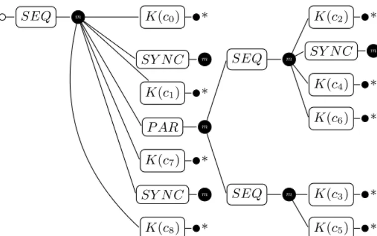
assembly for a data or hybrid (data and task) parallelization of a simulation. Figure 12 displays the assembly part corre-sponding to Γtspof Figure 7. In this figure, the ports linked

to data (use and use-multiple ports of SYNC and K) are represented but are not connected for readability. Moreover, each computation component is an instance of a specific K component using the identification name of the computation of an MSL instance. Thus, this figure represents what the component Computations of Figure 9 contains if an hybrid parallelization is performed. On the other hand, if a data parallelization is performed, a single SEQ component is used by Time, which invokes in the appropriate order the compu-tation kernels and synchronizations. Among those kernels, a single merged kernel would represent c3 and c5.

6.

REAL-CASE EVALUATION

Navier-Stokes equations is a well known set of PDEs in fluid dynamics to simulate a flow evolution in time. At the Uni-versity of Orl´eans, France, the MAPMO laboratory works on a software, called FullSWOF1, which solves the Shallow water equations obtained from the three dimensional Navier-Stokes equations, by averaging on the vertical direction [12]. Those equations are solved using a two-dimensional Carte-sian discretization of the space domain, and a finite volume numerical methods more described in [8]. We have devel-oped a MSL version of FullSWOF that contains 3 mesh entities, 7 computation domains, 48 data and 98 compu-tations. These computations are made of 32 stencil kernels and 66 local kernels.

6.1

Compiler Evaluation

The series-parallel tree decomposition Γtsp of this

simula-tion, extracted by the MSC transformasimula-tion, is composed of 17 sequence nodes and 18 parallel nodes. Figure 13 rep-resents for a given level of parallelism, i.e., the number of tasks to perform concurrently, the number of time this level is observed in the final component assembly. One can notice that the level of task parallelism extracted from the Shallow water equations is limited by two sequential parts in the ap-plication (level 1). As a level of 16 parallel tasks is reached two times, and also five times for the fourth level, sequential restrictions could be amortized. Moreover, each identified task can itself be parallelized, introducing data parallelism on loops. Thus, it is rather clear that the task parallelization technique should be used to improve the data parallelism when reaching its limits, but not to use alone. Moreover, as the level of parallelism in the application is heterogenous, the number of threads to launch for task parallelism, and the number of cores to keep for data parallelism is difficult to choose.

Figure 14 illustrates the execution time for each step of the MSC transformation for an overall execution time of ten seconds. Execution times have been computed on a laptop with a bi-core Intel Core i5 1.4 GHz, and 8 GB of DDR3.

1

SEQ m K(c₀) _* SY N C m K(c1) * P AR m SEQ m K(c2) * SY N C m K(c4) * K(c6) * SEQ m K(c₃) _* K(c5) * K(c7) * SY N C m K(c8) *

Figure 12: Component assembly representing the computation part generated from Γtsp of Figure 7.

Level 1 2 3 4 6 10 12 16 Frequency 2 1 3 5 3 1 1 2 Figure 13: Parallelism level (number of parallel tasks) and the number of times this level appears.

Step Γsync Γdep Γmsp Γtsp

Time (ms) 2 530 8297 1133 % 0.02 5.3 83.3 11.37

Figure 14: Execution times of the MSC transformation steps

One can notice that the transformation of Γdepto a minimal

series-parallel graph is the longest step of MSC, because of the removal of the forbidden N-shapes in the graph. Thus, the fact that many N-shape are removed in Γdepshows that

the creation of a static schedule of tasks may not be the best solution for complex simulations. It has to be noticed, however, that the all computation of Γtsp is still usefull to

detect how space loops can be merged in Γdata.

6.2

Preliminary Performance Evaluation

To evaluate performance of the generated component-based parallel structure, we have proceeded as follows. Our current implementation of the MSCAC compiler generates a back-end code using the SkelGIS distributed data structure as an underlying library. For this reason, our evaluation compare the shallow water equations first parallelized with a pure SkelGIS code (data structures, applicators and interfaces of SkelGIS [8]), and second parallelized with MSL (which uses the SkelGIS data structure only). Moreover, as SkelGIS library handles data parallelization for distributed memory architectures, we have limited for now our evaluations to the merged data parallelization of MSCAC (dumped from Γdata).

Evaluations have been performed on the cluster Edel of Grid’50002_{for which each node is equiped with two 8-cores}

Intel Xeon E5520, 24GB of memory, and is interconnected with an Infiniband 40G network. On Edel, three different experiments have been performed that differ in the size of

2

https://www.grid5000.fr/

the Cartesian mesh and the number of time iterations: (1) 5, 000 × 5, 000, 500 iterations; (2) 10, 000 × 10, 000, 500 it-erations; (3) 10, 000 × 10, 000, 2, 000 iterations. Figure 15 reports the results of the three experiments. The first row of graphs is the number of iterations computed per second for various number of cores. The second row of graphs repre-sents the execution time for various number of cores, using a logarithmic scale.

One can notice that, for the three different experiments, execution times of MSL, which itself uses the SkelGIS dis-tributed data structure, are improved compared to a pure SkelGIS parallelization. This result can be explained by the automatic generation of the parallel component-based run-time. Actually, in a pure SkelGIS code, communications between processes are hidden from the user through specific interfaces called applicators [8]. Using MSL, on the other hand, communications are directly managed by SY N C com-ponents, which are automatically placed in the component-based runtime by MSCAC. Thus, no overhead is introduced to hide communications. In addition to this, the scalabil-ity slope, shown by the number of iterations per second, is close to SkelGIS. This is an important result as the execu-tion time of MSL is at the same time improved compared to SkelGIS. Actually, the less the execution time is, the less the scalability capacity is. Thus, these results confirm the result of [5] that using a component-based runtime does not damage performance of the back-end code. Finally, we no-tice that SkelGIS has proved its scalability on the Shallow water equations compared to an MPI parallelization [8], that makes our performance results relevant.

7.

RELATED WORK

Many specific solutions exist to ease parallel programming of numerical simulations, as for example PATUS [7] and Pochoir [23] which propose a simple description to write stencil codes for general structured meshes, and OP2 [14] and Liszt [10] for general unstructured meshes. Those solu-tions can be considered as stencil compilers. Actually they produce optimized (cache tiling, etc.) or parallel (CUDA, OpenCL, etc.) codes for a single stencil computation. Re-cently, domain specific languages for very specific numerical methods such as ExaSlang [20] for multigrid solvers, have also been proposed.All those solutions let the user

imple-0 50 100 150 200 250 300 cores 0 2 4 6 8 10 12 14 16 18

iterations per second

Ideal MSL SkelGIS

(a) 5k × 5k mesh, 500 iterations

0 50 100 150 200 250 300 cores 0.0 0.5 1.0 1.5 2.0 2.5 3.0 3.5 4.0

iterations per second

Ideal MSL SkelGIS (b) 10k × 10k mesh, 500 iterations 0 50 100 150 200 250 300 cores 0.0 0.1 0.2 0.3 0.4 0.5 0.6 0.7 0.8 0.9

iterations per second

Ideal MSL SkelGIS (c) 10k × 10k mesh, 2k iterations 23 ₂4 ₂5 ₂6 ₂7 ₂8 log cores 25 26 27 28 29 210 211

log execution time

MSL SkelGIS (d) 5k × 5k mesh, 500 iterations 24 ₂5 ₂6 ₂7 ₂8 log cores 27 28 29 210 211 212

log execution time

MSL SkelGIS

(e) 10k × 10k mesh, 500 iterations

24 ₂5 ₂6 ₂7 ₂8 log cores 29 210 211 212 213 214

log execution time

MSL SkelGIS

(f) 10k × 10k mesh, 2k iterations Figure 15: The first line represents, for each experiment, the number of iteration computed per second for a given number of cores. The second line represents, for each experiment, the execution time for a given number of cores, using a logarithmic scale.

ment their own stencil codes in a sequential programming style, and produce high performance codes for shared mem-ory architectures and sometimes distributed memmem-ory archi-tectures. Most stencil compilers, though, handle the paral-lelization or the optimization of a single stencil kernel, con-sidering that it represents the main computation time of numerical simulations. However, most real case numerical simulation are composed of more than one stencil kernel, involving one or more stencil shapes, and additional local kernels, as explained in Section 2.2.

Other solutions, as SkelGIS library [8] or Global Arrays [16] propose more or less specialized distributed data structures (specific meshes for SkelGIS, general arrays for Global Ar-rays), which simplifies or totally hide communications and synchronizations between processes.

Halide [18] is a DSL which focusses on the automatic par-allelization and optimization of stencil pipelines in image processing. Thus, this work is the closest to MSL. How-ever, at least one important difference can be noticed: the specific domain it is applied on. Actually, image process-ing is applied onto 2D or 3D grids, while explicit numeri-cal schemes to solve PDEs can be applied on many differ-ent meshes (grids, but also unstructured or hybrid meshes). This main difference is the reason why MSL is a descriptive and agnostic language, and why it does not target specific optimizations, as tiling for example.

The work presented in this paper takes place at a different

abstraction level and can be seen as complementary to sten-cil compilers or distributed data structures. The MSCAC compiler only needs the agnostic description of the overall simulation to generate a parallel pattern of the program. This parallel pattern then needs to be filled with implemen-tation parameters and compuimplemen-tation codes. Those computa-tion codes could be generated by stencil compilers or could be written using existing distributed data structures (as SkelGIS in this paper). As a result, MSL is not a new con-tribution to stencil compilers, to tiling optimizations, or to distributed data structures, but proposes a coarse-grain au-tomatic parallelization of an overall multi-stencil program. Finally, MSL is a case study to show that component-based runtimes could improve maintainability adn flexibility of DSLs with a low impact on performance.

8.

CONCLUSION

This paper has presented the domain specific language MSL and its compiler MSCAC designed to produce a parallel (data and hybrid) component-based runtime of an overall multi-stencil program, i.e., a mesh-based numerical simula-tion reduced to explicit schemes. After details on the lan-guage and its compiler, MSL has been evaluated by the de-scription of a real case numerical simulation: the shallow water equations. The component-based data parallelization of the simulation has been compared to a pure SkelGIS par-allelization, and has shown improved execution times as well as a promising scalability. Those results demonstrate that component-based runtimes may be relevant back-end codes

for DSLs as they do not introduce performance damage. Moreover, components bring software engineering benefits such as separation of concerns, code re-use, improving main-tainability.

Although MSL is a promising case study from DSLs to component-based runtimes, many works in progress aims at improving this first contribution. First, to more clearly show the improvement of DSLs maintainability using component-based back-end, an alternative DDS component is under study, using Global Arrays [16]. In addition to this, alternatives for the Computations component, computed by MSC, are under study such as a dump to a pure OpenMP [9] code or the use of dynamic schedulers [2, 13].

9.

ACKNOWLEDGMENTS

This work has partially been supported by the PIA ELCI project of the French FSN. Experiments presented in this pa-per were carried out using the Grid’5000 testbed, supported by a scientific interest group hosted by Inria and including CNRS, RENATER and several Universities as well as other organizations (see https://www.grid5000.fr).

10.

REFERENCES

[1] B. A. Allan et al. A component architecture for high-performance scientific computing. International Journal of High Performance Computing Applications, 20(2):163–202, 2006.

[2] C. Augonnet, S. Thibault, R. Namyst, and P.-A. Wacrenier. StarPU: a unified platform for task scheduling on heterogeneous multicore architectures. Concurrency and Computation: Practice and Experience, 23(2):187–198, 2011.

[3] S. Balay, W. Gropp, L. McInnes, and B. Smith. Efficient Management of Parallelism in Object Oriented Numerical Software Libraries. In E. Arge, A. M. Bruaset, and H. P. Langtangen, editors, Modern Software Tools in Scientific Computing, pages

163–202. Birkh¨auser Press, 1997.

[4] F. Baude, D. Caromel, C. Dalmasso, M. Danelutto, V. Getov, L. Henrio, and C. P´erez. Gcm: a grid extension to fractal for autonomous distributed components. annals of telecommunications, 64(1-2):5–24, 2009.

[5] J. Bigot, Z. Hou, C. P´erez, and V. Pichon. A low level component model easing performance portability of hpc applications. Computing, 96(12):1115–1130, 2014. [6] J. Bigot and C. P´erez. Increasing reuse in component

models through genericity. In S. Edwards and G. Kulczycki, editors, Formal Foundations of Reuse and Domain Engineering, volume 5791 of Lecture Notes in Computer Science, pages 21–30. Springer Berlin Heidelberg, 2009.

[7] M. Christen, O. Schenk, and H. Burkhart. PATUS: A Code Generation and Autotuning Framework for Parallel Iterative Stencil Computations on Modern Microarchitectures. In Parallel & Distributed Processing Symposium (IPDPS), 2011 IEEE International, pages 676–687. IEEE, May 2011. [8] H. Coullon and S. Limet. The SIPSim implicit

parallelism model and the SkelGIS library. Concurrency and Computation: Practice and

Experience, 2015.

[9] L. Dagum and R. Menon. Openmp: an industry standard api for shared-memory programming. Computational Science Engineering, IEEE, 5(1):46–55, Jan 1998.

[10] Z. DeVito, N. Joubert, F. Palacios, S. Oakley, M. Medina, M. Barrientos, E. Elsen, F. Ham, A. Aiken, K. Duraisamy, E. Darve, J. Alonso, and P. Hanrahan. SC ’11, pages 9:1–9:12, New York, NY, USA, 2011. ACM.

[11] A. Fern´andez, V. Beltran, S. Mateo, T. Patejko, and E. Ayguad´e. A data flow language to develop high performance computing dsls. In Proceedings of the Fourth International Workshop on Domain-Specific Languages and High-Level Frameworks for High Performance Computing, WOLFHPC ’14, pages 11–20, Piscataway, NJ, USA, 2014. IEEE Press. [12] S. Ferrari and F. Saleri. A new two-dimensional

shallow water model including pressure effects and slow varying bottom topography. M2AN Math. Model. Numer. Anal., 38(2):211–234, 2004.

[13] T. Gautier, J. Lima, N. Maillard, and B. Raffin. Xkaapi: A runtime system for data-flow task programming on heterogeneous architectures. In Proceedings of the 2013 IEEE 27th International Symposium on Parallel and Distributed Processing, IPDPS ’13, pages 1299–1308, Washington, DC, USA, 2013. IEEE Computer Society.

[14] M. B. Giles, G. R. Mudalige, Z. Sharif, G. Markall, and P. H. Kelly. Performance Analysis of the OP2 Framework on Many-core Architectures.

SIGMETRICS Perform. Eval. Rev., 38(4):9–15, Mar. 2011.

[15] M. Mitchell. Creating minimal vertex series parallel graphs from directed acyclic graphs. In Proc. of the 2004 Australasian Symposium on Information

Visualisation, volume 35 of APVis ’04, pages 133–139, Darlinghurst, Australia, 2004. Australian Computer Society, Inc.

[16] J. Nieplocha, B. Palmer, V. Tipparaju, M. Krishnan, H. Trease, and E. Apr`a. Advances, applications and performance of the global arrays shared memory programming toolkit. Int. J. High Perform. Comput. Appl., 20(2):203–231, May 2006.

[17] Object Management Group. Corba component model 4.0 specification. Specification Version 4.0, Object Management Group, April 2006.

[18] J. Ragan-Kelley, C. Barnes, A. Adams, S. Paris, F. Durand, and S. Amarasinghe. Halide: A language and compiler for optimizing parallelism, locality, and recomputation in image processing pipelines. In Proceedings of the 34th ACM SIGPLAN Conference on Programming Language Design and

Implementation, PLDI ’13, pages 519–530, New York, NY, USA, 2013. ACM.

[19] J. Richard, V. Lanore, and C. P´erez. Towards application variability handling with component models: 3d-fft use case study. In Proc. of The 8th Workshop on UnConventional High Performance Computing (UCHPC), Vienna, Austria, Aug. 2015. To appear.

J. Teich. Exaslang: A domain-specific language for highly scalable multigrid solvers. In Proceedings of the Fourth International Workshop on Domain-Specific Languages and High-Level Frameworks for High Performance Computing, WOLFHPC ’14, pages 42–51, Piscataway, NJ, USA, 2014. IEEE Press. [21] B. Schoenmakers. A new algorithm for the recognition

of series parallel graphs. Technical report, CWI -Centrum voor Wiskunde en Informatica, 1995. [22] C. Szyperski. Component Software: Beyond

Object-Oriented Programming. Addison-Wesley Longman Publishing Co., Inc., Boston, MA, USA, 2nd edition, 2002.

[23] Y. Tang, R. Chowdhury, B. Kuszmaul, C.-K. Luk, and C. Leiserson. The pochoir stencil compiler. In

L. Fortnow and S. P. Vadhan, editors, SPAA, pages 117–128. ACM, 2011.

[24] J. Valdes, R. Tarjan, and E. Lawler. The recognition of series parallel digraphs. In Proceedings of the Eleventh Annual ACM Symposium on Theory of Computing, STOC ’79, pages 1–12, New York, NY, USA, 1979. ACM.