HAL Id: hal-00445688
https://hal.archives-ouvertes.fr/hal-00445688
Preprint submitted on 12 Feb 2010HAL is a multi-disciplinary open access
archive for the deposit and dissemination of sci-entific research documents, whether they are pub-lished or not. The documents may come from
L’archive ouverte pluridisciplinaire HAL, est destinée au dépôt et à la diffusion de documents scientifiques de niveau recherche, publiés ou non, émanant des établissements d’enseignement et de
The Vibrations Of A Beam With A Local Unilateral
Elastic Contact
H. Hazim, Neil Ferguson, B. Rousselet
To cite this version:
H. Hazim, Neil Ferguson, B. Rousselet. The Vibrations Of A Beam With A Local Unilateral Elastic Contact. 2010. �hal-00445688�
The vibration of a beam with a local unilateral elastic contact
H.Hazima,∗, N.Fergusonb,, B.Rousseleta
a
J.A.D. Laboratory U.M.R. CNRS 6621, University of Nice Sophia-Antipolis, 06108 Valrose, Nice, France.
b
Institute of Sound and Vibration Research, University Road, Highfield, Southampton S017 1BJ, UK
Abstract
The mass reduction of satellite solar arrays results in significant panel flexibility. When such structures are launched in a packed configuration there is a possible strik-ing one with another dynamically, leadstrik-ing ultimately to structural damage durstrik-ing the launch stage. To prevent this, rubber snubbers are mounted at well chosen points of the structure and they act as a one sided linear spring. A negative consequence is that the dynamics of these panels becomes nonlinear. In this paper a solar array and a snubber are simply modelled as a linear Euler-Bernoulli beam with a one sided linear spring respectively.
A numerical and an experimental study of a beam striking a one-sided spring under harmonic excitation is presented. A finite element model representation is used to solve the partial differential equations governing the structural dynamics. The models are subsequently validated and updated with experiments.
Keywords: Nonlinear vibrations, unilateral contact, modelling
∗Corresponding author. tel: +33 04 92076276
1. Introduction
The study of the nonlinear behaviour of structures with a nonlinear contact or support is a relatively new research field of interest for many structural dynamicists. It is a branch of nonlinear dynamics with a special form of nonlinearity; the system has two linear local components and the nonlinearity comes from the interaction be-tween one with the other. It is a non differentiable nonlinearity and it could be non continuous if one or two components has a strong damping coefficient. Some papers have been published to study such systems [1–3], where the focus was to study the stability using sweep tests experimentally and comparing numerical simulations, the latter computation using special packages for nonlinear simulations.
In general, non linear dynamics is a very interesting area of modern research for many reasons; the limited application of the linear theory being one of them. The complexity of the systems studied and used in the new generation of space structures and many other mechanical systems, needs a theory which can deal with the nonlin-ear behaviour encountered. Unfortunately, there is no complete theory for nonlinnonlin-ear systems such as for the linear case, but there exists many studies which could be applied for many particular cases by themselves and from a particular point of view. The interest of the authors was to study the nonlinear systems in both the frequency and the time domains, as well as the internal properties of the systems like nonlinear normal modes (NNM) which is an extension of the well known linear normal modes (LNM) (see [4–8]) .
The objectives of the current study is to simulate the dynamics of a beam under periodic excitation when it strikes a linear spring. A finite element numerical model was produced and was validated with subsequent experimental tests.
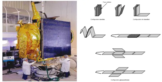
The study of the total dynamic behaviour of solar arrays in a folded position with snubbers are so complicated (see Figure 2), that to simplify, a solar array is modeled by a clamped-free Bernoulli beam with a one-sided linear spring. This system is sub-jected to a periodic excitation force. The real configuration of the problem is similar to a beam with a unilateral contact subjected to a periodic imposed displacement of the base, but the dynamical behaviour of the system does not change significantly if the imposed displacement is replaced by a periodic force excitation. The configura-tion used was easiest to be realized from a technical point of view as the experimental validation rig is very simple to build.
The experimental setup and the rig are briefly presented. The numerical results are also presented and studied in both the frequency and the time domains. It is
expected that some similarities to a linear system behaviour will be observed.
The effect of the spring location has also been studied. It is important to look for particular points to locate the spring, the aim being to reduce the nonlinear effect as much as possible. The spring was introduced at a point corresponding to the node of the second linear beam mode. In this case it is expected that the system will show a linear behaviour for an excitation near the second natural frequency; however a non-linear behaviour is expected for different excitation frequencies though. Note that no signal analysis is done by the acquisition system, as the problem is nonlinear and the standard transfer function calculation is only really applicable and useful for linear systems. The time signal was acquired and the processing performed using external software (Scilab [9]). The numerical predictions are compared to experimental results and show very good agreement.
2. Numerical modelling
The present study simulated the behaviour of a beam which strikes a snubber under a periodic excitation. As the frequency range of interest was to consider the first three linear eigen frequencies, the beam was modelled using ten linear Euler Bernoulli beam finite elements. The numerical simulations are presented and compared in the frequency domain. The Fast Fourier Transform was applied to the predicted and the experimental displacements at the free end, i.e. corresponding to the last node of the beam finite element model. The mass effect of the force transducer used for experimental validation was also taken into account in the finite element model. The beam equation of motion with an elastic snubber can be expressed as:
ρS ¨u(x, t) + EIu(iv)(x, t) = F (t)δx0 −(kru(x1, t)−)δx1 (1)
where ρ, S, E, I, F and kr are respectively the beam density, cross-sectional area,
Young’s modulus of elasticity, second moment of area, point applied harmonic force at position x0 and an elastic spring attached at position x1.
Cantilevered beam boundary conditions assume zero displacement and slope at the fixed end and zero bending moment at the free end. When the elastic unilateral spring is in contact then a shear force is present due to the reaction from the spring,
The compression of the spring is given by u(x, t)−=
(
u(x, t) if u ≤ 0
0 if u > 0 (2)
The classical Hermite cubic finite element approximation was used to solve the PDE (see [10]), it yields an ordinary nonlinear differential system in the form:
M ¨q + Kq = −[kr(qn1)−]en1 + F (t)en2 (3)
where M and K are respectively the assembled mass and stiffness matrices, q is the vector of degrees of freedom of the beam, qi = (ui, ∂xui), i = 1, ..., n, where n is the
size of M, n1 and n2 are the indices of the nodes where the spring and the excitation
force are applied to the beam respectively. Numerical time integration was performed using an ODE numerical integration for ’stiff’ problems, the package ODEPACK was used based on the BDF method (backward differentiation formula, see [9]). Small damping was introduced in the spring, there is no damping assumed in the beam structure.
3. Experimental validation
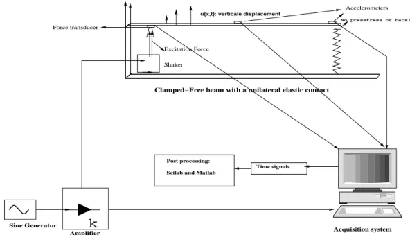
In this section, the experimental setup is briefly presented. The instrumentation used for the measurement exercises are not cited in detail as they are standard. The principal instruments used are shown in Figures 3 and 19 and include accelerometers on the beam, an electrodynamic shaker driving the beam through a force transducer and a multichannel signal analyser (Data Physics).
The physical rig consists of a cantilevered aluminum beam in contact with an elastic rubber at the free end. The beam was excited at one point with an applied periodic excitation. The beam properties and the rubber stiffness are given in Table 1. In practice, the use of a small electrodynamic shaker yields a technical problem due to the reaction of the beam. It is difficult to realize an input force F (t) which is a simple sine wave unless the impedance of the shaker is significantly higher than the beam impedance . To deal with this problem, a force transducer was fixed between the shaker and the beam to measure the actual supplied excitation force to the beam. The numerical simulations use the actual measured force signal coming from the acquisition system which was periodic. This method is an alternative to modelling the electrodynamic shaker motion. Figure 8 shows typical examples of the input force signals with the corresponding spectral content.
From a simulation and comparison shown later, using the actual measured force is appropriate given the simplified excitation system without any feedback control which would be necessary to produce a strict harmonic signal.
k
Shaker Excitation Force
u(x,t): verticale displacement
Clamped−Free beam with a unilateral elastic contact
Amplifier Sine Generator
Force transducer
Acquisition system
Post processing: Scilab and Matlab
Time signals
No presstress or backlash
Accelerometers
Figure 1. A schematic of the experimental setup.
Beam Beam Beam Beam Young’s Beam Spring
length width thickness modulus density stiffness
0.35m 0.0385m 0.003m 69 × 109N/m2 2700kg/m3 57.14 KN/m Table 1. The physical properties of the beam and the spring. The spring stiffness was evaluated using an algorithm described in (4.2).
4. Beam piecewise linear system dynamics
The system has two linear configurations or states. The first consists of the beam without the spring in contact and the second when the beam is permanently in
con-tact with the elastic support, which is modeled as a linear spring. The advantage of these two states is to give an idea on the effect of the spring on the overall system dynamics.
Usually, adding a spring to a simple beam model at one point raises the eigen fre-quency sequence for the system; this shift is realized numerically by adding the spring stiffness to the coefficient corresponding to the contact point in the stiffness matrix of the system. The spring is massless, so the mass matrix of the F.E. model is intact. Some experimental problems were encountered; one of these problems is to imple-ment a perfect clamping for the beam, which is impossible in practice but can be reasonably assumed. Another issue is that the Young’s modulus of the rubber spring used for the experiments was unknown. An algorithm was developed to determine the stiffness of the rubber for small displacements. This was subsequently used in the numerical simulations performed for comparison with experiments.
4.1. The two linear states
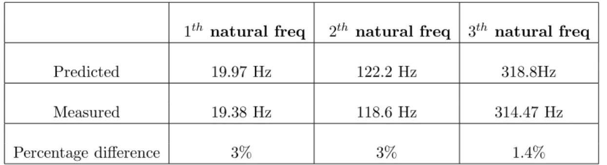
Firstly, predictions of the forced response of the cantilever beam without a point elastic support were produced and compared with the experiments. Good agreement showed that the model reasonably accurately represents the cantilever beam and its boundary conditions. The results for the natural frequencies are shown in Table 2. On the other hand, predictions of the cantilever beam with a spring permanently in contact at the free end were produced and compared with the experiments, good agreement was found (see Table 3). The last state was used to determine the stiffness of the spring using an algorithm described in the next subsection.
1th natural freq 2th natural freq 3th natural freq Predicted 19.97 Hz 122.2 Hz 318.8Hz Measured 19.38 Hz 118.6 Hz 314.47 Hz Percentage difference 3% 3% 1.4%
Table 2. The natural frequencies of the clamped-free beam
4.2. Characterization of the spring support stiffness
After initially finding the natural frequencies of the system for the two states of linearity mentioned in the pervious subsection, an algorithm was developed to find a
1th natural freq 2th natural freq 3th natural freq Predicted 84.57 Hz 246.14 Hz 443.53Hz Measured 84.47 Hz 243.5 Hz 440 Hz Percentage difference 0.1% 1% 0.7%
Table 3. The natural frequencies of the clamped beam with a permanently attached spring
suitable spring stiffness by iteration.
The shift of the frequencies due to adding a spring at the free end of the beam were recorded. The stiffness matrix of the finite element model incorporated a point spring at the node in contact. Mathematically, the problem is to find a coefficient value kr
which shifts the first eigen frequency f0 of the system without spring to f1, the first
eigen frequency of the same system with a spring permanently in contact. The method is based on the uniqueness of the sequence of the generalized eigen frequencies of the stiffness and mass matrices.
The subsequent value obtained for the point stiffness by this algorithm was krequal to
57.14KN/m. The corresponding Young’s modulus Er, assumes the stiffness krequals
to the product of the Young’s modulus with the spring area divided by the spring length. The estimated Young’s modulus for the rubber spring being 4 × 10⁶N/m2.
5. Comparison of simulations with experiments
In this section the simulations are compared to the measured data in the frequency domain; the acquisition system provides just the time signals of the accelerations and the input force. The processing of these signals and the numerical results were done using external software (Scilab [9]).
The total length of data predicted corresponds to an integration time which is fixed at t equal to 1s for all of the simulations and the acquired experiment of samples. It is five times the fundamental (lowest) period of the system. The data are measured immediately above the support and the frequency axis is normalized by the excitation frequency
three modes, hence the beam was modelled using ten equal length finite elements. In principle, the model is able to be applied to higher frequency excitations but typically any fatigue or damage in practice is likely to occur in the lower order modes.
5.1. Comparison in the frequency domain
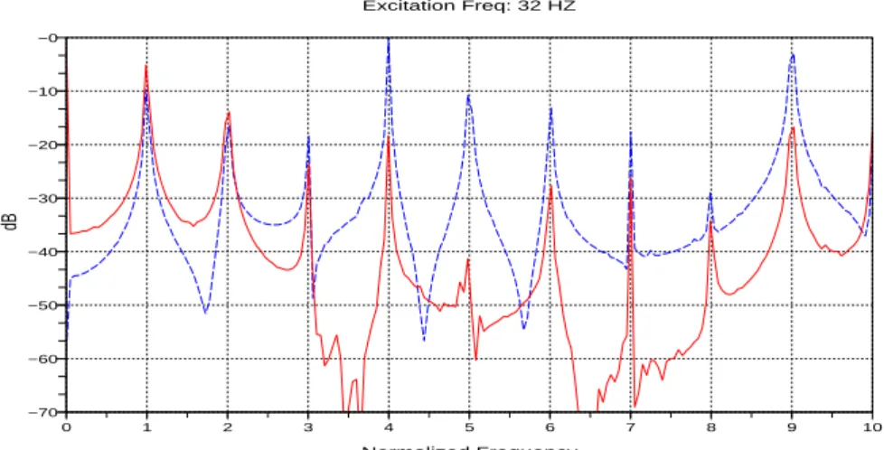
The effect of the unilateral contact is clear, the input frequency is split into its all harmonics. From an energetic point of view, the input energy is split, each subhar-monic of the main excitation takes its part thus the contribution of each harsubhar-monic is evident.
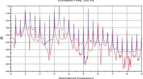
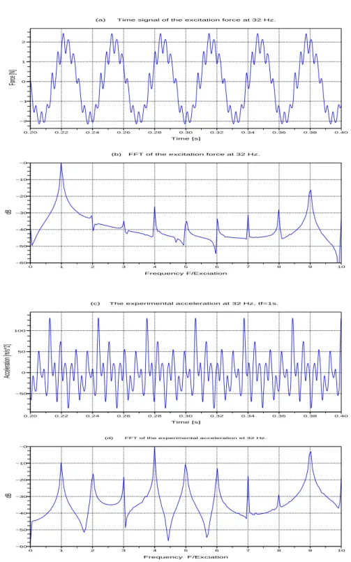
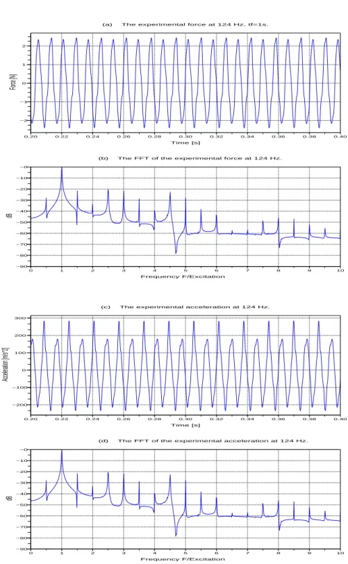
Figures 5, 6 and 7 show the FFT of the numerical and the experimental displace-ments for an excitation signal at 32 Hz, 124 Hz and 100 Hz respectively. The height of the peaks are normalized by the maximum. The predicted frequencies found are exactly the same as measured for a large number of harmonics. However, a small shift in the height of these peaks appears for the fifth harmonic; the peak in Figure 5 appears at a multiple of 5 times the original main excitation frequency, i.e. at approx-imately 160Hz in the acceleration response. At this frequency there is no guarantee that the actual support of the beam and the spring is itself rigid, as it might have its own dynamics as would the bench that supports the rig, so there might be some influence of that on the response. Other tests with random excitations have shown good agreement. Figures 8 and 9 show the input excitation force and the measured acceleration at 32 Hz and 124 Hz respectively. It is clear from the time signal and from the frequency content that the forces are not pure harmonic single frequency sine waves, but they are periodic.
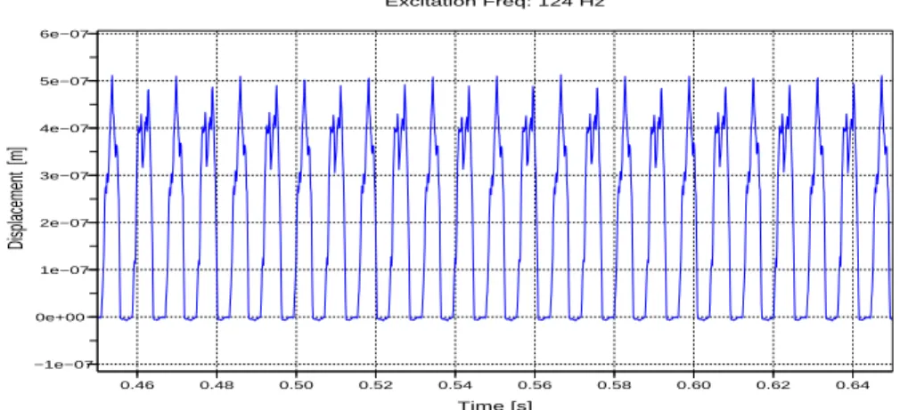
Figures 10, 11 and 12 show the predicted displacement for an excitation at 32 Hz, 124 Hz and 100 Hz respectively. The displacements are almost always positive so they have positive means. This is due to the high stiffness of the spring, but the time response is still periodic.
5.2. Magnitude-Energy dependence
The magnitude-energy dependence is a typical dynamical feature of nonlinear systems under excitation; the maximum of the solution plotted against the input energy can take different shapes depending on the form of the nonlinearity. For linear systems under periodic excitation, the maximum of the solution is proportional to the input energy. The model studied in this paper is a piecewise linear system, the numerical and the experimental results is expected to exhibit a linear behaviour for different levels of input energy.
mathematical and an experimental proof are presented to demonstrate the magnitude-energy independence. From a mathematical point of view, the level of excitation energy depends on the magnitude of the excitation force F (t). The idea here is to examine the variations of the solution in the time domain as the amplitude of the excitation force F (t) changes linearly. Consider then equation (1) and multiply both sides by a constant λ ≥ 0 the equation becomes:
λ[ρS ¨u(x, t) + EIu(iv)(x, t)] = λ[F (t)δ
x0 −(kru(x1, t)−)δx1] (4)
In general, the only problem to substitute the parameter λ in the equation is the nonlinear term; in this case, λ[kru(x1, t)−] = kr[λu(x1, t)]− (see definition of u−).
Equation (4) can then be written as follow:
ρS¨v(x, t) + EIv(iv)(x, t) = λ[F (t)δx0] − kr(v(x1, t)−)δx1 (5)
such that v = λu. In conclusion, the solution v of the PDE governing the motion is proportional to the excitation force F (t).
Note that this substitution for the parameter λ is not generally possible, e.g. if a prestress is applied between the spring and the beam; it is the case for many other nonlinearities too (λx3 6= (λx)3).
Experimentally, the mean square responses of each harmonic is plotted against the power spectral density Gxx of the input force for three levels of excitation. The mean
square response of the mode is calculated approximately by using the Mean Square Bandwidth πζωn. The experimental estimate of the equivalent viscous damping ratio
is ζ = ω2−ω1
2ωn , where ω
n is the resonance frequency, ω1 and ω2 are the frequencies
corresponding to the half-power points (-3dB below the maximum peak response). Usually, this method is used to approximate the mean square response at the natural frequency of a linear system. Herein, it is used at the first resonance frequency of the nonlinear system (32 Hz) which can be calculated as the inverse of the mean of the linear periods of the two piecewise linear systems; it is also applied to its harmonics. Figure 13 shows the mean square responses for the fundamental mode and for the first two harmonics normalized by the excitation mean square level, against three different input levels. As the excitation level increases the response at the excitation frequency and its harmonics increases proportionally, the relationship between the fundamental mode and its harmonics is linear; this linear behaviour is due to the linearity of the spring and the beam.
6. Numerical simulations
In this section, some further numerical simulations are presented in order to in-vestigate and understand better the system behaviour. Figures 14 and 15 show the
displacement for a sine excitation at 32 Hz and 124 Hz respectively; Figure 16 shows the frequency content of the displacement for a sine excitation at 32 Hz; the results cannot be compared to the experiments as it is not easy to realize a simple sine ex-citation. The dynamic behaviour of the system is similar to those presented in the previous section. The main response is split into all the subharmonics of the excita-tion frequency.
The elastic force from the spring is applied to the free end of the beam and should be taken in account as it can damage the structure; this force is non differentiable as the spring is only on contact when the beam has a negative displacement and its magnitude is proportional to the spring compression. Figure 17 and 18 show the predicted time signal of the force applied to the beam for a sine excitation at 32 Hz and 124 Hz respectively. Note that in case of a bilateral spring (spring attached to the beam), the time signal should be differentiable and periodic with a zero mean. 7. The effect of the unilateral spring position
An aim of this work is to provide a model which can predict the dynamic behaviour of a beam striking an elastic support. It is also necessary to choose the preferable points of the structure to position the support. In this section, the spring is moved to the node of the second linear beam mode which corresponds to a particular node of the F.E. model (see Figure 19). The subsequent numerical results show a linear behaviour of the system for an excitation near the second eigen frequency. They show a nonlinear behaviour as in the previous case for any other frequency of excitation. The results are presented in the frequency domain as before taking in account the new spring’s position. Figure 20 shows the FFT of the numerical and the experimental displacements for an excitation at 122 Hz, very close to the second eigen frequency of the linearized system (see Table 2). It is clear that the response primarily has a single frequency content as the input signal (Figure 21), which is a fundamental property of a linear system.
Figure 22 shows the FFT of the experimental and the numerical displacements for an excitation of 32 Hz. The input frequency is split into all subharmonics, the behaviour of the beam is the same as described in the previous section, as the system is no longer linear.
Conclusions
A numerical and experimental study of a beam with a unilateral elastic contact has been presented, the model used for the predictions having been validated by
experiments. The comparison was performed in the frequency domain for different excitation frequencies; the results showed a very good agreement.
The comparison in the time domain needs a sophisticated processing of the time do-main signals to eliminate or reduce the contribution from higher order frequencies not involved in the motion; this aspect will be in the scope of the future.
The results showed the effect of the spring position on the dynamic behaviour; other positions could be of interest if the system is subjected to high frequency excitation as the number of nodes increase with respect to the excited modes. Some experi-mental results for a pres-stressed contact is currently under investigation, this will be reported in the future. Also, future work will consider other types of excitation such as broadband random base excitation which might be present for the practical application of launching stacked solar array panels.
Acknowledgements
This work was conducted for a PhD project of the first author with a scholar-ship from Thales Alenia Space, France. The authors also gratefully acknowledge the financial support of the “Conseil G´en´erale des Alpes Maritimes” to realize this project.
References
[1] J. H. Bonsel, R. H. B. Fey, and H. Nijmeijer. Application of a dynamic vibration absorber to a piecewise linear beam system. Nonlinear Dynamics, 37:227–243, 2004.
[2] R.H.B. Fey and F.P.H. van Liempt. Sine sweep and steady-state response of a simplified solar array model with nonlinear elements. In International conference
on Structural Dynamics Modelling, pages 201 – 210, 2002.
[3] E. L. B. van de Vorst, M. F. Heertjes, D. H. van Campen, A. de Kraker, and R. H. B. Fey. Experimental and numerical analysis of the steady state behaviour of a beam system with impact. Journal of Sound and Vibration, 212(2):321 – 336, 1998.
[4] S. Bellizzi and R. Bouc. A new formulation for the existence and calculation of nonlinear normal modes. Journal of Sound and Vibration, 287(3):545 – 569, 2005.
[5] D. Jiang, C. Pierre, and S. W. Shaw. Large-amplitude non-linear normal modes of piecewise linear systems. Journal of Sound and Vibration, 272(3-5):869 – 891, 2004.
[6] G. Kerschen, M. Peeters, J.C. Golinval, and A.F. Vakakis. Nonlinear normal modes, part i: A useful framework for the structural dynamicist. Mechanical
Systems and Signal Processing, 23(1):170 – 194, 2009. Special Issue: Non-linear
Structural Dynamics.
[7] M. Peeters, R. Vigui, G. Srandour, G. Kerschen, and J.-C. Golinval. Nonlinear normal modes, part ii: Toward a practical computation using numerical contin-uation techniques. Mechanical Systems and Signal Processing, 23(1):195 – 216, 2009. Special Issue: Non-linear Structural Dynamics.
[8] S. Junca and B. Rousselet. Asymptotic expansions of vibrations with small unilateral contact. In Ultrasonic wave propagation in non homogeneous media. Springer, 2008.
[9] Scilab. A free software. Available at http://www.scilab.org/, 2009.
[10] M G´eradin. Th´eorie des vibrations: applications `a la dynamique des structures. Masson Paris, second edition, 1996.
Figure 2. Left: Solar array of a satellite under a test on a shaker. Right: A solar array from the folded to the final position
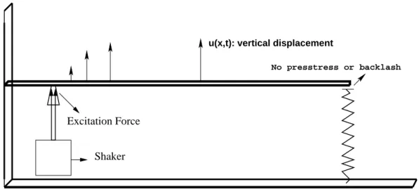
Clamped−Free beam with a unilateral elastic contact Shaker
Excitation Force
u(x,t): vertical displacement
No presstress or backlash
Figure 3. beam system with an unilateral spring under a periodic excitation
Figure 4. The rig used for the experiments: a linear clamped-free beam in contact with a rubber support (enlarged photograph on the right).
0 1 2 3 4 5 6 7 8 9 10 −70 −60 −50 −40 −30 −20 −10 −0 Excitation Freq: 32 HZ Normalized Frequency dB
Figure 5. Predicted (solid) and measured displacements (dashed) (dB) for an excita-tion at 32 Hz applied to the beam with unilateral support stiffness. The displacement is normalized by the peak value and is measured immediately above the support and the frequency axis is normalized by the excitation frequency.
0 1 2 3 4 5 6 7 8 9 10 −80 −70 −60 −50 −40 −30 −20 −10 −0 Excitation Freq:124 Hz Normalized Frequency dB
Figure 6. Predicted (solid) and measured displacements (dashed) (dB) for an excita-tion at 124 Hz applied to the beam with unilateral support stiffness. The displacement is normalized by the peak value and is measured immediately above the support and the frequency axis is normalized by the excitation frequency.
0 1 2 3 4 5 6 7 8 9 −90 −80 −70 −60 −50 −40 −30 −20 −10 −0 Excitation Freq: 100 Hz Normalized Frequency dB
Figure 7. Predicted (solid) and measured displacements (dashed) (dB) for an excita-tion at 100 Hz applied to the beam with unilateral support stiffness. The displacement is normalized by the peak value and is measured immediately above the support and the frequency axis is normalized by the excitation frequency.
0.20 0.22 0.24 0.26 0.28 0.30 0.32 0.34 0.36 0.38 0.40 −2 −1 0 1 2
(a) Time signal of the excitation force at 32 Hz.
Time [s] Force [N] 0 1 2 3 4 5 6 7 8 9 10 −60 −50 −40 −30 −20 −10 −0
(b) FFT of the excitation force at 32 Hz.
Frequency F/Exciation dB 0.20 0.22 0.24 0.26 0.28 0.30 0.32 0.34 0.36 0.38 0.40 −50 0 50 100
(c) The experimental acceleration at 32 Hz, tf=1s.
Time [s] Acceleration [m/s^2] 0 1 2 3 4 5 6 7 8 9 10 −60 −50 −40 −30 −20 −10 −0
(d) FFT of the experimental acceleration et 32 Hz.
Frequency F/Exciation
dB
Figure 8. Measured excitation force (a) and its frequency contents (b), measured acceleration response (c) and its frequency content (d) for an excitation at 32 Hz.
0.20 0.22 0.24 0.26 0.28 0.30 0.32 0.34 0.36 0.38 0.40 −2 −1 0 1 2
(a) The experimental force at 124 Hz, tf=1s.
Time [s] Force [N] 0 1 2 3 4 5 6 7 8 9 10 −90 −80 −70 −60 −50 −40 −30 −20 −10 −0
(b) The FFT of the experimental force at 124 Hz.
Frequency F/Excitation dB 0.20 0.22 0.24 0.26 0.28 0.30 0.32 0.34 0.36 0.38 0.40 −200 −100 0 100 200 300
(c) The experimental acceleration at 124 Hz.
Time [s] Acceleration [m/s^2] 0 1 2 3 4 5 6 7 8 9 10 −90 −80 −70 −60 −50 −40 −30 −20 −10 −0
(d) The FFT of the experimental acceleration at 124 Hz.
Frequency F/Excitation
dB
Figure 9. Measured excitation force (a) and its frequency contents (b), the measured acceleration response (c) and its frequency content (d) for an excitation at 124 Hz.
0.46 0.48 0.50 0.52 0.54 0.56 0.58 0.60 0.62 0.64 0e+00 1e−08 2e−08 3e−08 4e−08 5e−08 Excitation Freq: 32 Hz Time [s] Displacement [m]
Figure 10. The predicted displacements for an excitation at 32 Hz; the displacement is measured immediately above the support. The high unilateral stiffness yields almost a positive displacement. 0.46 0.48 0.50 0.52 0.54 0.56 0.58 0.60 0.62 0.64 −1e−07 0e+00 1e−07 2e−07 3e−07 4e−07 5e−07 6e−07 Excitation Freq: 124 Hz Time [s] Displacement [m]
Figure 11. The predicted displacements for an excitation at 124 Hz, the displacement is measured immediately above the support.
0.46 0.48 0.50 0.52 0.54 0.56 0.58 0.60 0.62 0.64 0.0e+00 5.0e−08 1.0e−07 1.5e−07 2.0e−07 Excitation Freq: 100 Hz Time [s] Displacement [m]
Figure 12. The predicted displacements for an excitation at 100 Hz, the displacement is measured immediately above the support.
Figure 13. The normalized mean square responses (mean square displacement divided by the mean square excitation force) in each harmonic for inputs at three different mean square force levels. The excitation frequency is 32 Hz, the acceleration is measured immediately above the support.
0.46 0.48 0.50 0.52 0.54 0.56 0.58 0.60 0.62 0.64 0.0e+00 5.0e−08 1.0e−07 1.5e−07 Excitation Freq: 32 Hz Time [s] Displacement [m]
Figure 14. The predicted displacements for a sine excitation at 32 Hz, The accelera-tion magnitude is a = 1 m/s2. The displacement is measured immediately above the
support. 0.46 0.48 0.50 0.52 0.54 0.56 0.58 0.60 0.62 0.64 0.0e+00 5.0e−08 1.0e−07 1.5e−07 2.0e−07 Excitation Freq: 124 Hz Time [s] Displacement [m]
Figure 15. The predicted displacements for a sine excitation at 124 Hz. The accel-eration magnitude is a = 1 m/s2. The displacement is measured immediately above
0 1 2 3 4 5 6 7 8 9 10 −60 −50 −40 −30 −20 −10 −0 Excitation Freq: 32 Hz Normalized Frequency dB
Figure 16. The frequency content of the predicted numerical displacement for sine excitation at 32 Hz, the displacement is measured immediately above the support. The excitation frequency is split into all its harmonics.
0.46 0.48 0.50 0.52 0.54 0.56 0.58 0.60 0.62 0.64 0 100 200 300 400 500 600 700 800
Excitation Freq: 32 Hz, a=0.1 m/s^2.
Time [s]
Force [N]
Figure 17. The predicted elastic force of the spring support for an excitation at 32 Hz. The acceleration magnitude is a = 0.1m/s2 and the spring is only in contact at
0.46 0.48 0.50 0.52 0.54 0.56 0.58 0.60 0.62 0.64 0 10 20 30 40 50
Excitation Freq: 124 Hz, a=0.1 m/s^2
Time [s]
Force [N]
Figure 18. The predicted elastic force of the spring support for an excitation at 124 Hz. The acceleration magnitude is a = 0.1m/s2 and the spring is only in contact at
times where the beam displacement is negative.
Clamped−Free beam with a unilateral elastic contact Shaker
Excitation Force
No presstress or backlash The node of the 2" mode
u(x,t): vertical displacement
Figure 20. Predicted (solid) and measured displacements (dB) for an excitation at 122 Hz applied to the beam with unilateral support stiffness. The displacement is measured immediately above the support and the frequency axis is normalized by the excitation frequency.
0.000 0.005 0.010 0.015 0.020 0.025 0.030 0.035 −1.5 −1.0 −0.5 0.0 0.5 1.0 1.5
The Force time signal. Excitation =122 HZ.
Time [s] Force [N] 0.0 0.5 1.0 1.5 2.0 2.5 3.0 3.5 −70 −60 −50 −40 −30 −20 −10 −0
Frequency F/Excitation For 122 HZ.
FFT of the Force signal [dB]
Figure 21. The time signal and its FFT of the input force for an excitation at 122 Hz.
Figure 22. Predicted (solid) and measured displacements (dB) for an excitation at 32 Hz applied to the beam with unilateral support stiffness. The displacement is measured immediately above the support and the frequency axis is normalized by the excitation frequency.