Estimates of the net excitatory currents evoked by visual stimulation of identified neurons in cat visual cortex
15
0
0
Texte intégral
(2) spike rate in neocortical neurons can be approximated by a linear system. Conventional deconvolution methods can then be used to estimate the input signal (e.g. excitatory current) from the output signal (e.g. action potential discharge) and the impulse response function (transfer response) of the neuron. It is clear, however, that all spiking neurons exhibit non-linearities; the thresholded action potential is one obvious example of this. This seems to preclude any linear systems treatment of neuronal discharge. However, recent evidence from in vitro recordings in guinea-pig visual cortex indicates that the conversion of input current to spikes can be reasonably approximated by a linear filter model with rectification (Carandini et al., 1996). Thus, there are some grounds for optimism that such linearities also might allow us to estimate the form of the excitatory current that leads to the pattern of spike discharge observed in vivo. In this paper we compare experimentally the adaptation of neurons to steps of injected current, and compare the magnitude of responses to intracellular current injections and to visual stimulation. However, the challenge is to estimate the magnitude of the time-varying net synaptic current arriving during visual stimulation. We thus used a more detailed model neuron than that used by Carandini et al. (1996) to test the acceptability of the assumption of linearity. The simulations indicated that a linear model does provide a means of achieving a useful approximation: the shape of an arbitrary input current can in fact be recovered with reasonable fidelity from the spike output. We then applied this same method to our experimental data to estimate the form and amplitude of the net somatic current during actual visual stimulation. A brief report of this work has appeared (A hmed et al. 1993).. Materials and Methods Animal Preparation The cats were prepared according to previous methods (Martin and Whitteridge, 1984; Douglas et al., 1991). Sixteen cats (1.9–4.0 kg, mean 2.5 kg) were initially anaesthetized with 2-3% Halothane in N2O/O2. The left femoral vein and artery were cannulated. Halothane was withdrawn and anaesthesia was maintained with i.v. alphaxalone–alphadolone (Saffan, Glaxo). The eyes were infiltrated with a drop of atropine sulphate (1%, w:v) and phenylepherine hydrochloride (1%, w/v) to paralyse accommodation and retract the nictitating membrane. Contact lenses of zero power were placed on the corneas and test lenses focused the eyes on a tangent screen 114 cm from the eyes. After completing the surgical procedures, Saffan anaesthesia was replaced with i.v. sodium barbiturate (loading dose 10 mg/kg, thereafter 2-3 mg/kg/h). The animal was paralysed (80 mg of gallamine triethiodide and maintained on a continuous infusion of 13 mg/kg/h with tubocurarine of 1 mg/kg/h). The animal was ventilated with a mixture of O2/N2O (30:70). End-tidal CO2 was maintained around 4.5%. The blood pressure, heart rate, EEG, end-tidal CO2 and rectal temperature were monitored continuously throughout the experiment. Classification of Neuronal Responses and Nomenclature Recordings were made in the right primary visual cortex (Horsely–Clarke AP coordinates –3 to –6 mm). Insulated tungsten stimulating electrodes were positioned in the optic chiasma (OX), in the optic radiation above the right dorsal lateral geniculate nucleus (OR1), and in the optic radiation underlying the primary visual cortex (OR2). The micropipettes were filled with 4% horseradish peroxidase (HRP) in a 0.2 M KCl solution buffered with 0.05 M Tris (pH 7.9). The impedance of the bevelled pipettes ranged between 40 and 80 MΩ. During extracellular recording neurons were functionally classified (Gilbert, 1977), their receptive fields through the right and/or left eye were mapped, and their optimal orientation and range, directional selectivity, ocular dominance class, latency to OX, OR1 and OR2 stimulation were determined (Douglas et al., 1991). Responses to visual stimuli were stored as peristimulus time. histograms (PSTHs). The DC offset and capacitance compensation were trimmed, and the electrode impedance measured before attempting intracellular impalement. Records of the intracellular potential were digitized and stored (see below). HRP was injected into the neuron using intermittent positive current pulses of between 2 and 4 nA. The responses of neurons have been classified according to the form of their action potential, or by the temporal pattern of their responses. Mountcastle et al. (1969) recording from sensorimotor cortex in vivo distinguished ‘regular’ neurons, which were encountered most frequently and had triphasic action potentials, from ‘thin spike’ neurons, which had brief action potentials and high firing rates. These types were later found in vitro by Connors et al. (1982). They added a third type, the ‘burst’ firing neuron. Burst firing neurons are characterized by phasic high frequency firing of two or three action potentials in response to a step of excitator y current. Both the regular and bursting types adapt to a constant input and have non-linear relationships between the amplitude of the excitator y current and the firing rate. A fourth type has been observed in vivo in different cortical areas in the cat by various investigators (Calvin and Sypert, 1976; Gray and McCormick, 1996; Steriade et al., 1996, 1998). These neurons show regular and repeated bursts of several spikes at 30-40 Hz during constant current injections. At low currents the current discharge curves are shallow (primary range firing, e.g. Granit et al., 1966a), but become steeper with increasing current (secondary range firing in motoneurons, e.g. Granit et al., 1966b). Essentially the curves are sigmoidal because they saturate at high currents. By contrast the ‘thin spike’ or ‘fast’ firing neurons do not show adaptation and have a relatively linear relationship between injected current and firing rate (McCormick et al., 1985; Baranyi et al., 1993; Azouz et al., 1997). The current nomenclature for these classes is unsatisfactory because some neurons are characterized on the basis of their action potential duration, others on their pattern of firing. As Mountcastle et al. (1969) observed, the fast-spiking neurons actually have a more regular pattern of discharge than the so-called ‘regular’ neurons, which adapt. In this paper we were primarily concerned with the pattern of firing and so we classified the neurons on that basis. We prefer to use the label ‘adapting’ rather than ‘regular’, and ‘non-adapting’ rather than ‘fast-firing’. Bursting neurons are a subclass of adapting neurons and are those that produce a high-frequency burst of impulses before adapting. Since such bursts could also arise from spontaneous synaptic activation, we classified as bursting only those neurons that continued to produce bursts even at high amplitudes of current injection where the response would no longer be dominated by the spontaneous synaptic input. Recording and Analysis All the electrophysiological data were recorded via a Neurolog DC amplifier (NL102G). The voltage signal was filtered (24 or 48 dB octave –1 Butterworth, frequency 0.5–0.7 kHz, Kemo VBF/3) digitized at 2 kHz (CED1401), and stored on a computer. ‘Bridge’ balancing was done outside and inside the cell. Capacitance compensation was generally not attempted inside the cell because of risk of damage. Further details are given in Douglas et al. (1991). Biophysical or visual stimulation of the neurons was controlled using in-house software. The biophysical protocols were located in a different program to the visual protocols, so on occasions the intracellular recording was lost before the program for the biophysical tests was loaded. Visual presentations of bar stimuli were produced by a Picasso image generator (Innisfree) and displayed on a cathode ray tube (HP 1304a x–y display). Intracellular current steps of 320 ms duration and amplitudes of 0–3 nA in increments of 0.1 or 0.2 nA were used to elicit a discharge of spikes. Instantaneous spike rates were derived from the successive interspike intervals of the discharge for 45 neurons. Responses to optimally oriented visual stimuli were recorded together with electrical stimulation of the optic radiation above the lateral geniculate nucleus (site OR1), the white matter underlying primary visual cortex (OR2), and optic chiasma (OX). Measurements of interspike intervals, spike characteristics, averaging of responses, spike stripping to average subthreshold membrane potential f luctuations, etc., were performed by customized software. Curve fitting (least-squares regression algorithm of Marquardt) and other statistical analyses were performed on the StatGrafics software (STSC Inc.).. Cerebral Cortex Jul/Aug 1998, V 8 N 5 463.
(3) Simulations Our simulation methods have been described in detail in previous publications (Bernander et al., 1991; Douglas and Martin, 1991, 1992; Douglas et al., 1991). Pyramidal neurons in striate cortex were labelled with horseradish peroxidase during physiological experiments in vivo in anaesthetized adult cats (Douglas et al., 1991). A fter histological processing the neurons were reconstructed in three dimensions using a computer-assisted method. The detailed structures of their dendritic trees were reduced to an equivalent dendritic tree (Douglas and Martin, 1992) consisting of seven compartments that represented the basal dendrites, the soma and the apical dendrites. The dendrites were modelled as passive compartments, but the model soma contained voltage- and calcium-sensitive conductances that have been observed in cortical neurons (McCormick et al., 1985; Hamill et al., 1991). Details of the parameters used for conductances are given in Bernander et al. (1991). Simulations of the electrophysiological behaviour of the pyramidal neurons were performed using CANON (Bush and Douglas, 1991; Douglas and Martin, 1991), or more recently with the NEURON simulation package (Hines, 1989, 1993). Both give the same results. Signal analysis was performed using the software packages DADiSP (DSP Development Corp.) and Mathematica (Wolfram Research).. Results Experimental Tests of Linearity of Neocortical Neurons The two principal requirements of a linear system are that (i) its response to any linear combination of inputs can be decomposed into a linear sum of its responses to each of the inputs applied individually; and (ii) its output scales linearly with input. One corollary of these requirements is that the parameters (such as the time constants) of the system be independent of its state. It is usually not possible to satisfy these conditions strictly for biological systems. However, there is a strong motivation for making a linear approximation where it is reasonable. Under this approximation we can exploit one very useful property of a linear system: its response to any input signal is inherent in its response to an impulsive input signal. Once this characteristic impulse response, or transfer response, is known, the response of the system to any input can be predicted (Shapley and Lennie, 1985). Conversely, if the output from the system is known, then the form of the unknown input that caused the observed response can be derived. In our case, the latter property would mean that we could estimate the net synaptic current from the known action potential discharge rate. This section of the paper determines that such a linear approximation is reasonable for neocortical neurons. Adaptation and Time Constants We recorded the discharge of neurons in cat area 17 in vivo evoked by injection of simple steps of excitatory current through the recording pipette, i.e. the same stimulus that has been used to evoke and classify the response of single neurons in in vitro studies. Of a total of 176 neurons recorded extracellularly and whose receptive fields were mapped, 70 were impaled for durations ranging from a few minutes to >1.5 h. Current– discharge curves were obtained from 45 of the impaled neurons. For neurons in which sufficient time was available for further measurements, the mean input impedance was 42 ± 6.2 MΩ (mean ± SEM, n = 17), the membrane potential was –45.7 ± 1.9 mV (n = 33) and spike duration at half-height was 0.87 ± 0.05 ms (n = 33). The mean membrane time constant determined at the resting membrane potential was 9.4 ± 0.9 ms (n = 11). Spike heights in the records are truncated due to anti-alias filtering and, for fear of damage, incomplete capacitance compensation in some cases (see Materials and Methods).. 464 Excitatory Current Estimates of Visual Cortical Neurons • Ahmed et al.. Twenty of the 45 neurons were identified morphologically. All were pyramidal neurons with the exception of a single basket cell. In cases where intracellular recording was lost before horseradish peroxidase could be injected into the neuron, we attempted to expel horseradish peroxidase to mark the lamina in which the neurons were located. However, some pipettes did not pass horseradish peroxidase and the laminar location of 15 neurons could not be defined. Figures 1–3 illustrate the responses to intracellular injection of step depolarizing currents for a layer 3 pyramidal cell (Fig. 1), a layer 6 pyramidal cell (Fig. 2) and a basket cell (Fig. 3). All the neurons recorded showed some degree of adaptation, i.e. in response to a constant current step the firing rate decreased with time. In general the responses of neurons in vivo were more variable than those recorded in vitro, particularly with small amplitude currents, as we have reported previously (Holt et al., 1996). The response became more repeatable as the amplitude of the injected current step was increased. The response was also more repeatable during the initial phase of the response when the discharge rates were relatively high, as has been reported in in vitro recording in the rat (Mainen and Sejnowski, 1995; Nowak et al., 1997). As the neuron adapted, its discharge became more variable. In two neurons (one is illustrated in Fig. 3) the discharge was highly irregular even at high amplitudes of current injection. At high current values (2.0 nA), these two bursting neurons showed adaptation of their discharge. The dynamics of the adaptation were quantified by fitting an exponential decay function to the temporal form of the instantaneous spike frequency to an injected current step (Fig. 4). In 40 of 45 neurons the adaptation function was well-fit by a single exponential plus a constant term (mean ± SEM r2 = 0.73 ± 0.03). The best fits were obtained for responses to the higher stimulus currents (>1 nA). In five neurons the variability of discharge was too great to obtain any statistically satisfactory fit, but even these neurons showed some degree of adaptation at the highest stimulus currents. Only one of these was recovered. It was a basket cell (Fig. 3), which is probably the dominant class of inhibitory neuron in cortex (Martin, 1984). The step response of neurons was fitted separately for each amplitude of stimulus current. The mean of these fits was used to estimate the time constant of adaptation for the individual neurons. Some neurons exhibited irregular spontaneous discharge of action potentials. The significance of this activity has been discussed elsewhere (Holt et al., 1996). The spontaneous rates of the neurons reported here were always very low by comparison with the steady-state rates evoked by the 1 nA current steps, and so were ignored in the fitting of exponentials. If the neurons were truly linear with respect to discharge, then one would expect their time constants of adaptation to be independent of the amplitude of their input stimuli. The time constant varied considerably between neurons (Figs 5 and 6) and in some neurons, the time constant of adaptation increased with stimulus amplitude. However, the increase was less than a factor of two over the range of currents tested (0-2 nA, Fig. 5). For a particular neuron, the time constant of adaptation increased only a small amount over a wide range of stimulus amplitudes (Fig. 5). This meant it was reasonable to average all the values obtained for a particular neuron when tested at different current strengths, and derive the distribution of time constants of adaptation for the whole sample of neurons (Fig. 6A). Previously we found laminar differences in responses of neurons to electrical pulse stimulation of the afferents (Douglas.
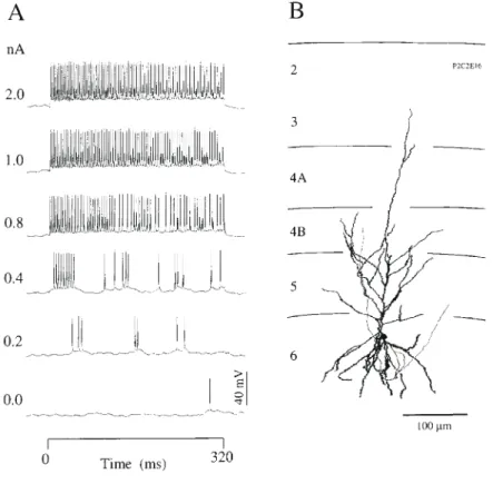
(4) Figure 1. Response of a layer 3 pyramidal neuron with a simple type (S1) receptive field (RF) to current steps. (A) Single trial responses of neuron to increasing current injections (bottom to top, amplitudes shown at left, 320 ms duration). (B) Reconstruction of the HRP-labelled neuron. Mean input impedance, 37 MΩ; ocular dominance group, 1; optimal orientation, 88° (range 31°); directionally biased.. Figure 2. Response of a layer 6 pyramidal neuron with simple type (S2) RF to 320 ms current steps. (A) Single trial responses of neuron to increasing current injections (bottom to top, amplitudes shown at left). (B) Reconstruction of the HRP-labelled neuron. Mean input impedance, 77 MΩ; ocular dominance group, 2; optimal orientation, 34° (range 68°); directionally biased.. Cerebral Cortex Jul/Aug 1998, V 8 N 5 465.
(5) Figure 3. Response of a layer 3 basket cell with simple type (S1) RF to 320 ms current steps. (A) Single trial responses of neuron to increasing current injections (bottom to top, amplitudes shown at left). (B) The morphology of the HRP-labelled neuron, dendrites shown separately on left, axon on right. Mean input impedance, 22 MΩ; ocular dominance group, 4; optimal orientation, 36° (range 33°); directionally biased.. and Martin, 1991). We thus examined the relation of the spike adaptation time constant with depth through the cortex and found a significant correlation (Fig. 6B). Neurons in the superficial layers adapted much more quickly (time constants 11.5 ± 1.3 ms, n = 20) than those in the deep layers (51.4 ± 6.4 ms, n =10). The percentage adaptation for any particular neuron was also approximately constant (Fig. 7) at all except the highest input currents, where the unadapted (maximum) discharge rate saturates and so the peak is relatively lower and the percentage adaptation is inevitably smaller. The deep layer neurons tended to have slower and weaker adaptation than the superficial layer neurons. The difference in the degree of adaptation was expressed as a percentage of (peak – adapted rate)/peak (Fig. 7). This percentage hardly changed across the range of current amplitudes for a particular neuron (Fig. 7A). On average the superficial layer neurons adapted 67%, whereas deep layer neurons adapted only 51%. Comparison of Step-current Discharge with Visually Evoked Discharge The discharge pattern of the neurons that we recorded in vivo (Figs 8A and 9A) was much more irregular than is commonly seen in vitro. These f luctuations are even more evident in the single trial responses to visual stimuli (Figs 8D and 9D), which presumably ref lect the irregularity of the synaptic drive of these neurons. Indeed, such irregularities in single trials were a major problem in the quantitative analysis of visual receptive fields and. 466 Excitatory Current Estimates of Visual Cortical Neurons • Ahmed et al.. led to the ubiquitous use of averaging techniques. It is now quite unusual to see in the literature on in vivo experiments, records like those illustrated in Figures 8 and 9. The repeatability of the in vitro responses means that single-interval current– discharge plots are conventionally used. However, because of the additional variability in the in vivo records, we averaged the firing frequency over the full period (320 ms) of the current stimulus. Data for individual superficial and deep layer neurons are illustrated in Figures 8 and 9 respectively. Our average values are slightly higher than the fully adapted discharge rate, because the early unadapted phase of the response was included. However, this difference is not very large. For a neuron with a typical time constant of adaptation of 24 ms and percentage adaptation of ∼50%, the average discharge rate is higher than the adapted discharge rate by ∼8%. The current–discharge relation of the striate neurons measured in this way for all neurons was remarkably linear (mean ± 1 SEM r2 = 0.94 ± 0.01, n = 33) over a wide range (0–3 nA) above the threshold current (Fig. 8B). The average current threshold was close to zero (mean ± 1 SEM = 0.09 ± 0.02 nA), suggesting that these neurons were poised close to their thresholds. This is unlike in vitro recordings from similar neurons, where the current threshold is usually 0.2–0.5 nA. The linear current–discharge relationship held even for neurons with the most irregular discharges, like that of the basket cell (Fig. 8). The distribution of the slopes of the current–discharge relationships is shown in Figure 10A for the population of 33 neurons. The mean of the slopes of the function was 66 spikes/s/nA (Fig. 10C, Table 1). The two neurons with the.
(6) highest slopes (Fig 10A) were outliers and were eliminated from further consideration. The laminar location of the somata of 19/31 neurons were determined histologically (Fig. 10B). The distribution of discharge rates for these identified neurons is shown in Figure 11. Superficial layer neurons were recorded in all layers except layer 1. Four neurons were located in layer 4 and all but two of the deep layer neurons were in layer 6. For these identified neurons the mean of the current–discharge slopes was 51 spikes/s/nA for superficial layer and layer 4 neurons, and 106 spikes/s/nA for the deep layer neurons (Table 1). These difference are significant (P < 0.02, Mann–Whitney U-test). If it is assumed that the average synaptic activity changes much more slowly than the time constant of adaptation, then net somatic input can be readily reckoned by using the current– discharge curve as a look-up table. In 17/31 neurons whose current–discharge relations were known, we were also able to measure the average and peak discharge rate during the optimal response to visual stimulation (e.g. Figs 8D and 9D). The average discharge rate was estimated between onset and offset of the response, and the peak rate was the maximum rate in any histogram bin within the response time. The mean peak net somatic current estimated from these values was 1.09 nA, and the mean current for the whole response was 0.64 nA (Table 1). This method gives an approximation of the net excitatory current that the spike generating mechanism is ‘seeing’. To take the temporal variation of the synaptic current into account, the method must include the kinetics of adaptation. This requires a more general, time-dependent model of the neuronal discharge, which is developed below. Transduction of Current to Spikes in Model Neurons The findings above indicate that the discharge of striate neurons scaled with their input currents, and the time constants of their transient phases were reasonably invariant with input current. These findings support the possibility that cortical neurons could be approximated as linear systems in respect of their current–discharge behaviour. However, in these experiments we measured the response of the cortical neurons to step input currents, not an impulse of input current as would be used in ideal analyses of linear systems. There are a number of practical reasons for using a step input rather than a pulse, but the most important is that the action potential output of the neuron is not a continuous variable. Instead, the action potential process effectively samples the state of excitability of the neuron. Measuring the response to a step current permits more samples to be collected and so improves the accuracy with which a single response can be assessed. Once the response to a current step has been fitted with an exponential and offset, the impulse transfer response can be obtained by differentiating the fitted function. Figure 12 outlines the procedure for obtaining the impulse transfer response, as applied to one of the model pyramidal neurons. The output of the model neuron was processed by the same methods as the biological data. The adaptation of the model neuron to the step current input was fit by the sum of an exponential and a step function (Fig. 12A) and the transfer response obtained by differentiation (Fig. 12B). As a check of the method the transfer response was convolved with the known input signal (Fig. 12C). The predicted output (Fig. 12D) was identical with the observed output of the model neuron (Fig. 12A). In this example the prediction was tested with exactly the same signal that was used to assess the transfer response and thus should provide an exact fit. If the neurons were ideal linear. systems, the predictions for arbitrary waveforms ought to be equally good. However, it is clear from the description of the experimental data that neurons, whether real or model, are only approximately linear. To test the usefulness of the approximation we have therefore examined the response of the model neuron to a number of interesting waveforms, i.e. sine waves and Hanning functions. When testing the neuron with arbitrary waveforms, we assumed that the transfer response derived from the response to a current step fully characterized the neuron’s behaviour. The response of the model neuron to a two-step input could be predicted with reasonable accuracy. Figure 13A compares the linear systems prediction for a discharge response to a two-step current input with that obtained from the model pyramidal neuron. The peak response of the neuron to the second step is less than that predicted by the transfer response. There are two reasons for such underestimates. Firstly, the transient response of the real neuron saturates at high frequencies, as seen also in Figure 13C. Secondly, reconstruction of the current input by the deconvolution method is limited by the information about the input signal that is contained in the output spike train. The prediction of the transfer response is a densely sampled (effectively continuous) function, whereas the neuronal action potential output (whether real or simulated) represents a series of discrete samples of its internal state at the points where action potentials occur and is subject to undersampling errors that depend on the frequency of discharge. When the neuronal spike rate is high relative to the frequencies of the input signal, then the input signal is densely sampled by spikes, and the reconstruction by deconvolution will be good. For a pyramidal neuron, the model indicates that the reconstruction is very good for input signal frequencies up to 10 Hz (Fig. 14A). If the input signal falls below the threshold for spike generation, or the input contains frequencies that are too high for the spike mechanism to follow, then the reconstruction deteriorates. For example, at 20 Hz (data not shown) there are only about two instantaneous frequency samples per cycle of the input signal, and so the quality of the reconstruction is poor. By 40 Hz (Fig. 14B) the output contains only one discharge frequency sample per cycle of the input (single spikes are occurring on the crests of the input signal only), and so the reconstruction recovers only an estimate of the low-frequency (DC) component of the input signal. The following examples show how the sampling problem affects the estimates of input currents in some typical experimental situations. This problem of sampling also affects the estimate of input current obtained by deconvolution. For example, the peak discharge response during fast transients underestimates the continuous response obtained from the ideal linear system (Fig. 13A,C). Consequently, the deconvolution is applied to an already degraded output signal, and so underestimates the input current in the regions of the peak response (Fig. 13B,D). An alternative way of stating this problem is that a silent neuron provides the observer with no sample of its internal state and therefore no information with which to make an estimate of the input current that it is receiving. A corollary of this point of view is that the slower the rate of action potential generation, the slower the sampling rate and so the less reliable is the estimate of the input current. The discharge of neurons cannot be negative, so the linear approximation will be violated where such behaviour is predicted. The absence of negative discharge is only a minor limitation when it relates to the prediction of an output response. Cerebral Cortex Jul/Aug 1998, V 8 N 5 467.
(7) Figure 4. Spike frequency responses of superficial and deep layer cortical neurons to current steps (amplitudes in nA shown at right). Measured instantaneous frequencies are indicated by open circles. The continuous curve through the data points is the best-fit single exponential decay to a constant. The data illustrate the fast adaptation characteristics of superficial layer neurons (A: layer 3 pyramid, simple type S1 RF, mean time constant of adaptation = 12.1 ms, mean r2 = 0.81; C: layer 2 neuron, standard complex type CST RF, mean time constant of adaptation = 9.4, mean r2 = 0.81) compared with the deep layer pyramidal neuron (B: layer 6, simple type S2 RF, mean time constant of adaptation = 35.9 ms, mean r2 = 0.71).. of the neuron — in practice a zero discharge is a good enough prediction. However, the inability to represent negative output rates has much deeper consequences when the output of the neuron must be deconvolved with the transfer response to estimate the input current. Obviously, if the output is required to go negative but cannot, then the estimation of input will be inaccurate in those regions. An example of the kind of problem that can arise is seen in Figure 13B. The output response (Fig. 13A, thin line) goes to zero rather than negative. But the deconvolution makes a distinction between these two cases. If the discharge signal is zero rather than negative, the deconvolution reports that the input signal is relaxing back to zero more slowly than it in fact does (Fig. 13B, thick line). Various strategies could be used to minimize these inaccuracies. For example, estimates of input current could be. 468 Excitatory Current Estimates of Visual Cortical Neurons • Ahmed et al.. ignored where the discharge rate is either very low or zero. Assumptions about the behaviour of the negative-going output could be made if some properties of the input signal were known a priori. For example, if the input signal is known to be rectangular, then the trailing artefact can be neglected. Another strategy would be to apply negative-going input signals in the presence of a positive background current that would offset the output discharge and prevent it falling to zero. An example of this strategy is shown in Figure 14A. The input signal is a 0.3 nA 10 Hz sine wave, and would normally lead to periodic phases of zero discharge during which the estimated input current would be uncertain. However, when the sine wave is applied in the presence of a 1.0 nA offset current, the discharge is always greater than zero and the output of the neuron agrees well with the ideal linear prediction (thick line, Fig 14A, middle). But more.
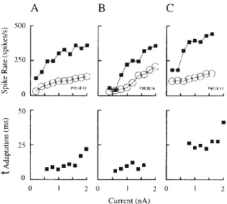
(8) Figure 5. Current–discharge relations and adaptation time constants for three neurons (A: layer 3 pyramid, S1 RF; B: layer 6 pyramid, S2 RF; C: layer 2 neuron, CST RF) recorded in vivo in cat striate cortex. The instantaneous spike frequency for the first spike interval and the adapted discharge frequency are denoted by the filled squares and open circles respectively. The fitted time constants of adaptation (τadaptation) over a range of current steps are shown below. Figure 6. The time constants of adaptation for the 40/45 neurons for which single exponential decays could be fitted. (A) Population distribution of time constants (class interval 5 ms). The time constant for an individual neuron was taken as the average value of the exponential functions obtained at different test currents. (B) Relationship between the adaptation time constant (τadaptation) of a neuron and its laminar location. Filled squares, neurons whose location was inferred from electrode depth measurement alone (morphology unknown); filled circles, morphologically identified pyramidal neurons; open circle, morphologically identified basket cell. The mean (± 1 SEM) time constants of adaptation for superficial and deep layer neurons were, respectively, 11.5 ± 1.3 ms and 51.4 ± 6.4 ms. P < 0.001, t-test.. importantly, the output of the neuron can be deconvolved to provide a good estimate of the input sine wave current (Fig. 14A, lower trace, thin line, input; thick line, estimate). However, even in the presence of an offset, the frequency of firing of the neuron limits the fidelity of the reconstruction. A 40 Hz input signal is not recovered (Fig. 14C).. Figure 7. Percentage adaptation of discharge rate observed in cortical neurons in vivo. Adaptation expressed as a percentage of (peak – adapted)/peak ). (A) Examples for superficial (circles) and deep (filled squares) layer neurons. All deep layer neurons showed a systematic decrease in percentage adaptation with increasing current. (B) Data for all 40 neurons (class interval of 0.4 nA, bars are ± 1 SEM). Statistically significant differences (P < 0.05) are indicated by asterisks. (C) Distribution of mean values of percentage adaptation for all 40 neurons (mean = 63.1, ± 1 SEM = 2.5), and according to their superficial (mean = 67.1, ± 1 SEM= 3.0, n = 20) and deep (mean = 51.2, ± 1 SEM= 4.9, n = 10) layer locations (P = 0.01, t-test).. Figure 15 shows the estimates obtained by the transfer response method for input currents of the form expected during visual input, i.e. smoothly increasing and decreasing currents (Douglas et al., 1991). The input currents were modelled as Hanning functions of various amplitudes (Fig. 15, thin lines). These signals were injected in the model neuron. The action potential discharges were recovered, and deconvolved with the neuron’s transfer response to yield estimates of the input current (Fig. 15, thick lines). The responses scale well with the magnitude of the input current, confirming the suitability of the linear systems approximation. In all three cases the input currents are slightly underestimated as the discharge rate of the neuron decreases. The underestimate is worst for the smallest amplitude Hanning input. The underestimate is due to the dependence of the adaptation time constant on discharge rate. For the smallest Hanning input the neuron is always discharging at a much lower rate than elicited during the evaluation of its transfer response by a 1 nA step function. Consequently, the neuron’s effective adaptation time constant will be less than the value used in the transfer response. Because the neuron adapts more quickly, its actual discharge sags below the predicted value. Conversely, because the transfer response assumes a longer time constant of adaptation, the deconvolution underestimates (Fig. 15A, thick line) the current required to achieve the ideal discharge (Fig. 15A, thin line). Nevertheless, the simulations show that given a reasonably linear neuron, the response of the neuron to input currents of arbitrary waveforms can be predicted with good accuracy. Net Somatic Current During Visual Stimulation The simulations with model neurons show that the transfer response method provides a close approximation to the ideal responses predicted by linear systems theory. In this final section we apply the technique to real cortical neurons in order to estimate the net current that produces the discharge during visual stimulation. In eight neurons for which we were able to. Cerebral Cortex Jul/Aug 1998, V 8 N 5 469.
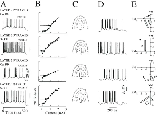
(9) Figure 8. Current–discharge characteristics and visual responses of neurons in the superficial layers of cat striate cortex (three pyramidal neurons and one basket cell). (A) Single traces recorded during intracellular current injection of 1.0 nA. Simple type receptive field (RF) denoted by S; subscripts denote the number of discharge centres; standard complex type denoted by CST. Latency of response of cells to electric stimulation at site OR1 were 3.3 ms (P5C1E13), 0.9 ms (P7C1E13), 3 ms (P3C2E16) and 1.9 ms (P9C1E14) (B). Current–discharge relationships for each of the neurons at left. Each point (filled square) represents the spike rate averaged over the duration of intracellular current step. Solid line, best fit linear regression. Horizontal arrow, the mean spike rate during visual drive. (C) Anatomical diagram showing the location in the cortex of the somata of the recorded neurons. (D) Single traces of the response to an optimally oriented bar stimulus. (E) The receptive field and preferred stimulus for the neuron. VM, vertical meridian (degrees); HM, horizontal meridian; arrow, preferred direction of bar movement eliciting the optimal response.. Figure 9. Current–discharge characteristics and visual responses for deep layer pyramidal neurons. Details as for Figure 8. Latency of response of cells to electric stimulation at site OR1 were 2 ms (P4C3E12), 5 ms (P6C4E15), 2.7 ms (P1C1E16) and 2.2 ms (P2C2E16).. 470 Excitatory Current Estimates of Visual Cortical Neurons • Ahmed et al..
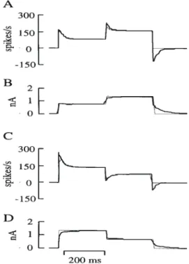
(10) Figure 10. Current–discharge relation in neurons. (A) Distribution of slopes in a sample of 31 neurons. (B) Relationship between location of the soma and the slopes of the current–discharge responses in 19 neurons labelled intracellularly with horseradish peroxidase (see Fig. 4). (C). Linear regression onto the current–discharge data (solid line, slope = 65.9 ± 6.7 SEM spikes/s/nA, n = 31). Dashed lines, 95% confidence limits. Open and filled diamonds, mean and peak responses of neurons to visual stimulation respectively. The somatic currents that evoke these levels of spike activity are indicated by the vertical dashed lines. Mean and peak response currents were 0.64 and 1.1 nA.. Table 1 Characteristics of striate neurons Parameter. Units. Current–frequency (f–I) slope spikes/s/nA. peak Isyn. average Isyn. peak Isyn (deconvolution). nA. Population. Mean. SEM. n. all superficial deep all superficial deep all superficial deep all. 65.9 50.7 105.7 1.1 1.1 0.80 0.64 0.62 0.54 0.62. 6.7 5.9 19.9 0.14 0.18 0.33 0.08 0.10 0.15 0.15. 31 13 6* 17 10 4a 17 10 4a 8. Figure 12. Transfer response of a model layer 2/3 pyramidal neuron. (A) Exponential adaptation function fitted to instantaneous discharge frequency of the neuron in response to the intrasomatic current step shown in (C). (B) Transfer response obtained by differentiating the fitted function of (A). (C) A 1 nA intrasomatic current step. (D) Predicted output obtained by convolution of (B) with (C). The predicted response agrees exactly with the observed response (A).. *P = 0.05; anon-significant (P values were calculated with respect to superficial neurons in each parameter category).. Figure 11. The current–discharge data separately plotted for superficial (A) and deep (B) layer neurons. The mean (± 1 SEM) slopes for superficial and deep layer neurons were 51 ± 6 (n = 13) and 106 ± 20 (n = 6) spikes/s/nA respectively (P < 0.02, Mann–Whitney U-test). The mean and peak discharge responses to the optimal visual stimulus are indicated by the open and filled diamonds. These responses correspond respectively to net somatic currents of 0.62 and 1.13 nA for superficial neurons (n = 10), and 0.54 and 0.80 nA for deep layer neurons (n = 4).. Figure 13. Simulation of responses to staircase input to a layer 2/3 pyramidal neuron. (A) Instantaneous discharge frequency (thin line) in response to the intrasomatic current signal shown in (B). Ideal output response (thick line), predicted by convolution of the neuron’s transfer response with the same intrasomatic current signal applied to the neuron. (B) Estimate of the somatic input current (thick line), obtained by deconvolution of the neuron’s output discharge with its transfer response. The input current is overestimated in the period following the offset of the test signal, because the negative discharge predicted by the transfer response (thick line in A) is not measurable in a real neuron. Thin line, ideal input current: 0.8 nA stepped to 1.5 nA. (C) As for (A), but for reversed order of staircase current input. (D) As for (B), but for reversed order of staircase current input. Here the model (thick line in D) correctly predicts the input current for the step from 1.5 to 0.8 nA, because the discharge remains positive, but overestimates the current when the current steps from 0.8 nA to zero.. Cerebral Cortex Jul/Aug 1998, V 8 N 5 471.
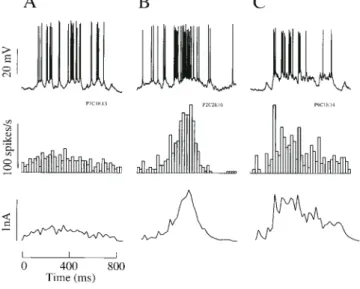
(11) Figure 14. Simulation of responses of a pyramidal neuron to intrasomatic current injection of 10 Hz (A) and 40 Hz (B) sinusoids superimposed on a step. The input signal of a 1 nA step, 0.3 nA amplitude sine wave of (A) 10 Hz and (B) 40 Hz, is indicated as the thin line in lower panel. The somatic membrane potential of the model layer 5 pyramidal cell is shown in the top panel. Measured instantaneous discharge frequencies (asterisks joined by thin lines) are plotted in the center panel. The instantaneous frequencies are interpolated by a cubic spline (thick line, middle panel). The interpolated signal was deconvolved with the neurons’ transfer response to obtain the estimated input current (thick trace, lower panel). The deconvolution method provides a good estimate (thick line) of the 10 Hz input (thin line, lower panel in A), but recovers only the low-frequency features (thick line) of the 40 Hz input signal (thin line, lower panel in B).. Figure 16. Visual evoked responses and input currents for superficial (A) and deep layer pyramidal (B) neurons and the layer 3 basket cell (C). Top row are single traces of the neuronal discharge during the passage of an optimal stimulus across the receptive field. Middle row are the peristimulus time histograms of the spike discharge (10 trials, bin width 20 ms). The lower traces are the estimates of the somal currents derived from the transfer response. Time scale applies to all rows.. derive an impulse response, we also recorded their responses to visual stimulation. These data were used to obtain estimates of the net input currents by deconvolution. The visual response was usually to a bar passing across the receptive field of the neuron with preferred orientation and velocity and direction. Three examples are shown in Figure 16. The upper traces show individual trials during which the neurons responded to visual stimulation. The discharge of the neurons recorded in vivo under these conditions is characteristically variable from trial to trial, and so we averaged the response over a number of trials to obtain the best estimate of the discharge rate in response to visual stimulation (rate histograms, Fig. 16). Averaging necessarily smooths the form of the output signal, and so high-frequency f luctuations are filtered out. The lower traces of Figure 16 show the estimates of the net somatic current obtained by the deconvolution technique that evoked the response of the neurons to optimal visual stimulation. The three highest peak currents were in excess of 1 nA. The three smallest currents were ∼0.3 nA and all were recorded from layer 6 pyramidal cells. The average (± SEM) estimated peak somatic current of the eight neurons was 0.62 ± 0.15 nA and the average net charge delivery to the soma was 0.23 ± 0.05 nC.. Discussion. Figure 15. Simulation of responses of layer 2/3 pyramidal neuron to 0.6, 1.0 and 1.5 nA amplitude Hanning input currents. (A) Instantaneous discharge frequencies (thick line) in response to the three intrasomatic current signals. Ideal output responses (thin lines) predicted by convolving the neuron’s transfer response with the same intrasomatic current signals applied to the neuron. (B) Estimate of the somatic input currents (thick lines), obtained by deconvolving the neuron’s output discharges with its transfer response. Thin lines, ideal input currents.. 472 Excitatory Current Estimates of Visual Cortical Neurons • Ahmed et al.. Our results show that pyramidal neurons observed in cat visual cortex in vivo exhibit the same basic relationship between excitatory current and firing frequency and the same process of adaptation that have been observed in neurons in vitro. In this respect the membrane properties appear to be preserved in vivo. Qualitatively similar findings have been reported in the cat for neurons in motor cortex (Calvin and Sypert, 1976; Baranyi et al., 1993) and association cortical areas 5 and 7 (Nunez et al., 1993). Clearly, the firing patterns seen in vitro are more reproducible trial to trial (e.g. Mainen and Sejnowski, 1995; Nowak et al., 1997) than in vivo, and this difference may be attributed in part at least to synaptic activity. A similar observation has been reported for cat visual cortex in vivo (Gray.
(12) and McCormick, 1996; Bringuier et al., 1997). We did not use the lengthy test periods that were required to see the slow changes that Schwindt et al. (1988a,b) report in vitro. Our obser vations were made over the first 300 ms of adaptation, during which the major changes in firing frequency occur. During this period, adaptation in both hippocampal and neocortical neurons is dominated by just one or perhaps two calcium-dependent potassium currents (Connors et al., 1982; Schwindt et al., 1988a,b; Berman et al., 1989; Aicardi and Schwartzkroin, 1990; Segal, 1990; Staley et al., 1992). Studies of cortical slices in vitro indicate that the potassium currents are sensitive to various putative neurotransmitters, including norepinephrine, acetylcholine and serotonin (see reviews by Nicoll et al., 1990; McCormick, 1992). We found that the basket cell produced fast spikes and had high frequencies of firing and showed some spike rate adaptation at high currents. None of the three identified basket cells recorded by Azouz et al. (1997), however, had the bursty discharge patterns seen in this basket cell. Steriade et al. (1998) have reported similar patterns in corticothalamic and ‘local cortical interneurons’ of motor and association cortex. However, their morphological data indicated that all of their neurons were spiny or sparsely spiny, not smooth neurons like basket cells. In our sample of superficial and deep layer pyramidal cells we did not observe burst discharges of spikes at frequencies of 20–70 Hz in response to visual stimulation (Hubel and Wiesel, 1965; Gray and McCormick, 1996). Low-frequency (7–20 Hz) oscillations have been reported by Bringuier et al. (1997) in response to visual stimulation. We have reported that low-frequency oscillations (mean = 9.5 Hz, n = 31) can be evoked by electrical pulse stimulation of the optic radiations combined with visual stimulation (A hmed et al., 1994), suggesting that this may be one natural resonance frequency of the circuit. We found that the adaptation of the spike discharge over time can be well-fitted by the sum of a single exponential and a constant. This is surprising in view of the number of different conductances that contribute to the dynamics of action potential generation in cortical neurons (Crill et al., 1986; Flatman et al., 1986; Franz et al., 1986; Sutor and Zieglgansberger, 1987; Spain et al., 1991; Traub et al., 1991). Lorenzon and Foehring (1992) recorded from human neocortical tissue and reported that the discharge in response to currents of 1–2 nA could be fitted by the sum of two exponentials. Although we found that the fits with two exponentials made little improvement on fits with one exponential, the time constants Lorenzon and Foehring (1992) extracted (range 10–21 ms for the first time constant, 70–159 ms for the second) are broadly consistent with our findings. In vitro studies have not reported a relationship between laminar location and the time constant and magnitude of adaptation. We found in vivo that superficial layer pyramidal neurons have short adaptation time constants (3–24 ms), whereas the deep layer neurons have longer ones (24–75 ms). Moreover, the deep layer neurons adapt less completely than superficial layer neurons. We do not know why these differences exist in the cat visual cortex. They cannot be due to systematic variations in the input impedance between deep and superficial layer neurons, because the input conductance of the neuron during discharge is dominated by the average spike conductance. It is possible that these correlations could be due to surface/volume ratio differences between the superficial and deep layer neurons. The calcium compartment that affects adaptation is thought to be only a thin shell beneath the membrane (Yamada et al., 1989), and the size of this shell would. tend to scale with surface area of the soma rather than its volume. This would make the calcium dynamics (and adaptation) relatively insensitive to somatic diameter. It seems, then, that the calcium dynamics must be fundamentally different in deep layer neurons than in superficial layer neurons. There is some evidence for such a difference within the population of layer 5 pyramidal neurons. Some of these neurons exhibit bursting discharges that depend on the expression of calcium conductances (Silva et al., 1991), potassium conductances (Schwindt et al., 1988a,b) or calcium- dependent potassium conductances (Berman et al., 1989; Friedman and Gutnick, 1989; Silva et al., 1991). However, most of the deep layer neurons recovered were in layer 6, where bursting neurons have not been reported in vitro. The current–discharge relation of striate neurons is remarkably linear over a 0–2 nA range of somatic input current, with an average slope of 66 spikes/s/nA. The large Betz cells of the cat motor cortex in vitro have a f latter slope in their current discharge (∼20 spikes/s/nA), but as Schwindt (1992) has noted, also have remarkably linear input–output relationships given the number of non-linear conductances underlying the discharge pattern. Unlike neurons recorded in vitro, which have threshold currents of ∼0.4 nA (Connors et al., 1982; Mason and Larkman, 1990), the striate neurons in vivo are poised close to their threshold (Berman et al., 1991; Douglas et al., 1991). This finding is consistent with the observation that many cortical neurons are spontaneously active (Gilbert, 1977; Leventhal and Hirsch, 1978), and with the membrane potentials observed in our intracellular studies (Berman et al., 1991; Douglas et al., 1991). The simple linear behaviour of the neurons suggested that the current–discharge curve could be used to estimate directly the net somatic current resulting from synaptic activity on the dendrites. We have assumed that the action potentials are generated close to the soma where the recording pipette is located. Delivering current into the soma from a recording pipette may not be identical to the case where the current is delivered to the soma from synapses. The dendrites with active synapses will be more depolarized than the soma and the dendritic voltagesensitive conductances are likely to be active. This means that the soma may experience a larger dendritic conductance load in the synaptically driven case than the pipette-driven case. These differences are only relevant below threshold. In motoneurons these differences were found to be so small that synaptic and injected current have an equivalent effect in driving discharge (Schwindt and Calvin, 1973). More recently Powers et al. (1992) and Schwindt and Crill (1996) have used a modified voltageclamp technique to measure the synaptic current delivered to the somata of neurons held at resting potential. They found that the synaptically evoked steady-state discharge of motoneurons is fully explained by the measured synaptic current, corrected for the change in driving potential that occurs during sustained discharge. The spike itself did not disrupt the transfer of current from dendrites to soma. Indeed, the spike mechanism acts as an imperfect voltage-clamp that restricts the somatic potential to a range of ∼10mV above the voltage threshold for discharge (Bernander et al., 1991; Holt and Koch, 1997) and so sinks as much current as the dendrites (or an intrasomatic electrode) will deliver. Thus, once the action potential discharge begins, the average spike conductances will contribute to the conductance load. In this respect, a space-clamp of the entire neuron would produce misleading results in the present context, because the. Cerebral Cortex Jul/Aug 1998, V 8 N 5 473.
(13) measurements of the net current would be made with an inappropriate dendritic conductance load. Using the simple current–discharge relation as a means of calibrating the current delivery to the cortical neurons, we estimated the average and peak net current delivered to these neurons during the passage of a bar stimulus across their receptive field was 0.64 and 1.1nA respectively. It should be emphasized that this method estimates only the net current delivered to the soma through the action of the active synapses. It is insensitive to changes in the contributions of individual synapses, or groups of synapses, that may occur due to nonlinear interactions between synapses (e.g. Shepherd et al., 1985) or changes in the electromorphology of the neuron (Rall 1964; Jack et al., 1975; Bernander et al., 1991). It also does not discriminate between excitatory and inhibitory currents; it only estimates the net current arriving at the soma. This net somatic current is the current delivered to the soma from the dendrites (or an intra-somatic pipette). It will be dissipated through the spike conductances, the adaptation conductances and the passive input conductance at the soma. Powers et al. (1992) used a similar approach to our first approximation to estimate the effective synaptic current from the discharge of motoneurons. In their method the input current is computed from the steady-state discharge only, and adaptation transients are ignored. This method provides suitable estimates when the input to the neuron changes much more slowly than the time constants of adaptation. However, the dynamic component cannot be entirely neglected in the neurons of striate cortex, because the discharge of simple cells is modulated by moving sinusoidal contrast gratings up to temporal frequencies of 8 Hz (Maffei and Fiorentini, 1973; Ikeda and Wright, 1975; Tolhurst and Movshon, 1975; Movshon et al., 1978). At these high frequencies, adaptation mechanisms will affect the discharge of the neurons. Another approach to this problem was taken by Awiszus (1989, 1990, 1992), who described various methods for inferring the strength of synaptic input from action potential output, and so would be sensitive to the temporal form of the input. His first method makes use of a full Hodgkin–Huxley type simulation of action potential generation, and estimates the input current by successive approximation. At the end of each trial, the output of the model is compared to the experimentally observed discharge and the profile of the estimated current is corrected. Typically, 100 such iterations must be performed to achieve convergence. Moreover, successful convergence depends on there being a good match between the parameters of the Hodgkin–Huxley model and the particular real neuron being examined. This match must be determined by experiment. Clearly, this method of inferring input current does not lend itself to real-time investigations. Awiszus’ second method was based on the leaky integrator model of action potential discharge. An analytical reconstruction operator was used to recover the input current. The second method was simpler than the first, but its application is limited to the rare case of neurons that can be well modelled by a leaky integrator. Our second method improves on the steady-state estimate by using the time-course of adaptation to obtain the transfer response of the neuron. It takes account of the adaptive behaviour of the neuron when estimating the somatic current so that transient somatic currents can also be recovered. Unlike Awiszus’ approach, our method makes no assumptions about the biophysics that underlie the neuronal response and our estimates can be made very rapidly. It could be calculated and used during. 474 Excitatory Current Estimates of Visual Cortical Neurons • Ahmed et al.. an impalement, for example. It is important to emphasize that the transfer response method is only valid if the behaviour of the neuron is approximately linear. This linearity has to be established for each class of neuron. As we have shown, many striate cortical neurons do behave approximately linearly with respect to their current–discharge behaviour. We have also shown that the form of neuronal adaptation is a simple exponential plus a constant, and that although the time constant of decay is not identical for all input currents, the change is sufficiently small for the linear approximation to remain useful, as we have demonstrated by simulation. The most significant error in the estimation of input current by the deconvolution technique occurs because the discharge rate of the neuron cannot go negative. This leads to an overestimation of the input current when the discharge of the neuron is low or zero. The problem can be overcome by applying a depolarizing offset current to the neuron so that its change in discharge is biased around the offset (Fig. 14). In those cells for which we were able to estimate the net peak current by both the current–discharge method and the deconvolution method, we found that the former method overestimated the peak current by ∼40% with respect to values calculated by deconvolution. This difference is explained by the differentiating response of the neuron to transients: methods that depend on steady-state behaviour will overestimate the net input currents during transients. This is evident from the current–discharge curves generated by a step input of current. The transfer response method yields an average estimate of ∼0.6 nA for the net peak current delivered to the soma during preferred motion of a bar stimulus. Three of the eight cells examined had peak currents of 1 nA or more. This indicates a substantial excitatory input to the neurons. We estimate that the average charge delivered to the soma during the visual response was in the region of 0.23 nC. From hippocampal neuron cultures the estimated charge provided by a single excitatory synapse is ∼0.2 pC (Bekkers and Stevens, 1989). If this is an appropriate number for cortical neurons, and if the total charge is contributed by purely synaptic events, then at least 1000 excitatory synaptic events must contribute to the observed visual response. Since each presynaptic neuron may fire at frequencies of between 10 and 50 Hz during visual stimulation, the number of active excitatory synapses may only be 100 or less. However, if inhibitory synapses are simultaneously active during visual stimulation, because of the recurrent circuitry (Douglas et al., 1989, 1991), more excitatory synapses would be required. Nevertheless, even were the actual number of active excitatory synapses larger by a factor of 5–10, this would still be a fraction of the total excitatory synapses (>5000) formed with the neuron. These estimates also raise the question as to what degree the net current arriving at the soma is also conditioned by mechanisms that limit the total current transmitted from the dendrites to the soma. There is recent evidence from hippocampal slice preparations (Hoffman et al., 1997) for such a gain control that is mediated through the A-type potassium channels in the dendrites, which act to reduce the amplitude of the excitatory synaptic currents. It now needs to be established what are the contribution of the total synaptic current that arises from the different sources of synapses converging on single neurons and how the active conductances in the dendrites of neocortical neurons might shape the synaptic current delivered to the soma from the dendrites during natural stimulation..
(14) Notes Supported by the Swiss National Science Foundation (SPP), EU, Human Frontiers Science Program, and MRC (UK). Address correspondence to Kevan A.C. Martin, Institute of Neuroinformatics, ETH/University of Zurich, Gloriastrasse 32, CH-8006, Zurich, Switzerland. Email: [email protected].. References A hmed B, Anderson, JC, Douglas RJ, Martin K AC, Whitteridge D (1993) A method of estimating net somatic input current from the action potential discharge of neurones in the visual cortex of the anaesthetized cat. J Physiol 459:134P. Ahmed B, Anderson JC, Douglas RJ, Martin K AC, Whitteridge D (1994) Evidence for synchronization in active populations of visual cortical cells of the anesthetized cat due to pulse activation of thalamic afferents. J Physiol 480:106P. Aicardi G, Schwartzkroin PA (1990) Suppression of epileptiform burst discharges in CA3 neurons of rat hippocampal slices by the organic calcium channel blocker, verapamil. Exp Brain Res 81:288–296. Awiszus F (1989) On the description of neuronal output properties using spike train data. Biol Cybern 60:323–333. Awiszus F (1990) On a method to infer quantitative information about the current driving action potential generation from neuronal spike train data. Biol Cybern 62:249–257. Awiszus F (1992) Analytical reconstruction of the neuronal input current from spike train data. Biol Cybern 66:537–542. Azouz R, Gray CM, Nowak LG, McCormick DA (1997) Physiological properties of inhibitory interneurons in cat striate cortex. Cereb Cortex 7:534–545. Baranyi A, Szente MB, Woody CD (1993) Electrophysiological characterization of different types of neurons recorded in vivo in the motor cortex of the cat. II. Membrane parameters, action potential, current-induced voltage responses and electrotonic structures. J Neurophysiol 69: 1865–1879. Bekkers JM, Stevens CF (1989) NMDA and non-NMDA receptors are co-localized at individual excitatory synapses in cultured rat hippocampus. Nature 341:230–233. Berman NJ, Bush PC, Douglas RJ (1989) Adaptation and bursting in neocortical neurones may be controlled by a single fast potassium conductance. Quart J Exp Physiol 74:223–226. Berman NJ, Douglas RJ, Martin KAC, Whitteridge D (1991) Mechanisms of inhibition in cat visual cortex. J Physiol 440:697–722. Bernander O, Douglas RJ, Martin K AC, Koch C (1991) Synaptic background activity inf luences spatiotemporal integration in single pyramidal cells. Proc Natl Acad Sci USA 88:11569–11573. Bringuier V, Fregnac Y, Baranyi A, Debanne D, Shulz D (1997) Synaptic origin and stimulus dependency of neuronal oscillatory activity in the primary visual cortex of the cat. J Physiol 500:751–774. Bush PC, Douglas RJ (1991) Synchronization of bursting action potential discharge in a model network of neocortical neurons. Neural Comp 3:19–30. Calvin WH, Sypert G (1976) Fast and slow pyramidal tract neurons: an intracellular analysis of their contrasting repetitive firing properties in the cat. J Neurophysiol 39:420–434. Carandini M, Mechler F, Leonard CS Movshon JA (1996) Spike train encoding by regular-spiking cells of the visual cortex. J Neurophysiol 76:3425-3441. Connors BW, Gutnick MJ, Prince DA (1982) Electrophysiological properties of neocortical neurons in vitro. J Neurophysiol 48: 1302–1320. Crill WE, Schwindt PC, Flatman JA, Stafstrom CE, Spain W (1986) Inward currents in cat neocortical neurons studied in vitro. Adv Exp Med Biol 203:401–411. Douglas RJ, Martin K AC (1991) A functional microcircuit for cat visual cortex. J Physiol 440:735–769. Douglas RJ, Martin K AC (1992) Exploring cortical microcircuits: a combined anatomical, physiological, and computational approach. In: Single neuron computation (Zornetzer S, Davis J, McKenna T, eds), pp. 381–412. Boston, MA: Academic Press. Douglas RJ, Martin K AC, Whitteridge D (1989) A canonical microcircuit for neocortex. Neural Comput 1:480–488. Douglas RJ, Martin KAC, Whitteridge D (1991) An intracellular analysis of the visual responses of neurones in cat visual cortex. J Physiol 440:659–696.. Douglas RJ, Koch C, Mahowald M, Martin K AC, Suarez H (1995) Recurrent excitation in neocortical circuits. Science 269:981–985. Flatman JA, Schwindt PC, Crill WE (1986) The induction and modification of voltage-sensitive responses in cat neocortical neurons by N-methyl-D-aspartate. Brain Res 363:62–77. Franz P, Galvan M, Constanti A (1986) Calcium-dependent action potentials and associated inward currents in guinea-pig neocortical neurons in vitro. Brain Res 366:262–271. Friedman A, Gutnick MJ (1989) Intracellular calcium and control of burst generation in neurons of guinea-pig neocortex in vitro. Eur J Neurosci 1:374–381. Gilbert CD (1977) Laminar differences in receptive field properties of cells in cat primary visual cortex. J Physiol 268:391–421. Granit R, Kernell D, Shortess GK (1963) Quantitative aspects of repetitive firing of mammalian motoneurones, caused by injected currents. J Physiol 168:911–931. Granit R, Kernell D, Lamarre Y (1966a) Algebraical summation in synaptic activation of motoneurones firing within the ‘primary range’ to injected currents. J Physiol 187:379–399. Granit R, Kernell D, Lamarre Y (1966b) Synaptic stimulation superimposed on motoneurones firing in the ‘secondary range’ to injected current. J Physiol 187:401–415. Gray CM, McCormick DA (1996) Chattering cells: superficial pyramidal neurons contributing to the generation of synchronous oscillation in the visual cortex. Science 274:109–113. Hamill OP, Huguenard JR, Prince DA (1991) Patch-clamp studies of voltage-gated currents in identified neurons of the rat cerebral cortex. Cereb Cortex 1:48–61. Hines M (1989) A program for simulation of ner ve equations with branching geometries. Int J Biomed Comput 24:55–68. Hines M (1993) NEURON — a program for simulation of nerve equations. In: Neural systems: analysis and modeling (Eeckman F, ed.), pp. 127–136. Dordrecht: Kluwer. Hoffman DA, Magee JC, Colbert CM, Johnston D (1997) K+ channel regulation of signal propogation in dendrites of hippocampal pyramidal neurons. Nature 387:869–875. Holt GR, Koch C (1997) Shunting inhibition does not have a divisive effect on firing rates. Neural Comput 9:1001–1013. Holt GR, Softky WR, Koch C, Douglas, RJ (1996) Comparison of discharge variability in vitro and in vivo in cat visual cortical neurons. J Neurophysiol 75:1806–1814. Hubel DH, Wiesel TN (1965) Receptive fields and functional architecture in two nonstriate visual areas (18 and 19) of the cat. J Neurophysiol 28:229–289. Ikeda H, Wright MJ (1975) Spatial and temporal properties of ‘sustained’ and ‘transient’ neurones in area 17 of the cat’s visual cortex. Exp Brain Res 22:363–383. Jack JJB, Noble D, Tsien, RW (1975) Electric current f low in excitable cells. Oxford: Oxford University Press. Komatsu Y, Nakajima S, Toyama K, Fetz EE (1988) Intracortical connectivity revealed by spike-triggered averaging in slice preparations of cat visual cortex. Brain Res 442:359–362. Leventhal AG, Hirsch HVB (1978) Receptive-field properties of neurons in different laminae of visual cortex of the cat. J Neurophysiol 41:948–962. Lorenzon NM, Foehring RC (1992) Relationship between repetitive firing and afterhyperpolarizations in human neocortical neurons. J Neurophysiol 67:350–363. Maffei L, Fiorentini A (1973) The visual cortex as a spatial frequency analyzer. Vis Res 13:1255–1267. Mainen ZF, Sejnowski TJ (1995) Reliability of spike timing in neocortical neurons. Science 268:1503–1506. Martin K AC (1984) Neuronal circuits in cat striate cortex. In: Cerebral vortex, Vol. 2: Functional properties of cortical cells (Jones EG, Peters A, eds), pp. 241–284. New York: Plenum Press. Martin K AC, Whitteridge D (1984) Form, function and intracortical projections of spiny neurones in the striate visual cortex of the cat. J Physiol 353:463–504. Mason A, Larkman A (1990) Correlations between morphology and electrophysiology of pyramidal neurons in slices of rat visual cortex. II. Electrophysiology. J Neurosci 10:1415–1428. Mason A, Nicoll A, Stratford K (1991) Synaptic transmission between individual pyramidal neurons of the rat visual cortex in vitro. J Neurosci 11:72–84. McCormick DA (1992) Neurotransmitter actions in the thalamus and. Cerebral Cortex Jul/Aug 1998, V 8 N 5 475.
Figure
+2
Documents relatifs