Bayesian Inference on Major Loci in Related Multigeneration
Selection Lines of Laying Hens
C. Hagger,*
,1L. L. G. Janss,‡ H. N. Kadarmideen,† and G. Stranzinger*
*Breeding Biology Group and †Statistical Animal Genetics Group, Institute of Animal Science, Swiss Federal Institute of Technology, ETH-Zentrum, CH-8092 Zu¨rich, Switzerland; and ‡Division of Animal Sciences, Institute
for Animals Science and Health, ID-Lelystad, PO Box 65, 8200 AB Lelystad, The Netherlands
ABSTRACT A mixed inheritance model, postulating a polygenic effect and differences between the 3 genotypes of a biallelic locus, was fitted separately to the data of 2 multigeneration selection lines and a control evolving from a common base population. Inferences about the model were drawn from the application of the Gibbs sampler. Body weight at 20 and 40 wk (BW20, BW40) and average egg weight to 40 wk (EW40) were included in the analyses. Significance of differences between posterior means of parameters was established by comparing their 95% highest probability density regions. Significant (P< 0.05) additive and dominance effects due to the genotypes at the major locus were found for all traits. The allele causing a lower trait value was the (partial) dominant one in all traits, leading to a negative dominance effect. The additive variance due to the major locus was also
(Key words: mixed inheritance, additive dominance effect, biallelic major locus, body weight, egg weight) 2004 Poultry Science 83:1932–1939
INTRODUCTION
The mixed inheritance model assumes that the genetic influence on a trait is of 2 distinct parts, a polygenic one (infinitesimal model) and, in the simplest case, one from a locus with a large effect (major locus) bearing 2 segregat-ing alleles. This assumption has the consequence that the distributions of phenotypes and genotypes in a popula-tion are mixtures of several distribupopula-tions. The shape of the combined distributions is dependent upon the inheri-tance mode at the major locus, the associated allele fre-quency, and the size of the effect of the major locus on the phenotype of the trait. The shape of the within-family distribution will vary depending on the genotypes of the parents. In the absence of genetic markers, the phenotypic distributions of traits thus contain the necessary informa-tion to verify the mixed inheritance model for a particular
2004 Poultry Science Association, Inc. Received for publication March 31, 2004. Accepted for publication August 3, 2004.
1To whom correspondence should be addressed: hagger@inw.
agrl.ethz.ch.
1932
significant, i.e., greater than zero (P< 0.05) in all traits, whereas the dominance variance was only important for EW40. With the exception of the residual variances of one selection and the control line, no (P> 0.05) differences of posterior means of any parameter could be observed between lines. No significant genotypic or polygenic se-lection response was found for BW40. On the contrary, both genetic responses were found significant for EW40 in the selected lines, but not in the control. No differences (P> 0.05) between lines could be observed for the derived frequencies of the allele causing the higher trait value and the frequencies of one homozygote and the heterozygote genotypes at the major locus. The detection of a major locus with relatively modest effect confirmed that this type of analysis with data from selected lines was in-deed powerful.
trait in a particular population. Segregation analysis (Els-ton and Stewart, 1971), a likelihood based method, is a powerful tool for the detection of major loci in certain, mostly human, data sets. It is, however, not applicable to common data structures from livestock species. Janss et al. (1995) presented a Bayesian approach to fit the mixed inheritance model to livestock data using Gibbs sampling, that is, a Markov chain Monte Carlo method. The authors developed a set of computer programs, and the usefulness of the approach was demonstrated in an application to meat quality traits in pigs (Janss et al., 1997). In theory, this approach allows proper analysis of data from multiple generations and of traits under selection, but a practical validation of this capability is still lacking.
Strong support for the existence of a major locus from a mixed inheritance model could be the starting point for
Abbreviation Key:BW20, BW40 = BW at 20 and 40 wk of age; CL = control line; EW40 = average egg weight to 40 wk of age; HPDR = highest probability density region; HPD95R = highest probability density region containing 95% of area; REML = restricted maximum likelihood; S1, S2 = identically selected lines.
initializing the search for genetic markers linked to this locus with the aim of implementing a marker-assisted genetic improvement scheme in a population. Selection of potentially informative animals for a linkage study could be based on the outcome of the application of such a model to existing phenotypic data.
The application of a mixed inheritance model to a selec-tion line could result in a relatively high power to detect major genes, and could also refine the traditional analysis of selection experiments. The use of the mixed inheritance model that includes a supposed major locus would be expected to yield its inheritance, mode, estimates of the allele frequencies and their change, as well as allelic geno-typic effects (a and d effects of Falconer, 1982). The magni-tude of these effects would indicate the degree of polygenic and major locus contributions to the selection response of a trait, and would also help explain the selec-tion response over generaselec-tions. Recent results on the ap-plication of the mixed inheritance model on livestock data besides Janss et al. (1997) are by Miyake et al. (1999) for carcass traits in beef cattle, Szydłowski and Szwaczkow-ski (2001) for production traits in laying hens, Ma¨ki et al. (2002) for hip and elbow dysplasia, a common disorder in medium to large sized dog breeds, Navarro et al. (2002) for ascites, a common disorder in broilers, and Ilahi and Kadarmideen (2004) for milk flow in dairy cattle.
The objective of the current study was to search for a major locus in 3 traits commonly considered normally distributed and correlated to the complex selection crite-rion of income minus feed costs in laying hens using the Bayesian approach of Janss et al. (1995). The experiment consisted of 2 identically selected lines and a control line (Hagger, 1992).
MATERIALS AND METHODS
Data
The data available evolved from a selection experiment aiming to genetically improve the trait income minus feed cost in laying hens (Hagger, 1990, 1992). The experiment consisted of 2 identically selected lines (S1 and S2) and a randomly propagated control line (CL) of 20 male and 80 female breeders per generation and line. Genetic ties between the 3 lines were established from the base popu-lation in such a way that female full-sibs were randomly, but as far as possible equally, assigned to the 2 selection lines after one randomly selected female had already been assigned as breeder for the CL. The same 20 males were used in all lines to sire the offspring of the first generation. The lines were closed afterwards. In the following genera-tions, one male breeder was randomly selected from each half-sib family in all lines. In line CL, one female breeder was randomly selected from each full-sib family. This mating scheme was shown by Gowe et al. (1959) to be suitable to reduce the rate of inbreeding in control popula-tions. Mass selection among females was practiced in S1 and S2 for 5 generations followed by 2 generations of selection on the estimated best linear unbiased prediction
breeding value for the same trait with the restriction of no genetic change in egg weight included. A generation interval of 1 yr was kept during the experiment, which lasted from 1983 to 1990. The available housing facilities of single cages allowed a selection intensity of 1 of 6 hens in the selection lines.
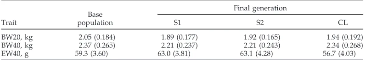
The 3 lines were analyzed separately. The 905 recorded hens of the base generation (1983) were, however, in-cluded in all 3 data sets, which thus comprised 3,935, 3,938, and 2,780 recorded hens, respectively. Two genera-tions of parents of the base generation without records were known and included in the analysis. The pedigree lists of the 3 lines contained 4,661, 4,665, and 3,506 animals for S1, S2, and CL, respectively. Three traits correlated to the complex selection criterion, i.e., income from eggs sold minus feed costs between 20 and 40 wk of age, were analyzed. These traits were BW at 20 and 40 wk of age and the average egg weight of this period (BW20, BW40, and EW40, respectively). Phenotypic means and standard deviations of these traits are given in Table 1 for the common base population and the final generation of the 2 selection lines (S1 and S2) and the control line (CL). The values show only slight phenotypic changes in BW but marked changes in egg weight. These traits are known to often follow a normal distribution rather closely and were, therefore, not transformed, e.g., as done by Szy-dłowski and Szwaczkowski (2001). The range of the skew-ness measure for the 3 traits was between 0.24 and 0.52, and the range of the kurtosis measure between 0.14 and 0.69. These values are similar or even considerably better than values given by Szydłowski and Szwaczkowski (2001) for traits transformed according to Box and Cox (1964). Results for traits with known strong deviations from a normal distribution will be presented elsewhere. More details on management of the birds and the repro-duction of the lines can be found in Hagger, (1990; 1992). A first attempt to search for a major locus of EW40 in this population was undertaken by Hagger and Stricker (1998) with several approximations to enable a likelihood method. Results from that approach, however, were in-conclusive.
Statistical Methods
The mixed inheritance model used contains a polygenic and a major locus effect (Janss et al., 1995). Two alleles are considered at the major locus, with genotypes A1A1, A1A2, and A2A2, with frequency f+ for the A2 allele (frequency of increasing allele) and 1− f+ for the A1 allele, and genetic effects according to Falconer (1982) of−a, d, and a, respectively, where a is called the additive effect and d the dominance effect. Using this kind of major locus model, dominance becomes estimable because genotypes are selected from a limited set of 3 possibilities only, unlike certain QTL models where effects are estimated for each haplotype or gamete (such as in Fernando and Grossman, 1989). The following linear model was fitted to the data of each line, one trait at a time:
TABLE 1. Phenotypic means (SD) of BW at 20 and 40 wk (BW20, BW40) and average egg weight to 40 wk (EW40) of base population and final generation of the 2 selected (S1 and S2), and control (CL) lines
Final generation Base Trait population S1 S2 CL BW20, kg 2.05 (0.184) 1.89 (0.177) 1.92 (0.165) 1.94 (0.192) BW40, kg 2.37 (0.265) 2.21 (0.237) 2.21 (0.243) 2.34 (0.268) EW40, g 59.3 (3.60) 63.0 (3.81) 63.1 (4.28) 56.7 (4.03) y = Xβ + Zu + ZWm + e
where y is the vector of individual records, β is a vector of fixed year of hatch effects, u is a random vector of polygenic effects, W is a 3-column matrix indicating with a 1 the possible genotype (A1A1, A1A2, or A2A2) at the major locus of an animal, m is the vector of the genetic effects at the major locus (i.e., –a, d, a), and e is the vector of random residuals. The X and Z are incidence matrices, connecting the unknowns in β, u, and Wm to the observa-tions. W is also an incidence matrix, but it is separated from Z because, firstly, it is unknown and has to be esti-mated in the statistical procedure, and, secondly, because W contains information on the genotypes of all animals in the pedigree, which is usually a larger set than the set of animals with records. Z is then used to connect genetic effects of the subset of animals with data to the appro-priate records. For u and e, normal distributions of the type N(0,Aσ2
a) and N(0,Iσ2e) were assumed, with A the
numerator relationship matrix and I the identity matrix of appropriate size. This animal model provides estimates for the parameters of the base population, i.e., all animals with unknown parents. The separate analysis of the 3 lines was thought justified, because propagation of a line was solely based on information of that line. Moreover, separate analysis of the 3 lines is interesting to validate the applied mixed inheritance model, because estimated parameters in the (common) base population are expected to be the same. Note, however, that small genetic differ-ences between the lines could have arisen from the assign-ment of the base generation females to the 3 lines and, later on, from selection and random drift.
The statistical procedure outlined by Janss et al. (1995) and implemented in a set of computer programs, called MAGGIC (Janss, 1998), were adapted and used for the investigations. The method constructs Monte Carlo chains of realizations of the model parameters through Gibbs sampling. These samples constitute the marginal posterior distributions of the model parameters, from which Bayesian inferences on these parameters can be drawn. In the programs of Janss (1998), blocked sampling of genotypes and of polygenic effects of a sire with its nonbreeder (final) progenies is used to improve conver-gence, and additionally a model-relaxation technique for the Mendelian sampling of alleles, as suggested by Shee-han and Thomas (1993), was used to further improve convergence of the Gibbs-chain to a steady state. Trial chains were run for each trait in each line to seek good relaxation parameters and for a suitable spacing between
samples to be kept, so that hopefully only independent samples were stored from the production chains. Five independent Gibbs-chains were then constructed for ev-ery line-trait combination and 100 samples kept from each chain, summing to a total of 500 samples. Locally uniform priors were assumed for the model parameters. A burn-in period of 5,000 cycles was completed before samples were kept in all chains.
For the post-Gibbs analysis of the samples, an ANOVA was used to check for equality of chains. This test also yields information about the dependency of the samples kept (Janss et al., 1997) within chain (convergence of chain). The marginal posterior means were used as esti-mators of the parameters. The highest posterior density regions (HPDR), according to Box and Tiao (1973), based on a nonparametric density estimate using the average shifted histogram method of Scott (1992), were deter-mined for all model parameters. The region is constructed in such a way that it includes the part 1-α of the probabil-ity mass about the smallest possible region of sampled parameter values. The HPDR guarantees that the density of each point within this region is equal or above the density of each point outside it. The HPDR allows, for example, the following reasoning: If the region for a vari-ance component or a frequency includes the boundary value of zero then this parameter is not of importance for this particular trait. In the present investigation, 1-α = 0.95 was used to construct the HPD95R. The posterior means of the frequencies of the 3 genotypes at the major locus (f1, f2, f3= 1-f1-f2), the values a, d, and f+, and the
derived additive genetic values α1and α2(Falconer, 1982)
were used to calculate the single locus variance compo-nents by the common variance formula. The total genetic variance is σ2g= [f1a2 + f2d2 + f3a2] − [f1(−a) + f2d + f3a]2.
Replacement of−a, d, and a in this formula by 2α1, α1+
α2, and 2α2yields σ2aand the difference σ2g− σ2ais σ2d. With
these quantities the total heritability, including the poly-genic and the major locus effects, amounts to h2
tot= (σ2p
+ σ2
a)/(σ2p + σ2a + σ2d + σ2e). The HPDR can also be
con-structed for the derived parameters. From each sample, the generation averages of the polygenic and the typic values as well as the average frequencies of 2 geno-types at the major locus (low homozygote and heterozygote) as well as the frequency of the A2 allele thereof (f++) were calculated for each year of hatch (gener-ation) and saved. These quantities should allow infer-ences about the genetic changes that occurred due to the selection applied, e.g., separation of the selection response
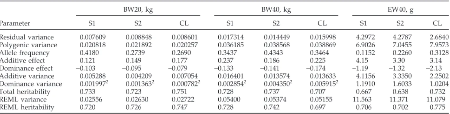
TABLE 2. Marginal posterior means of model and derived parameters for BW at 20 and 40 wk, and egg weight to 40 wk of the 2 selected (S1 and S2) and control (CL) lines and REML1estimates of genetic variance and heritability
BW20, kg BW40, kg EW40, g Parameter S1 S2 CL S1 S2 CL S1 S2 CL Residual variance 0.007609 0.008848 0.008601 0.017314 0.014449 0.015998 4.2972 4.2787 2.6840 Polygenic variance 0.020818 0.021892 0.020257 0.036185 0.038568 0.038869 6.9026 7.0455 7.9573 Allele frequency 0.4180 0.2739 0.2690 0.3437 0.4343 0.3464 0.1152 0.2260 0.3128 Additive effect 0.121 0.149 0.177 0.237 0.186 0.225 4.15 3.30 3.14 Dominance effect −0.103 −0.095 −0.079 −0.133 −0.141 −0.174 −1.19 −1.32 −2.13 Additive variance 0.005288 0.004209 0.007054 0.016401 0.013574 0.013633 4.1156 3.3350 2.2502 Dominance variance 0.0019972 0.0013632 0.0007822 0.0028542 0.0043502 0.0059152 1.1910 1.6033 1.0204 Total heritability 0.733 0.723 0.751 0.728 0.737 0.707 0.667 0.638 0.732 REML variance 0.02556 0.02630 0.02722 0.05400 0.05374 0.05155 11.563 11.371 11.079 REML heritability 0.720 0.726 0.747 0.728 0.742 0.697 0.706 0.702 0.775
1REML = Restricted maximum likelihood.
20.0 in 95% highest probability density region (HPD95R) included.
of a trait into the polygenic part and the part caused by the change of the allele frequency at the major locus. The selection response was calculated as the difference between the means of generations 1983 and 1990. The approach for a Bayesian analysis of selection experiments based on Gibbs sampling was outlined by Sorensen et al. (1994).
RESULTS AND DISCUSSION
Gibbs Sampling
Useful model relaxation factors for the 3 traits BW20, BW40, and EW40 varied between 0.0006 and 0.002. Relax-ation was speeding up the appearance of independent samples after initializing the Gibbs-chains. The frequency of the retained samples was further adjusted by the thin-ning rates, which had also been sought separately for each line-trait combination. On average, between 0.00847 and 0.0384% of all samples after the burn-in period were needed to get the 500 samples for each case. The ANOVA revealed that for all traits, 500 independent samples had been retained for each model parameter in all lines. The percentage of these samples was considerably smaller than the values reported by Janss et al. (1997) for meat quality traits in pigs, i.e., much longer Gibbs-chains were necessary.
Model Parameters, Allele Frequency,
and Genotypic Values
The estimates of the residual variances of BW20 and BW40 (Table 2) and the respective HPD95R (not shown) were rather similar between the lines. No systematic ten-dency between the selection lines and the control line were seen in the 2 BW traits. For EW40, however, the estimate of the residual variance was considerably smaller in the CL line than in S1 and S2 lines. The HPD95R, however, were not completely separate. The 2 most dis-joint regions with the upper bound of 3.50 of the leftist and a lower bound of 3.36 of the rightist region of the residual variances were between S1 and CL. The estimates
of the polygenic variances were also very similar between lines within BW20 and BW40 and so were the HPD95R. For EW40, estimates of this variance were smaller for the S1 and S2 lines than for the CL line. The corresponding HPD95R did, however, not support a difference at a 5% significance level. The opposite differences in the esti-mates for the 2 variance components between the selec-tion and the control lines led to a considerable difference in the estimates of the polygenic heritability (not shown). Again, the HPD95R did not support this difference. The estimated frequencies of the allele that caused the higher genotypic (f+) value at the major locus for BW20 and BW40 showed some differences between the lines. This appears to not be a systematic effect (Table 2), because one combination of S1 or S2 with CL was nearly identical in both cases. The boundary value of zero for this parame-ter was never within the HPD95R. The regions overlap and, thus, do not support the observed differences. A different situation appeared for the allele frequencies in EW40. The estimate for CL was nearly 3 times the value found for S1. This difference was supported by the corres-ponding HPD95R, where the upper limit from the left and the lower limit from the right region were 0.195 and 0.215, respectively.
The posterior means of the additive effects (estimates),
a, were sizable for BW20 and BW40 in all lines (Table 2).
The value of zero was always outside the left boundaries of the HPD95R and the 3 regions overlapped considerably between lines. The estimates of a for BW20 cannot be compared with the values given by Szydłowski and Szwaczkowski (2001), because these authors used a trans-formed BW. The estimates of the a effect for EW40 were between 3.1 and 4.2 g. The corresponding HPD95R were relatively narrow and their left boundaries were well to the right of zero. The 3 regions overlapped between the lines and thus did not support systematic differences be-tween them. Negative estimates for the dominance effect,
d, were obtained for BW20 and BW40. The value of zero
was never inside their HPD95R and the regions also over-lapped. The absolute size of d was always smaller than
a, therefore, pointing to a codominant inheritance mode
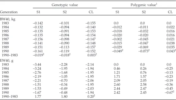
TABLE 3. Marginal posterior means of genotypic and polygenic values for BW at 40 wk (BW40) and egg weight to 40 wk (EW40) from the 2 selected (S1 and S2),
and the control (CL) lines, correlated genetic changes
Genotypic value Polygenic value1
Generation S1 S2 CL S1 S2 CL BW40, kg 1983 −0.142 −0.101 −0.155 0.0 0.0 0.0 1984 −0.132 −0.094 −0.140 −0.012 −0.011 0.022 1985 −0.135 −0.091 −0.153 −0.018 −0.032 0.016 1986 −0.135 −0.094 −0.154 −0.020 −0.020 0.016 1987 −0.156 −0.098 −0.147 −0.002 −0.045 0.021 1988 −0.141 −0.090 −0.148 −0.015 −0.047 0.038 1989 −0.151 −0.113 −0.157 −0.029 −0.069 0.035 1990 −0.161 −0.119 −0.152 −0.0492 −0.0732 0.0432 1990–1983 −0.0192 −0.0182 0.0032 EW40, g 1983 −3.44 −2.28 −2.14 0.0 0.0 0.0 1984 −3.24 −1.95 −1.94 0.46 0.26 −0.25 1985 −2.76 −1.68 −1.95 1.21 0.76 −0.13 1986 −2.19 −1.05 −1.95 1.71 1.57 −0.23 1987 −2.21 −0.70 −2.06 2.09 2.05 −0.19 1988 −1.51 −0.34 −1.95 2.60 2.58 −0.36 1989 −1.53 −0.49 −2.03 2.44 2.47 −0.45 1990 −1.67 −0.48 −1.94 2.42 2.45 −0.672 1990–1983 1.77 1.80 0.202
1Polygenic value of 1990 equals 1990–1983.
20.0 in 95% highest probability density region (HPD95R) included.
of a − |d| (= 0.0 for complete dominance, not shown), however, included zero in 4 out of 6 cases, which suggests that the degree of the dominance inheritance was unclear. Negative dominance effects resulted also for EW40 (Table 2). For this trait, the right boundaries of the HPD95R were always to the left of zero and the corresponding region of|d| included zero for CL only. The degree of dominance was, therefore, not clearcut for this trait. The observed differences between the estimates of the lines were not supported by the HPD95R.
Derived Parameters
The σ2
aand σ2d variances due to the major locus were
calculated from the estimates of the model parameters as shown above. The polygenic variance turned out to be 3 to 4 times the size of σ2a for BW20 and 2 to 3 times that
size for BW40. The σ2
d values were much smaller than
the σ2
a values for the BW traits. The HPD95R of σ2d for
BW20 and BW40 included zero in all lines. Polygenic and major locus variance components resulted in h2tot of
around 0.73 and were close to the restricted maximum likelihood (REML) estimates from the conventional ani-mal model (Table 2). The HPD95R of the h2totfor the 3
lines were very close to each other. For EW40, σ2 a was
between 0.3 and 0.6 σ2
pol. This parameter showed
consider-able differences between the lines. A low allele frequency was connected with a high variance and vice versa. The HPD95R showed large overlapping between the lines. The σ2
d values were also smaller in this trait than the σ2a
in all lines. The corresponding HPD95R did not include zero in all cases. The smaller residual and larger polygenic variances resulted in a higher h2
tot for EW40 in CL in
spite of smaller σ2
a compared with S1 and S2 (Table 2).
The HPD95R of the lines overlapped and, thus, did not support systematic differences between these herita-bilities.
The sums σ2pol+ σ2a, i.e., the genetic variance usable for
selection, for the 2 BW traits were almost identical to the estimates of σ2
aREML. This was in contrast to EW40 where
σ2aREMLwas distinctly larger than the sum of the 2
compo-nents just mentioned. This observation coincided with the importance of σ2din these traits. The HPD95R for this
component include zero for all BW cases, whereas for EW40, these regions are well to the right of zero. The REML estimates for the heritability of BW20 and BW40 were almost identical to the posterior means of the h2
tot
from the mixed inheritance model. For EW40, with a significant dominance component, the REML estimate of this parameter was, however, clearly above the h2
tot of
the mixed inheritance model.
Correlated Selection Responses
for Polygenic and Genotypic Values,
and Allele and Genotype Frequencies
Correlated selection responses in BW20 were at most very small in all lines and will not be discussed. Genera-tion averages (marginal posterior means) of major locus and polygenic values, which are a way to express selec-tion responses, are given in Tables 3 and 4 for BW40 and EW40. Slight negative trends were observed for both genetic values of BW40 in the S1 and S2 lines (Table 3). The differences between years 1983 and 1990 (correlated selection responses) amounted to−19 and −18 g for the genotypic, and to−49 and −73 g for the polygenic values
TABLE 4. Marginal posterior means of the frequencies of the positive allele (f++),1the low homozygote
(hom), and the heterozygote (het) genotypes at the major locus for BW at 40 wk (BW40) and egg weight to 40 wk EW40 of the selected (S1 and S2), and the control (CL) lines, correlated genetic changes
S1 S2 CL
Generation f++ hom het f++ hom het f++ hom het
BW40 1983 0.316 0.438 0.459 0.410 0.331 0.499 0.322 0.432 0.463 1984 0.342 0.401 0.480 0.426 0.289 0.528 0.367 0.390 0.473 1985 0.340 0.427 0.455 0.438 0.299 0.508 0.329 0.432 0.458 1986 0.341 0.430 0.452 0.432 0.303 0.509 0.328 0.441 0.450 1987 0.260 0.452 0.477 0.418 0.328 0.496 0.353 0.436 0.438 1988 0.324 0.442 0.450 0.446 0.326 0.473 0.347 0.434 0.444 1989 0.300 0.486 0.421 0.366 0.346 0.518 0.319 0.454 0.443 1990 0.268 0.517 0.409 0.345 0.385 0.494 0.334 0.436 0.451 1990–1983 −0.0492 0.0792 −0.0502 −0.0642 0.0532 −0.0052 0.0122 0.0042 −0.0112 EW40 1983 0.132 0.776 0.205 0.225 0.588 0.359 0.294 0.459 0.452 1984 0.122 0.710 0.272 0.280 0.493 0.424 0.348 0.438 0.439 1985 0.217 0.607 0.343 0.337 0.437 0.445 0.343 0.443 0.437 1986 0.303 0.497 0.410 0.434 0.295 0.512 0.347 0.456 0.422 1987 0.237 0.447 0.492 0.484 0.232 0.529 0.307 0.428 0.474 1988 0.372 0.360 0.498 0.542 0.188 0.514 0.342 0.435 0.444 1989 0.391 0.391 0.453 0.516 0.199 0.531 0.317 0.440 0.456 1990 0.340 0.377 0.502 0.524 0.215 0.507 0.345 0.444 0.433 1990–1983 0.208 −0.399 0.297 0.298 −0.373 0.1492 0.0502 −0.0152 −0.0192 1Calculated from genotypic frequencies.
20.0 in 95% highest probability density region (HPD95R) of genetic changes included.
in the 2 lines. All corresponding HPD95R included zero and, therefore, no significance of systematic trends can be postulated for the 2 genetic parts of this trait. The same conclusion resulted for the total correlated response (sum of the 2 parts) in both selection lines (not shown). A negative genetic trend could be expected from selection for income minus feed cost in laying hens, because a lower BW would mean a lower feed intake due to a lower maintenance requirement. The observed changes were not very large, although in the right direction. No genetic change in BW was observed in the CL line, where the polygenic change was positive and thus contrary to the S1 and S2 lines, but zero was also included in the HPD95R. The higher genotypic value in the S2 line right from the beginning of the experiment was a consequence of the higher frequency of the major locus allele increasing BW40, f+ in Table 2. This was also expressed in the esti-mated frequencies of the low homozygote and the hetero-zygote genotypes in Table 4. A slight increase of this homozygous genotype was seen in both selection lines, which, of course, was identical to the series of genotypic values. Both differences were direct consequences of the difference in allele frequency between the 2 lines. The HPD95R for the allele frequencies did not, however, sup-port a systematic difference between all the lines concern-ing the major locus contribution to the correlated selection responses in BW40.
The negative genotypic values for EW40 in all lines (Table 3) were the consequence of the low posterior means of the frequency of the positive allele at the major locus (f+), particularly in the 2 selected lines. Income from eggs sold, as used in the selection criterion, was strongly de-pendent on egg weight (Hagger, 1990). Selection for in-come minus feed cost led, therefore, to a correlated
increase in average genotypic values of 1.81 and 1.80 g in this trait over 7 generations of the experiment in the S1 and S2 lines, respectively. The restriction of no genetic change in egg weight, included in the selection criterion of the last 2 generations, was not clearly expressed in the genotypic values of the affected generations. For the polygenic values, an increase of 2.45 g in the S1 and S2 lines was observed during the experiment. The restriction of no genetic change in egg weight was clearly expressed in the corresponding generation averages of the polygenic values (Table 3). It should be noted that the selection criterion was based on the purely infinitesimal model. The HPD95R of the 2 genetic parts as well as for the total response were well to the right of zero. The regions overlapped strongly between the 2 selection lines and, thus, confirm the visible similarity. The HPD95R of the CL line for the changes of genotypic and polygenic changes contained zero, though systematic changes were not sup-ported. The differences between the genotypic and poly-genic responses were not supported by their HPD95R in all lines.
The frequencies of the low homozygote and the hetero-zygote genotypes of the major locus for EW40 reflect the posterior means of the allele frequencies, f++, in all lines (Table 4). Selection for income minus feed cost favored high egg weight and, therefore, led to an increase of the positive allele, which, as a consequence, diminished the frequency of the low homozygote and increased the het-erozygous and high homozygous (not shown) genotypes in the S1 and S2 lines. From the HPD95R for the changes in genotypic frequencies from 1983 to 1990 only the region for the heterozygote in the S2 line contained zero. The very small changes of the genotypic frequencies during
the experiment in the CL line were supported by their HPD95R, both of which included zero.
The Bayesian approach of Janss et al. (1995) was found to be very useful for fitting a mixed inheritance model to data from a selection experiment with laying hens (Hagger, 1992). The procedure applies Gibbs sampling with blocked sampling of genotypes and relaxation of the transmission constraints (Sheehan and Thomas, 1993) for simulating genotypes of the major locus. Preliminary test runs were necessary to obtain reference points for the relaxation parameter and the thinning rate for the samples to be kept. These quantities determine the computing time to obtain the desired number of chains, and the number of independent samples required per chain, i.e., 5 chains of 100 samples each in this investigation. The attempt worked well for most trait (BW20, BW40, and EW40) and line (S1, S2, and CL) combinations. In some cases, the 2 parameters had to be retuned to get the at-tempted 500 independent samples from 5 chains. No sys-tematic reason was observed for this behavior. Janss et al. (1997) reported a similar observation, which was as-signed to traits. For a trait not shown here, the post-Gibbs analysis revealed that 300 independent samples had been obtained from the first 3 chains. After adding the 100 samples from one additional chain, the number of inde-pendent samples declined strongly for most model pa-rameters. This might be an indication that the number of independent samples taken should be large enough to avoid such situations.
The 3 lines (S1, S2, and CL) of the experiment can genetically be viewed as samples from one base popula-tion. The marginal posterior means obtained of one partic-ular trait of the mixed inheritance model to each line are, therefore, estimates of the base population parameter for this trait. This assumption was supported by the observed overlapping of the corresponding HPD95R between the lines, with the only exception being the regions for the allele frequency of EW40 for the S1 and CL lines. It seems, therefore, that the procedure of Janss et al. (1995) did estimate the parameters (posterior means) of the base population rather well in spite of the selection applied over 7 generations in the S1 and S2 lines. Hence, this full-pedigree segregation analysis appeared to work well in a multigeneration analysis and appeared to handle well selection on the analyzed trait. Furthermore, it seems that from the model parameters allele frequency, residual variance, and, to some extent, the dominance effect were more sensitive to selection effects (larger differences be-tween marginal posterior means) than the polygenic vari-ance and the additive effects. Some consequences of these circumstances appear in the derived parameters. The re-sults from the mixed inheritance model suggested a co-dominant mode of inheritance at the major locus for the 3 traits. The allele causing lower trait values was always the dominant one. The degree of dominance was not clearcut, although complete dominance could sometimes not be rejected.
Scaling the effects of major loci is necessary to make useful comparisons between traits, populations, or even
species. It is often done to one of the population variances or standard deviations. The major loci found here ex-plained 19.7 to 43.6% of the total genetic variance. The substitution effects (a-value) were between 0.75 and 1.25 genetic standard deviations, or from 0.64 to 1.02 pheno-typic standard deviations. Compared with a QTL, i.e., an estimated effect due to a genetic marker, the major loci found here were of relatively modest size. Van Kaam et al. (1998) performed a whole genome scan to detect QTL affecting BW in broilers and identified one significant QTL with a substitution effect of 1.2 genetic standard deviations. Hayes and Goddard (2001), in a meta-analysis of mapping experiments, found a raw average QTL effect expressed in phenotypic standard deviations of 0.42 for pigs and of 0.32 for dairy cattle. These values are below the values found in the present study. It should be noted that mapping experiments in dairy cattle are (due to their large and selected data sets) the most powerful ones to-day, and that pig experiments were established by cross-ing breeds with large phenotypic differences to increase power. Thus, it is not too surprising that the relative genetic effects found here as well as the one from the broiler experiment mentioned were larger than the corres-ponding average effects of the other 2 species.
Although the contributions of the major loci to the whole genetic influence were sizable, the REML and the mixed inheritance model estimates for the usable genetic variances and heritabilities were very similar, especially for the BW traits. This indicates that the conventional quantitative genetic model takes up the additive variance of a major locus and suggests that the same response from selection according to either model could be expected. However, it might be that selection on a combination of the 2 genetic parts would increase the rate of response at the early stage of such a scheme compared with conven-tional selection.
The detection of a relatively modest major locus con-firms that this type of analysis with data from selected lines was indeed powerful. A previous analysis by Hag-ger and Stricker (1998) remained inconclusive, probably because intensive cutting of pedigree loops, which was required to allow a likelihood-based approach, destroyed too much information about the underlying selection process.
The allele frequencies (Table 4) were calculated from the genotype frequencies, assuming Hardy-Weinberg proportions within generation. The estimates for year 1983, which was the first recorded, were in most cases very similar to the base population estimates (f+ in Table 2). For BW40, the HPD95R of the change in allele fre-quency from 1983 to 1990 included zero not only in the control, but also in the selected lines. This observation was in agreement with the low genetic correlation found by a REML analysis between the selection criterion and BW40 of−0.16 for the whole population (Hagger, 1992). In EW40, the allele frequency changed considerably in the S1 and S2 lines over the duration of the experiment. This was suggested by the high genetic correlation be-tween the selection criterion and EW40 of 0.53 (Hagger,
1992). The HPD95R were well to the right of zero. In the CL line, this change was small and the corresponding HPD95R included zero. The results show further that the CL line remained genetically stable over the duration of the experiment. The observed changes were not sup-ported by the HPD95R in both traits. It may be that the steady decrease of the polygenic value in EW40 in the CL line since generation 1987 (Table 3) is an indication of a systematic change, which could become significant after a few additional generations. The question of whether the major loci detected for BW20 and BW40 are identical was not investigated.
REFERENCES
Box, G. E. P., and D. R. Cox. 1964. An analysis of transformations. J. R. Stat. Soc. [Ser. B] 26:211–243.
Box, G. E. P., and G. C. Tiao. 1973. Bayesian Inference in Statisti-cal Analysis, Addison-Wesley, Boston.
Elston, R. C., and J. Stewart. 1971. A general model for the genetic analysis of pedigree data. Hum. Hered. 21:523–542. Falconer, D. S. 1982. Introduction to Quantitative Genetics. 2nd
ed. Longman, London.
Fernando, R. L., and M. Grossman. 1989. Marker-assisted selec-tion using best linear unbiased predicselec-tion. Genet. Sel. Evol. 21:467–477.
Gowe, R. S., A. Robertson, and B. D. H. Latter. 1959. Environ-ment and poultry breeding problems. 5. The design of poul-try control strains. Poult. Sci. 38:462–471.
Hagger, C. 1990. Responses from selection for income minus food cost in laying hens, estimated via the animal model. Br. Poult. Sci. 31:701–713.
Hagger, C. 1992. Two generations of selection on restricted Best Linear Unbiased Prediction breeding values for income mi-nus feed cost in laying hens. J. Anim. Sci. 70:2045–2052. Hagger, C., and C. Stricker. 1998. Infinitesimal and segregation
analyses of a trait under selection. Proceedings of the 6th World Congress on Genetics Applied to Livestock Produc-tion, Armidale, Australia 26:37–40.
Hayes, B., and M. E. Goddard. 2001. The distribution of the effects of genes affecting quantitative traits in livestock. Genet. Sel. Evol. 33:209–229.
Ilahi, H., and H. N. Kadarmideen. 2004. Bayesian segregation analysis of milk flow in Swiss dairy cattle using Gibbs sam-pling. Genet. Sel. Evol. 36:563–576.
Janss, L. L. G. 1998. Manual and Documentation with maGGic 4.0. Agric. Res. Dept., ID-DLO Lelystad, The Netherlands. Janss, L. L. G., R. Thompson, and J. A. M. Van Arendonk. 1995.
Application of Gibbs sampling for inference in a mixed major gene-polygenic inheritance model for animal populations. Theor. Appl. Genet. 91:1137–1147.
Janss, L. L. G., J. A. M. Van Arendonk, and E. W. Brascamp. 1997. Bayesian statistical analyses for presence of single genes affecting meat quality traits in a crossbred pig population. Genetics 145:395–408.
Ma¨ki, K., A. F. Groen, L. L. G. Janss, A. E. Liinamo, and M. Ojala. 2002. Segregation analysis for hip and elbow dysplasia in the Finnish Rottweiler. Communication 13–14 in 7th World Congress on Genetics Applied to Livestock Production, Mon-tpellier, France.
Miyake, T., T. Dogo, K. Moriya, and Y. Sasaki. 1999. Bayesian analysis for existence of segregation of major genes affecting carcass traits in Japanese Black cattle population. J. Anim. Breed. Genet. 116:207–215.
Navarro, P., A. N. M. Koerhuis, D. Chatziplis, P. M. Visscher, and C. S. Haley. 2002. Genetic studies of ascites in a broiler population. Communication 04–14 in 7th World Congress on Genetics Applied to Livestock Production, Montpellier, France.
Scott, D. W. 1992. Multivariate Density Estimation: Theory, Prac-tice, and Visualization. John Wiley, Inc., New York. Sheehan, N., and A. Thomas. 1993. On the irreducibility of a
Markov chain defined on a space of genotype configurations by a sampling scheme. Biometrics 49:163–175.
Sorensen, D. A., C. S. Wang, J. Jensen, and D. Gianola. 1994. Bayesian analysis of genetic change due to selection using Gibbs sampling. Genet. Sel. Evol. 26:333–360.
Szydłowski, M., and T. Szwaczkowski. 2001. Bayesian segrega-tion analysis of producsegrega-tion traits in two strains of laying hens. Poult. Sci. 80:125–131.
Van Kaam, J. B. C. H. M., J. A. M. van Arendonk, M. A. M. Groenen, H. Bovenhuis, A. L. J. Vereijken, R. P. M. A. Crooij-mans, J. J. van der Poel, and A. Veenendaal. 1998. Whole genome scan for quantitative trait loci affecting body weight in chickens using a three-generation design. Livest. Prod. Sci. 54:133–150.