HAL Id: hal-01107479
https://hal.archives-ouvertes.fr/hal-01107479
To cite this version:
Mena B. Lafkioui. DIALECTOMETRY ANALYSES OF BERBER LEXIS. Folia Orientalia, Zaklad Narodowy im. Ossolińskich, Oddzial w Krakowie, 2008, 44, pp.71 - 88. �hal-01107479�
DIALECTOMETRY ANALYSES OF BERBER LEXIS1
Mena Lafkioui
Università di Milano-Bicocca – Ghent University
1. Introduction to methods in dialectometry
Dialectometry is a quantitative methodology for calculating linguistic distances between linguistic varieties. The most frequently used dialectometry methods can be divided into the categories of traditional and computational methods.2
The most well-known traditional approaches are those based on the concept of isogloss, which is a line that bisects a geographic map into separate zones according to the detected linguistic features. The classification of the varieties is deducted from the arrangement of isoglosses, clusters of isoglosses (Goossens 1969) or clusters of demarcative isoglosses (Stankiewicz 1957; Garde 1961; Lafkioui forthcoming 2) on the geolinguistic map.3 Although this method allows for verification of the visualised facts, it has several disadvantages, including the difficulty to find clusters of isoglosses that precisely divide the geolinguistic area examined (Kessler 1995; Chambers & Trudgill 1998).4
Another traditional technique is the geolinguistic structuring method which divides a geographic area depending on the linguistic structure of its varieties (Moulton 1960; Goossens 1965, among others). For instance, varieties with the same phonemic system are part of the same geolinguistic group. However, classifications based on this method are mainly
1 This article reflects, in large part, the content of Lafkioui (forthcoming 3).
2 There also exist different perceptual approaches that permit to draw sociolinguistic
borders based on the speaker’s “dialectal conscience” (Weijnen 1946, 1966; Rensink 1955; Daan & Blok 1969; Gooskens 1997, 2002; among others).
3 The qualifying term “demarcative”, added to the common dialectology criterion of
“isogloss clusters” (Goossens: 1969, 54), refers to the structural value of the isoglosses relating to the material aspect of the phenomena as well as to their relative distribution (direction and density). Thus, not only the quantitative dimension (number) of isoglosses is relevant to the typology of classification, but also the qualitative aspect, i.e. their degree of importance. However, non-demarcative isoglosses may also be of great significance for the classification, especially when they allow an evaluation of the results. On the relationship between “structuralism” and “dialectology”, see Forquet (1956), Weinreich (1954), Grosse (1960) and Martinet (1972), among others.
4 A significant critique on this method is that it cannot completely exclude some
subjectivity because isoglosses might be chosen, a priori, according to the linguistic borders they yield (Goossens 1977).
phonological and therefore lack an interpretation basis that is connected to other linguistic dimensions.5
The computational dialectometry methods are numerous and are currently considered most adequate for reasons I will explain later on in this article. The foundations of digital automated dialectometry were established by Séguy (1973) with his analytical method to calculate the linguistic differences between varieties of Gascogne. The comparison is based on an algorithm which classifies data as identical or non-identical. The sum of the measured distances between two varieties matches their linguistic distance. The visualisation of the classification analysis is conducted through lines of various types (bold/non bold, dotted/non dotted, etc.), which divide the region according to the linguistic differences of the varieties. As a counterpart, Goeble (1982, 1993) has calculated the similarities between varieties from Italy and Southern Switzerland. Even though the results of the calculation of Séguy and Goeble have the merit of being objective, they lack refinement because their technique excludes distance graduation.
The main computational methods based on the frequency of linguistic variants are the “Corpus Frequency Method” (Hoppenbrouwers & Hoppenbrouwers 1988, 2001) and the “Frequency per Word Method” (Nerbonne & Heeringa 1998, 2001). The basic principle of the first approach is that the degree of difference/similarity between two varieties is derived from comparing the frequency of the marked linguistic features of their variants. The problem in this approach is that the entity “word” is not considered as a linguistic unit. However, this obstacle is removed by the second approach which assigns to words the status of “units” functioning as such. Nevertheless, the two classification tools do not take into account the order of the phonic units in the sequence.
The “Levenshtein distance” (Lv), on the other hand, allows incorporating the parameter of sequential ordering of phonic units in the classification, which makes it more appropriate than other digital/numerical methods. This tool has been introduced in dialectometry by Kessler (1995), who has applied it to a corpus of Irish Gaelic. The Levenshtein distance measure
the phonic units: the pair [t, d] has the same cost as the pair [u, t] and [u, u:]. Yet, with the technique of “feature string comparison” phonetic features of phonic units can be compared: the cost of the pairs [u, t] and [u, u:] is not equal because the phonetic affinity between the phonic units of [u, u:] is greater than that of [u, t].
2. Dialectometry analyses of Berber lexis
Among the different existing dialectometry approaches, I prefer the computational methods because they allow handling large data corpora with certain ease, while ensuring the accuracy and consistency of the analyses. These aims can be achieved thanks to the fact that
− Distances and frequencies are measured automatically. − Data are classified digitally.
− Mapping can be assisted by the computer.
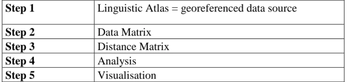
− Statistical analyses can be made and displayed automatically. The dialectometry analyses that I present in this article were performed with the free software of Kleiweg (RuG/L04).6 In order to complete a displayed dialectometry analysis, all the procedural steps summarised below are indispensable (Lafkioui forthcoming 1):
Table 1: General procedure of computational dialectometry analysis
Step 1 Linguistic Atlas = georeferenced data source
Step 2 Data Matrix
Step 3 Distance Matrix
Step 4 Analysis
Step 5 Visualisation
2.1. The Linguistic Atlas of the Rif as a data source
The Rif is that region of North Morocco stretching from the Strait of Gibraltar in the West to the Algerian frontier in the East. The Rif-Berber varieties (Tarifit) belong to the northern Berber languages and thus are part of the large Afro-Asiatic language phylum. The Berber-speaking area of the Rif is delimited:
- In the West, by the varieties of the Ktama tribe, (the so-called Senhaja varieties).
- In the South, by the koinè of Gersif, which is the ultimate geographic point where Rif-Berber (Tarifit) is spoken before reaching the corridor of Taza.
- In the East, by the varieties of Iznasen, which have spread to the regions of Arabic speaking varieties to the Morocco-Algerian border.
The lexical data which are compared and classified in this study are collected from the Atlas linguistique des variétés berbères du Rif (Lafkioui 2007) or ALR. The digital data corpus consists of sixty-two lexemes regarding the human body (maps 295 to 315), kinship (maps 316 to 321 cards), animals (maps 322 to 327), colours (maps 328 and 329), numbers (maps 330 to 332), besides a subset of various nouns and verbs (maps 333 to 356). Of these lexemes, eleven have only one variant per variety; all fifty-one other lexemes display the co-occurrence of multiple variants for each lexeme.
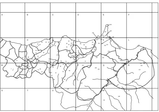
Due to the completion of the automated ALR, the data obtained from it are already in digital format, which has avoided a great task of digitising. However, an adaptive conversion to the software RuG/L04 (Kleiweg) was necessary. The ALR also offers a precise digital map of the Rif region (see Figure 1), which is essential to the visualisation of the dialectometry analyses, except for the dendrogram.
Figure 1: Map of the georeferenced survey points of the Rif (Lafkioui 2007) 78 77 130 124 133 136 A G M S B H N T C I O U D J P V E K Q W F L R X 102 109 96 7 98 113 2 108 8 23 105 107 13 26 115 11 68 70 114112111 138 62 65 69 100 110 42 104 106 71 40 134 29 66 30 117 72 81 52 121 116 43 45 3735 5954 119 73 131 32 31 39 3634 61 60 55 38 56 120 126 50 125 137 16 18 17 33 3 1 4 5 9 12 14 10 19 27 28 22 25 24 92 88 95 89 87 93 90 94 91 44 41 49 46 47 48 67 64 63 75 76 79 74 53 51 58 57 86 80 103 99 97 101 6 20 135 127 128 129 85 83 84 141 139 140 132 122 123 118 82 21 15
One hundred forty-one georeferenced points – belonging to thirty-two Rif tribes – were selected from a group of four hundred fifty-two localities in the Rif according to their degree of linguistic variation (Lafkioui 2007).7
7 The survey points were selected on the basis of the principle of equidistance dividing the
inquiry field into several grids to which were assigned points that could match with localities on the field. The greater the variation was, the more the grids were reduced. The four hundred fifty-two locations selected for this research were for the most part chosen so that they could, a priori, indicate linguistic borders. This selection mainly stemmed from the scientific and empirical knowledge of the investigator on the different varieties spoken in the Rif area.
2.2. Data matrix of Rif-Berber lexis
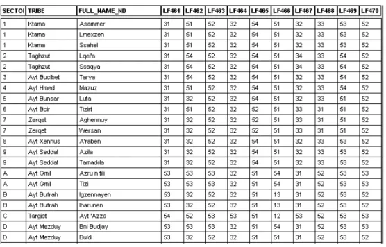
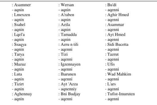
The data matrix is composed of digital lexical excerpts from the ALR (Lafkioui 2007) converted following the format of the software RuG/L04 (Kleiweg). Here below, a small sample in digital format of the ALR (Mapinfo Professional format; Table 2) and in text format of RuG/L04 (Table 3) are given:
Table 3: Data excerpt in text format of RuG/L04 : Asammer - aqnin : Lmexzen - aqnin : Ssahel - aqnin : Lqel'a - aqnin : Ssaqya - aqnin : Tarya - aqnin : Mazuz - aqnin : Luta - aqnin : Tizirt - aqnin : Aghennuy - aqnin : Wersan - aqnin : A'raben - aqnin : Azila - aqnin : Tamadda - aqnin : Azru n tili - aqenni : Tizi - aqenni : Igzennayen - aqenni : Iharunen - aqenni : Ayt 'Azza - aqnenniy : Bni Budjay - aqenni : Bu'di - aqenni : Aghir Hmed - aqenni : Asammar - aqenni : Ayt Hmed - aqenni : Sidi Bucetta - aqenni : Tazrut - aqenni : Ufis - aqenni : Wad Mahkim - aqenni : L'ars - aqenni : Tufist-Imuruten - aqenni
2.3. Distance matrix of Rif-Berber lexis
This section contrasts the three most employed digital comparison techniques: the Binary distance (Hamming algorithm), the Gewichteter Identitätswert distance (Weighted identity value), and the Levenshtein distance. I will apply these techniques on the Rif-Berber lexical corpus to test their validity and to select the most appropriate to Berber. Each distance measuring allows acquiring precise numerical values derived from the linguistic comparison between the varieties of the Rif area. These values make up the distance matrices (symmetric matrices N x N, N= sum of varieties), whose configuration differs depending on the adopted algorithm.
2.3.1. Binary distance
The Binary distance (Bin) is used to classify lexical units as being identical or non-identical: comparison of type 0-1; 0= resemblance and 1= difference. Table 4 presents an excerpt from the Binary distance matrix of the lexeme "heel" (ALR, map 312):
Table 4: Excerpt from the Binary distance matrix of the lexeme "heel"
2.3.2. Gewichteter Identitätswert distance
The Gewichteter Identitätswert distance (GIW) deviates from the Binary distance in that the frequency of the lexical variants is considered in the comparison: low-frequency variants weigh heavier than high-frequency variants. The distance obtained by this technique varies between 0 and 1; {0
≤ d ≤ 1}. Table 5 presents an extract from the distance matrix of the lexeme “heel”:
2.3.3. Levenshtein distance
The distance values resulting from a Levenshtein-based comparison – an algorithm taking into account the sequential order of phonic units composing lexemes – fluctuate between 0 and 1, {0 ≤ d ≤ 1}, as shown in the following excerpt:
Table 6: Excerpt from the Lv distance matrix of the lexeme “heel”
These values result from the selection of the least costly calculation to transform a lexical unit – as a string of phonic units – into another. Table 7 depicts the lowest cost of operations which allow modifying the string
awrez (heel) into inerz (heel):
Table 7: Cost of operations allowing modification of awrez into inerz (heel)
a w r e z 0 0.5 1 1.5 2 2.5 i 0.5 1 1.5 2 2.5 3 n 1 1.5 2 2.5 3 3.5 e 1.5 2 2.5 3 2.5 3 r 2 2.5 3 2.5 3 3.5 z 2.5 3 3.5 3 3.5 3
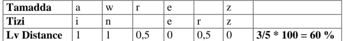
The lowest cost of operations amending awrez into inerz is 3, which implies that the distance between these two lexemes is 3/5 (5 being the total number of features); consequently, the Levenshtein distance is 60%. These
calculations are based on operations that cost 0.5 for an insertion or deletion and 1 for a substitution. Table 8 illustrates this calculation technique:
Table 8 : Example of calculation of Lv distance for modifying awrez into inerz (heel)
Tamadda a w r e z
Tizi i n e r z
Lv Distance 1 1 0,5 0 0,5 0 3/5 * 100 = 60 %
2.4. Numerical dialectometry analyses of Rif-Berber lexis
From the distance matrices, numerical comparative analyses of Berber lexis can be accomplished through two techniques: Cluster Analysis and
Multidimensional scaling. The technique of Cluster Analysis (CA) consists
of regrouping data by reducing the distance matrix by means of various algorithms. According to Kleiweg (RuG/L04), I have implemented the Ward algorithm (minimum variance), which is generally regarded as one of the most appropriate algorithms for this type of analysis. On the other hand, multidimensional scaling (MDS) is:
“[…] a technique that, using a table of differences, tries to position a set of elements into some space, such that the relative distances in that space between all elements corresponds as close as possible to those in the table of differences.” (Kleiweg, RuG/L04).
2.5. Visualisation of dialectometry analyses of Rif-Berber lexis
Classification by clustering (CA) necessarily uses a dendrogram for its display. A dendrogram is a complex ranking structure, usually in colour, whose branches represent the linguistic varieties. It can be matched with a digital map, resulting in a geolinguistic map that shows the distribution of linguistic varieties depending on the linguistic differences and the selected classification criteria. In contrast, analyses by Multidimensional Scaling (MDS) directly offer maps on which the relative linguistic variation is
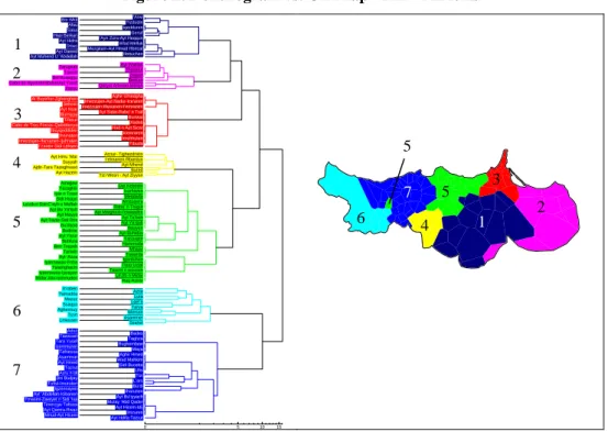
groups 6 and 7 and the major subgroup containing groups 1 to 5; the distance between these two subgroups is 16.17. This distance value indicates a relatively high linguistic boundary after group 7, which is delimited on the right by the varieties of Ayt Weryaghel and Ayt ‘Ammart. The major subgroup shows a rather balanced subdivision (d = 9.34) between groups 4 and 5 (variety of Targist included) and groups 1 to 3, which have also been subdivided. The second important linguistic border therefore coincides with the bordering varieties of groups 4 (Igzennayen) and 5 (Ayt S’id and Ayt Tuzin).
Figure 2: Dendrogram vs. CA Map - Bin – All lexis
’Arwi Bni WkilAfsu Tizdudin Iqedduren Saka
Gersif Hasi Berkan ’Ayn Zura-Ayt Heqqun Ayt Hidra Wlad Melluk Driwc Mezgitam-Ayt Hmed Hbircat Ayt Dawed
Ifettuchen Ayt Muhend U ’Abdellah
Ayt Waklan Tafughalt Thgasrut Tawrirt Zegzel Bni Buzeggu
Berkan Cabo de Agua-Imrabden/Ayt Yusef
Qaryat Arkman-Mellah Zayyu
Aghir Umedgha At Buyefrur-ZghenghenSelwan Imezzujen-Ayt Nadur-Ice’aren Imezzujen-Ifarxanen-I’emranen Ayt Nsar
Ayt Sidar-Rabe’ n Trat Bumiyya Burtwal Tifasur Xadeb Cabo de Tres Forcas-QabddenyaIbuyqeddiden Had n Ayt Sicar Icemraren Ihninaten Imehhuten Imezzujen-Ifarxanen-Ijuhraten Tibuda I’zanen-Sidi Lehsen Acnur- Tighezdratin Ayt Hmu ’Mar
I’etmanen-Rbardun Suyyah
Ayt Mhend Ajdir-Tara Tazeghwaxt Bured Ayt Hazem Tizi Wesri - Ayt Ziyyan
Amejjaw Dar Kebdani Tazaghin Isarhiwen Iyar n Tzaxt Meqdada Sidi Hsayn Amzzawru La’zib n Sidi C’ayb u Meftah Raba’ n Trugut Ayt Bu Ya’kubAyt Mayyit Ayt Marghnin-I’ewwaden Ayt Ta’ban Ayt Tayar-Sidi Dris
Ayt Ya’qub Bu’diyya Ifasiyen Budinar Ayt Buhidus Ayt YarurBuhfura Yarzuqen Hammuda Ben Teyyeb
Mhajar Tariwin Tawarda Ayt ’Azza Igarduhen Iyarmawas-FrihaTalamghacht Tlata Uzlaf Tawrirt n wuccen Iyarmawas-Ijarayen
La’zib n Midar Midar Alto-Icennuden Raq Azirar A’raben Azila Tamadda Luta Mazuz Lqel’a Ssaqya Tarya Aghennuy Wersan Tizirt Asammer Lmexzen Ssahel Aduz Bades Tawssart Taghza Tara Yusef Bughembew Izemmuren
Maya Tafnessa
Aghir Hmed Asammar Wad Mahkim Ayt Hmed Sidi Bucetta Tazrut Ufis Azru n tili Tizi Bni Budjay L’ars Tufist-Imuruten Bu’di Igzennayen Iharunen Ayt ’Abdellah-Icibanen Ayt Bu’iyyach Tmasint-Zawiyet n Sidi ’IsaTimerzga-Tafsast Mulay ’Abd Qader Ayt Hicem-Idij Ayt Qamra-Rwaz
Imzuren Mnud-Ayt Hicem Ayt Hdifa-Tazrut
0 5 10 15
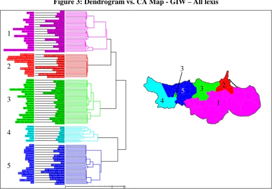
The classification based on the GIW algorithm diverges considerably from that based on the Bin algorithm, because it leads to a set of five clusters (Figure 3), of which cluster 1 includes the sub-clusters 1, 2 and 4 of the Bin classification (Figure 2). However, the main linguistic boundary detected through GIW – boundary drawn after the varieties of cluster 5 – is identical to the one that emerged from the Bin dendrogram. Although, the distance between the two major sub-clusters is lower for GIW (dGIW = 10.87) than for Bin (dBin = 16.17). This difference can be explained by the integration of the frequency parameter in the comparison.
1 2 3 4 5 6 7 6 1 7 4 2 5 3 5
Figure 3: Dendrogram vs. CA Map - GIW – All lexis
’Arwi Bni Wkil Tizdudin Afsu Iqedduren Saka
Gersif Hasi Berkan
’Ayn Zura-Ayt Heqqun Ayt Hidra Wlad Melluk Driwc Mezgitam-Ayt Hmed Hbircat Ayt Dawed
Ifettuchen Ayt Muhend U ’Abdellah Acnur- Tighezdratin Ayt Hmu ’Mar I’etmanen-Rbardun Suyyah Ayt Mhend Ajdir-Tara Tazeghwaxt
Bured Ayt Hazem Tizi Wesri - Ayt Ziyyan Ayt Waklan Tafughalt ThgasrutZegzel Tawrirt Bni Buzeggu Berkan Zayyu Cabo de Agua-Imrabden/Ayt Yusef Qaryat Arkman-Mellah
Aghir Umedgha
At Buyefrur-Zghenghen Imezzujen-Ayt Nadur-Ice’aren Selwan Imezzujen-Ifarxanen-I’emranenAyt Sidar-Rabe’ n Trat Ayt Nsar Bumiyya Burtwal
Tifasur XadebCabo de Tres Forcas-Qabddenya Had n Ayt SicarIcemraren Ibuyqeddiden Ihninaten Imehhuten
Imezzujen-Ifarxanen-Ijuhraten Tibuda I’zanen-Sidi Lehsen
Amejjaw
Dar Kebdani Tazaghin Isarhiwen Iyar n Tzaxt Meqdada Sidi Hsayn Amzzawru La’zib n Sidi C’ayb u Meftah
Raba’ n Trugut Ayt Bu Ya’kub Ayt Marghnin-I’ewwaden Ayt Mayyit Ayt Ta’ban Ayt Tayar-Sidi DrisBu’diyya Ayt Ya’qub Ifasiyen Budinar Ayt Buhidus Ayt YarurBuhfura Yarzuqen Hammuda Ben Teyyeb
Mhajar Tariwin Tawarda Ayt ’Azza Igarduhen Iyarmawas-Friha
Tlata Uzlaf Talamghacht
Tawrirt n wuccen Iyarmawas-Ijarayen La’zib n Midar Midar Alto-Icennuden Raq Azirar A’raben Azila Tamadda Luta Mazuz Lqel’a Ssaqya Tarya Aghennuy Wersan Tizirt Asammer Lmexzen Ssahel Aduz Bades Tawssart Taghza Tara Yusef Bughembew Izemmuren Maya Tafnessa Aghir Hmed Asammar Wad Mahkim Ayt Hmed Sidi Bucetta Tazrut Ufis L’ars Tufist-Imuruten Bu’di Igzennayen Iharunen Ayt ’Abdellah-Icibanen Ayt Bu’iyyach Tmasint-Zawiyet n Sidi ’Isa Mulay ’Abd Qader Timerzga-Tafsast Ayt Hicem-IdijImzuren Ayt Qamra-Rwaz Mnud-Ayt Hicem Ayt Hdifa-Tazrut Azru n tili Tizi Bni Budjay
0 5 10
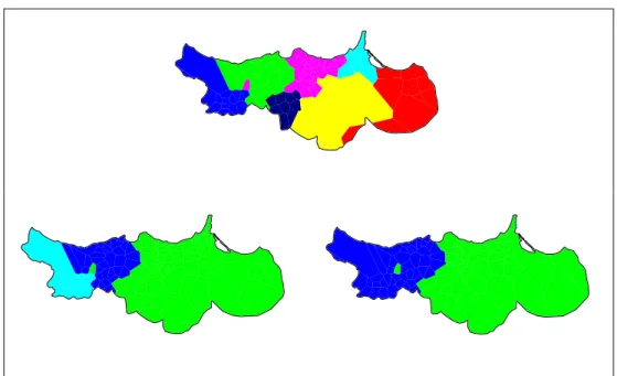
The lexis classification obtained through Lv distance corresponds with an asymmetrical configuration of 7 clusters which are structured into 2 major clusters distanced from one another by 8.08 (Figure 4). The matching dendrogram shares the same linguistic main delimitation (between groups 6 and 3-4) with the other dendrograms. This observation is corroborated by the CALv maps displayed in Figure 5, of which the 2-cluster map clearly indicates the most distinctive linguistic boundary. It is important to note that the CALv map (Figure 4) shows a distribution of the varieties similar to the CABin distribution, even though the composition of their respective dendrogram is divergent. 1 2 3 4 5 4 5 3 1 2 3
Figure 4: Dendrogram vs. CA Map - Lv – All lexis
’Arwi Bni WkilAfsu Tizdudin Iqedduren Saka
Gersif Hasi Berkan ’Ayn Zura-Ayt Heqqun Ayt Hidra Wlad Melluk Driwc Mezgitam-Ayt Hmed Hbircat Ayt Dawed
Ifettuchen Ayt Muhend U ’Abdellah
Ayt Waklan Tafughalt Thgasrut Tawrirt Zegzel Bni Buzeggu Berkan Zayyu
Cabo de Agua-Imrabden/Ayt Yusef Qaryat Arkman-Mellah
Acnur- Tighezdratin Ayt Hmu ’MarSuyyah I’etmanen-Rbardun Ajdir-Tara Tazeghwaxt Bured
Ayt Mhend Ayt Hazem Tizi Wesri - Ayt Ziyyan
Amejjaw Dar Kebdani Tazaghin
Isarhiwen Iyar n Tzaxt
Meqdada Sidi Hsayn Amzzawru La’zib n Sidi C’ayb u Meftah Raba’ n Trugut Ayt Bu Ya’kubAyt Mayyit Ayt Marghnin-I’ewwaden Ayt Ta’ban Ayt Tayar-Sidi Dris
Ayt Ya’qub Bu’diyya Ifasiyen Budinar Ayt Buhidus Ayt YarurBuhfura Yarzuqen Hammuda Ben Teyyeb
Mhajar Tariwin
Tawarda Ayt ’Azza Igarduhen Iyarmawas-Friha Tlata Uzlaf Talamghacht Tawrirt n wuccen Iyarmawas-Ijarayen
La’zib n Midar Midar Alto-Icennuden
Raq Azirar Aghir Umedgha At Buyefrur-Zghenghen Imezzujen-Ayt Nadur-Ice’aren Selwan Imezzujen-Ifarxanen-I’emranen
Ayt Nsar Ayt Sidar-Rabe’ n Trat
Bumiyya Burtwal Tifasur XadebCabo de Tres Forcas-Qabddenya Had n Ayt SicarIcemraren Ibuyqeddiden Ihninaten Imehhuten
Imezzujen-Ifarxanen-Ijuhraten Tibuda I’zanen-Sidi Lehsen Aduz Bades Tawssart Taghza Tara Yusef Bughembew Izemmuren Maya Tafnessa Ayt ’Abdellah-Icibanen Ayt Bu’iyyach Tmasint-Zawiyet n Sidi ’Isa Mulay ’Abd Qader
Timerzga-Tafsast Ayt Hicem-Idij
Ayt Qamra-Rwaz Imzuren Mnud-Ayt Hicem Ayt Hdifa-Tazrut Azru n tili Tizi Bni Budjay Aghir Hmed
Asammar Wad Mahkim
Ayt Hmed Sidi Bucetta Tazrut Ufis L’ars Tufist-ImurutenIgzennayen Bu’di Iharunen A’raben Azila Tamadda Luta Mazuz Lqel’a Ssaqya Tarya Aghennuy Wersan Tizirt Asammer Lmexzen Ssahel 0 2 4 6 8
Figure 5: CALv maps – 7 clusters vs. 3 clusters vs. 2 clusters – All lexis
1 2 3 4 5 6 7 7 6 4 3 1 5 2 4
2.5.2. Visualisation and interpretation of the MDS analyses
The MDS technique has the major advantage of ensuring objectivity and accuracy during the analysis stage of the materials because it excludes any external parametering. For example, the number of clusters cannot be changed because the analysis system provides it automatically. Each variety has its own colour. The colour contrasts are used to interpret the compared linguistic data: a colour continuity points to a perfect correlation between lexemes, while a colour mosaic reveals a low correlation between them.
The Rif region is divided into 7 major areas, regardless of the distance measuring applied (Figure 6). The distribution of the varieties on the MDS maps is almost similar to Bin and GIW; only a few minor differences in shades of certain colours were observed. The MDSLv map closely resembles the other two; the only significant distinction observed is the emergence of a small subdivision inside the group of Western varieties.
3. Contrastive results
Because of its accuracy, the MDS method is most appropriate for dialectometry analysis of Berber lexis. Accordingly, it forms a yardstick against which other dialectometry methods can be contrasted. Among the Cluster Analyses classifications (CA), CABin and CALv join best the distribution maps displayed by MDS (7 groups). Moreover, the CALv classification shows a further refinement because it takes into account the phonic variation of the units as much as their arrangement in the lexemes. However, any analysis based on Lv distance (CA as well as MDS) ignores the existence of the hierarchy between the phonic units (phonetic units= phonemic units), unless various weights are granted to them through a specific parametring. This method implies the construction of a phonological system within the software, involving a time and energy-consuming effort that is much too expensive compared to its profits.
Figure 7: CALv vs. MDSLv vs. CACLv maps
CALv
The Cluster Analysis classification has the benefit of precisely indicating significant linguistic boundaries. The CAC maps (Composite Cluster map; Figures 7 and 8) designate these boundaries by dark lines. Compared to the distinctive boundaries drawn by the dendrograms and CA maps of Figures 2 to 5, the principal linguistic delimitation of the CAC map of Figure 7 is drawn further to the West. It is important, nevertheless, to note that the CAC maps do not seem suitable to display the classification of Rif-Berber lexis because of the difficulty of interpreting the data, due to their rather chaotic representation (Figure 8).8
Figure 8: CAC – Bin vs. GIW vs. Lv maps – All lexis
Bin
References
Chambers J. K. & Trudgill, P. 1998. Dialectology. Cambridge, Cambridge University Press, 2nd edition.
Daan, J. & Blok, D. P. 1969. Van Randstad tot Landrand; toelichting bij de
kaart: Dialecten en Naamkunde, volume XXXVII of Bijdragen en
mededelingen der Dialectencommissie van de Koninklijke Nederlandse Akademie van Wetenschappen te Amsterdam. Amsterdam, Noord-Hollandsche Uitgevers Maatschappij.
Forquet, J. 1956. Linguistique structurale et dialectologie, Festgabe Frings, 190-203.
Garde, P. 1961. Réflexions sur les différences phonétiques entre les langues slaves, Word, XVII : 34-62.
Goebl, H. 1982. Dialektometrie; Prinzipien und Methoden des Einsatzes der
numerischen Taxonomie im Bereich der Dialektgeographie,
Philosophisch-Historische Klasse Denkschriften, volume 157, Vienna, Verlag der Osterreichischen Akademie der Wissenschaften.
Goebl, H. (1993). Probleme und Methoden der Dialektometrie: Geolinguistik in globaler Perspektive. In: Viereck, W. (ed.), Proceedings of the
International Congress of Dialectologists, Stuttgart, Franz Steiner Verlag,
volume 1, 37–81
Goossens, J. 1965. Die niederländische Strukturgeographie und die “Reeks
Nederlandse Dialectatlassen”, Bijdragen en mededelingen der Dialectencommissie van de Koninklijke Nederlandse Akademie van Wetenschappen te Amsterdam, volume XXIX , Amsterdam, N.V. Noord-Hollandsche Uitgevers Maatschappij.
Goossens, J. 1969. Strukturelle Sprachgeographie. Eine Einführung in
Methodik und Ergebnisse. – Heidelberg.
Grosse, R. 1960. Strukturalismus und Dialektgeographie. – Biuletyn
Fonograficzny, III : 89-101.
Heeringa, W. 2004. Measuring Dialect Pronunciation Differences using
Levenshtein Distance. PhD. Dissertation, Groningen, Rijksuniverstiteit
Groningen.
Hoppenbrouwers, C. & Hoppenbrouwers, G. 1988. De feature frequentie-methode en de classificatie van Nederlandse dialecten. – TABU, Bulletin
voor taalwetenschap, 18(2) : 51-92.
Hoppenbrouwers, C. & Hoppenbrouwers, G., 2001. De indeling van de
geklasseerd volgens de FFM (feature frequentie methode). Assen,
Koninklijke Van Gorcum.
Kessler, B. 1995. Computational dialectology in Irish Gaelic. In:
Proceedings of the 7th Conference of the European Chapter of the Association for Computational Linguistics, Dublin, EACL, 60–67.
Kruskal, J. 1999. An overview of sequence comparison. – In : D. Sankoff & J. Kruskal (eds.), Time Warps, String Edits, and Macromolecules: The
Theory and Practice of Sequence Comparison, MA, Addison-Wesley,
1-44.
Lafkioui, M. 2007. Atlas linguistique des variétés berbères du Rif, Köln, Rüdiger Köppe Verlag (in Berber Studies, volume 16), 2007, 291 p. (format « A3 », in color, 356 maps + 47 tables).
Lafkioui, M. forthcoming 1. Etudes de géographie linguistique berbère : variation géolinguistique et classification dialectométrique, Le Bulletin
des Séances de l’Académie des Sciences d’Outre-Mer, 22 p.
Lafkioui, M. forthcoming 2. Pour la recherche dialinguistique du berbère. Le cas du tarifit. In: A. El Aissati (ed.), From Oral Discourse Analysis in
Berber to Academic Language Skills in Dutch, Harrossowitz, 9 p.
Lafkioui, M. forthcoming 3. Analyses dialectométriques du lexique berbère du Rif, Studien zur Berberologie/Etudes Berbères, 4, 19 p.
Martinet, A. 1972. Structural dialectology, Pakha Sanjam, N° Spécial.
Moulton, W. G. 1960. The short vowel systems of northern Switzerland.
Word, 16 : 155–182.
Nerbonne, J. & Heeringa, W. 1998. Computationale vergelijking en classificatie van dialecten. – Taal en Tongval, 50(2) : 164-193.
Nerbonne, J. & Heeringa, W. 2001. Computational Comparison and Classification of Dialects. – Dialectologia et Geolinguistica, 9 : 69-83. Rensink, W. G. 1955. Dialectindeling naar opgaven van medewerkers.
Mededelingen der Centrale Commissie voor Onderzoek van het NederlandseVolkseigen, 7: 20–23.
Weijnen, A. (1946). De grenzen tussen de oost-noord-Brabantse dialecten onderling. In: Oost-Noordbrabantsche dialectproblemen: lezingen
gehouden voor de dialectencommissie der Koninklijke Nederlandsche Akademie van Wetenschappen op 12 april 1944, Bijdragen en
meededelingen der Dialectencommissie van de Koninklijke Nederlandse Akademie van Wetenschappen te Amsterdam, Amsterdam, Noord-Hollandsche Uitgevers Maatschappij, volume VIII, 1-15.
Weijnen, A. (1966). Nederlandse dialectkunde. Studia Theodisca. Assen, Van Gorcum.
Weinreich, U. 1954. Is a structural dialectology possible?, Word, 10 : 388-400.
Winkler, J. 1874. Algemeen Nederduitsch en Friesch Dialecticon. ’s-Gravenhage, Martinus Nijhoff.