HAL Id: hal-01971920
https://hal.archives-ouvertes.fr/hal-01971920
Submitted on 24 Jan 2021
HAL is a multi-disciplinary open access
archive for the deposit and dissemination of
sci-entific research documents, whether they are
pub-lished or not. The documents may come from
teaching and research institutions in France or
abroad, or from public or private research centers.
L’archive ouverte pluridisciplinaire HAL, est
destinée au dépôt et à la diffusion de documents
scientifiques de niveau recherche, publiés ou non,
émanant des établissements d’enseignement et de
recherche français ou étrangers, des laboratoires
publics ou privés.
Effective radiative properties of bounded cascade
nonabsorbing clouds: Definition of the equivalent
homogeneous cloud approximation
Frédéric Szczap, Harumi Isaka, Marcel Saute, Bernard Guillemet, Andrey
Ioltukhovski
To cite this version:
Frédéric Szczap, Harumi Isaka, Marcel Saute, Bernard Guillemet, Andrey Ioltukhovski. Effective
ra-diative properties of bounded cascade nonabsorbing clouds: Definition of the equivalent homogeneous
cloud approximation. Journal of Geophysical Research: Atmospheres, American Geophysical Union,
2000, 105 (D16), pp.20617-20633. �10.1029/2000JD900146�. �hal-01971920�
JOURNAL OF GEOPHYSICAL RESEARCH, VOL. 105, NO. D16, PAGES 20,617-20,633, AUGUST 27, 2000
Effective radiative properties of bounded cascade
nonabsorbing clouds' Definition of the equivalent
homogeneous cloud approximation
Fr6d6ric
Szczap,
Harumi Isaka, Marcel Saute, and Bernard Gulllerner
Laboratoire de M6t6orologie Physique, Universit6 Blaise Pascal, Aubii•re, France
Andrey Ioltukhovski
Keldish Institute of Applied Mathematics, Moscow
Abstract. In the present
study
we investigated
the r•di•tive properties
of inho-
mogeneous
nonabsorbing
clouds
under
the Equivalent
plane-parallel
Homogeneous
Cloud
Approximation
(EHCA),
by using
the one-dimensional
(l-D) bounded
cascade
inhomogeneous
clouds. The effective
optical depth was defined
under the EHCA
by requiring
the identity
of the radiant
flux components
of the radiation
budget
between
the inhomogeneous
clouds
and their equivalent
homogeneous
counterparts.
Such
requirement
provides
a rational
framework
to define
the effective
optical
depth
of the inhomogeneous
nonabsorbing
clouds.
We analyzed
the dependency
of the
effective
optical
depth
on the horizontal
scale
of averaging
and
solar
incidence
angle
and specified
the conditions
under
which
an inhomogeneous
cloud
segment
could
be
treated as a plane-parallel
homogeneous
cloud. A parameterization
of the effective
optical
depth was proposed
as a function
of the mean
optical
depth and a relative
cloud inhomogeneity
parameter.
Finally, we compared
the EHCA with the effective
thickness
approximation,
both based
on the definition
of the effective
optical
depth,
and discussed
the difference
between
their respect,
ive effective
optical
depths.
1. Introduction
Clouds exhibit fluctuations of microphysical charac- teristics at different spatial scales. How this spatial
inhomogeneity of cloud properties affects the radiative
transfer is one of the major issues of the atmospheric radiation theory. Many physicists have recently inves- tigated the problem of cloud inhomogeneity with re-
newed interest. Some have attempted to evaluate its effect on radiant flux components of the cloud radiation
budget
[Barker, 1992, 1996a,
b; Barker et al., 1996; Ca-
halan et al., 1994a; Marshak et al., 1995b, 1998; Borde and isaka, 1996; Chambers et al., 1997; Oreopoulos and
Davies,
1998a,
b; Oreopoulos
and Barker, 1999]. Others
have analyzed the statistical characteristics of the radi-ation fields
of natural clouds
by using
Landsat
and/or
AVHRR images [Barker and Davies, 1992; Davis et al., 1997: Marshak et al., 1995], or in situ measuren•en•s
[ Cahalan
and Snider,
1989;
Davis
et al., 1996,
1999].
In
these studies the emphasis was put on the interaction of the radiative transfer process with the "sub-cloud scale"fluctuations of microphysical properties as well as on
Copyright 2000 by the American Geophysical Union.
Paper number 2000JD900146.
0148-0227 / 00 / 2000JD 900146509.00
its scaling and auto-similarity properties. The spatial
scales
of the cloud inhomogeneity
co•sidered
i• these,
studies differ significantly from those considered it• the earlier studies on the broken cloud fields. in which the radiative interaction was considered between isolatedclouds
with simple
geometrical
shapes
[McKee
and Co:c,
1974;
Aida, 1977;
Davies,
1978;
Schmetz,
1984;
Brdon,
1992;
Barker,
1994;
Zuev and Titov, 1995].
Another
issue
emphasized
in these
studies
is the easy
and fast,
calculation
of the radiant flux components
of
the radiation
budget
of the inhomogeneous
clouds
in
general circulations models (GCMs). We can distin- guish schematically two approaches to this calculation:
the independent
pixel approximation
(IPA) proposed
by Cabalan
et al. [1994b]
and its variants,
and the Ef-
fective
Thickness
Approximation
(ETA) also
proposed
by Cahalan
et al. [1994a]
and its variants. These
two
approaches are sometimes confused and considered asequivalent.
However,
there is a significant
conceptual
difference
between
the ETA and the IPA, although
the
ETA was
initially
introduced
through
the area
averag-
ing of the IPA radiant
fluxes. It is revealing
that the
gamma
IPA [Barker,
1996b],
mentioned
below,
did not
invoke
an effective
optical
depth, which
suggests
that
the concept
of effective
optical depth and effective
ra-
diative properties, in general, is not an inherent element of the IPA.
20,618 SZCZAP ET AL.: RADIATIVE TRANSFER IN INHOMOGENEOUS NONABSORBANT CLOUDS
Cabalan et al. [1994b] showed that the IPA could
provide an "accurate" area-averaged reflectance of the bounded cascade inhomogeneous clouds at mesoscale.
Its extension to the cloud pixels or cloud segments was done as the nonlocal independent pixel approximation
(NIPA) by Marshak et al. [1995b, 1998] and as the gamma IPA by Barker [1996b] and Barker et al. [1996].
The applicability of the gamma IPA depends on that of the IPA. since it is proposed as a computer-efficient ap-
proximation to the IPA [Barker, 1996]. The IPA and
its variants rely on the "error-smoothing" effect of area averaging to calculate the area-averaged radiant fluxes of the inhomogeneous clouds. Accordingly, the IPA is not necessarily restricted to the bounded cascade type of inhomogeneous clouds. Furthermore, since the av- eraging is a simple linear operation, the IPA assumes implicitly that the interaction of the radiative transfer process with the cloud inhomogeneity does not exhibit a large nonlinear effect when the radiant fluxes are av- eraged over an area large enough to neglect [lie contri-
bution of the net horizontal photon transport,.
On the other hand, the ETA and its variants (the equivalent homogeneous cloud approxirnati(m we pro- posed below can be considered as one of them) aimed to treat the inhomogeneous clouds under t•he plane- parallel homogeneous (PPH) cloud assumption. The effective radiative parameters are defined by requiring
the identity of radiant flux components be[ween the in-
homogeneous cloud and their equivalent homogeneous
counterparts. The key element of this approach is the functional relations between the effective radiative pa- rameters and the mean radiative and structural param-
eters of the inhomogeneous clouds. Consequently, the
ETA and its variants are not to be considered only as
a method of radiant flux calculation as the IPA but
a method to analyze the nonlinear effect of the "radia-
tive transfer-cloud inhomogeneity" interaction. which is
embodied by the above fimctional relations themselves.
When the ETA is used to calculate the radiant flux
components, the performance of the ETA should dif-
fer from that of the IPA according to the importance of the nonlinear effect in the "radiative transfer-cloud
inhomogeneity" interaction.
A fractal or multifractal cloud could be treated un-
der the PPH cloud assumption and its effective opti- cal depth be expressed as a function of the cloud in-
homogeneity [Cahalan et al., 1994b: Borde and Isaka,
1996]. However, in these studies the cloud inhomogene-
ity was represented by fractal parameters of the cascade
processes used for the inhomogeneous-cloud generation. Therefore their effective optical depths are applicable
only to the scale of the entire cloud domain but not to
the scale of a cloud segment. Furthermore, such frac-
tal parameters are only relevant to the inhomogeneous
clouds generated with those specific cascade processes (bounded cascade in the work of Cahalan et al. and lognormal cascade in the work of Borde and Isaka) but not to the clouds generated with other cloud-generation
processes. Hence there is a need to investigate how the ETA approach can be extended to the cloud segments, but also to define pertinent parameters to represent the nonlinear effect of the cloud inhomogeneity at the scale
of cloud segments.
In most of the above studies, the emphasis was put
only on the reflectance or albedo of the inhomogeneous clouds and its approximation. However, for GCM ap- plications we need to consider not only the energy re-
flected from the clouds but also the other radiant flux
components (absorptance and transmittance) of the ra-
diation budget. For example, we have to compute, in some case, the radiation budget of inhomogeneous clouds with highly reflecting underlying earth surface.
Doing so under the plane-parallel homogeneous cloud
assumption requires the precise definition of an equiv- alent plane-parallel homogeneous cloud and its effec- tive radiative properties within an adequate theoretical framework. From this point of view, the EHCA can be considered as an attempt to develop the ETA approach within a more fbrmal framework and then to extend it to the inhomogeneous absorbing clouds [$zczap et al., this issue].
The retrieval of cloud parameters from remotely sens-
ed multispectral radiometric data is another field of in-
terest in which we have to consider the cloud inhomo-
geneity. The actual cloud parameter retrieval assumes that a plane-parallel homogeneous cloud model is valid
at the scale of one satellite image pixel [Nakajima and
King, 1988, 1990; Twomey and Cocks, 1989; Wetzel
and Vondcv Haar, 1991]. This implies that when the
optical depth is retrieved, it is effective and not av- erage optical depth. To correct the effect of the sub- pixel scale cloud inhomogeneity on the retrieved optical depth requires the knowledge of the functional relation
between the effective optical depth and the mean rameters (mean optical depth, subpixel scale cloud in-
homogeneity). This would be within the scope of the
ETA arid its variants (T. Faure et al.. Nem'al network
retrieval of ('loud parameters of inhomogeneous and
fi'actional clouds from multispectral reflectance data:
feasibility study. submitted to Remote Sensing of En- vironment, 1999c (hereinafter referred to as F99c)) but not within the scope of the IPA and its variants. For
example, Marshak et al. [1995b] attempted to retrieve
the optical depth of inhomogeneous clouds directly from high-resolution radiometric data under the NIPA. How- ever, this approach as such is not applicable to mod- erate resolution radiometric data (advanced very high resolution radiometer (AVHRR), Moderate-Resolusion Imaging Spectroradiometer (MODIS), global imager on adeos 2) (GLI), because it cannot take into account the subpixel scale cloud inhomogeneity. This problem in it- self differs from the one investigated at multipixels scale
by Barker et al. [1996] and Davis et al. [1997].
The purposes of this study are to answer the differ- ent questions asked above: (1) to define the effective optical depth under the equivalent homogeneous plane-
SZCZAP ET AL.: RADIATIVE TRANSFER IN INHOMOGENEOUS NONABSORBANT CLOUDS 20,619 parallel cloud approximation (EHCA) with the require-
ment of identity of the radiant flux components between the inhomogeneous clouds and their homogeneous coun- terparis; (2) to specify the conditions under which an inhomogeneous cloud segment can be treated under the plane-parallel homogeneous cloud assumption; (3) to analyze the dependency of the effective optical depth on the horizontal averaging scale and solar incidence angle;
and (4) to derive an empirical equation relating the ef-
fective optical depth to the local mean optical depth and a relative cloud inhomogeneity parameter. Finally, we
discuss the basic difference between the EHCA and the
ETA [Cahalan
et al., 1994a,
b]. This study is based
on
the use of (I-D) bounded cascade inhomogeneous cloud as in most of the studies mentioned above, excluding
the broken cloud fields from our scope. X•5 - discussed,
elsewhere, the extension of the EHCA to the inhomo-
geneous absorbing clouds [$zczap et al., this issue I and 2-D inhomogeneous clouds [Szczap et al., 20001. The ap-
plication of the EHCA to [he cloud parameter retrieval
is discussed by F99c.
2. Conditions of Simulation
2.1. Monte Carlo Radiative Transfer Code The Monte Carlo (MC) method is the simplest nu-
merical tool to compute the radiative transfer' in an
arbitrarily inhomogeneous rnedium. Assuming the ex-
tinction coe•cient and single-scattering albedo inde-
pendent of the incident direction, we can write the ra- diative transfbr equation
7(fi,
where
I(•, •) designates
the
radiant
intensity
along
a
direction
vector at a point 7, a(½) and •(½) are the
extinction coe•cient and the single-scattering albedo atpoint
½; 7(•, t?) is the volume
scattering
phase
fimc-
tion from an incident direction •' to another direction
•. The replacement of • with a? yields
7(fi, ff')ff',
(2)
where • is a similarity coe•cien[. Because of this iden-
tity of radiation fields for homo[hetic media, we can
use a fixed cloud domain for our simulation of radia-
tive transfer in inhomogeneous clouds without, much loss of generaliW. In the maximal cross-section method
[Marchuk
et al., 1980; Marshak
et al., 1995a],
equa-
tion (1) is transformed into+
• Gmax
O'??l a x
- --)6(5
-
ff,)aff,,
(3)
where a•x represents the maximum extinction coeffi-
cient in the cloud domain. We used the MC code [Mar- shaket al., 1995a] for both the homogeneous and the
inhomogeneous clouds.
2.2. Generation of Bounded Cascade
Inhomogeneous Clouds
For MC simulation we have to generate inhomoge-
neous clouds with prescribed characteristics of cloud inhomogeneity. Fractal and multifractal analyses were recently used to study the scaling and autosimilarity
properties of natural clouds and cloud fields [Lovejoy,
1982; Cabalan, 1989; Duroure and Gulllerner, 1990; Ca-
halan et al., 1994a; Marshak et al., 1995b], but also to simulate synthetic inhomogeneous clouds [Scherzter a•d Lovejoy, 1991; Davis et al., 1994]. A multifrac-
tal medium can be generated with the lognormal cas-
cade process tMonin and Yaglom, 1975], but it tends to
produce "unrealistic" intermittent fluctuations of cloud
properties. Cabalan et al. [1994a] and Mayshah et al. [1994] proposed a bounded cascade process in which the
L
m•lltiplicat, ive factor IV,• varies with the scale r,• = 2,•
at step n like
1- 2p
n:. - 1 + 2(r•-l)H ' (4) where the plus and minus signs occur with equal prob-
ability, and H and 2p are usual fractal parameters of
the bounded cascade process [Marshak, 1994]. The bounded cascade model remedies the -1 limitation of the spectral slope that constitutes a major flaw of the
lognormal process. Furthermore, the bounded cascade
inhomogeneous clouds are considered as a fair approx- imation to 1-D horizontal fluctuations of liquid water
path within low-level stratiform clouds [Cah, alan et al.,
1994a].
The model parameters H and 2p were set equal to 0.25 and 0.50; then, the power spectrum of the opti-
cal depth fluctuations has a theoretical spectral slope of -1.5. The cloud domain is of 12.8 km in the hor-
izontal and 0.3 km in the vertical. It is composed of 256 elementary "bar" cloud pixels, each one of which is 50 m wide in the x direction and infinite in the y
direction. The number of cascades and the horizontal extent of cloud domain are chosen in such a way that the inhomogeneous clouds be characterized by a mod-
erate to large standard deviation of fluctuations in the
optical depth when averaged over a scale of kilometers. The cloud domain is repeated horizontally to obtain an
inhomogeneous cloud of infinite horizontal extent. The optical depth, hence the liquid water content, is assumed to be vertically uniform in each cloud pixel; the
fluctuations of the optical depth correspond to the fluc-
tuations of the droplet concentration. The droplet size
distribution is of the C1 type, and the volume-scattering phase function is computed for monochromatic light of
0.55 /zm [Garcia and Sicweft, 1985]. The asymmetry factor (g = 0.848 at 0.55 /tin) does not change signifi-
20,620 SZCZAP ET AL.' RADIATIVE TRANSFER IN INHOMOGENEOUS NONABSORBANT CLOUDS
cantly for droplet size distributions usually observed in
low-level stratiform clouds [Davies et al., 1984]. On the other hand, Borde and Isaka [1996] showed that its ef-
fect on the effective optical depth is linear, and it should
remain small in our case.
We generated independently an inhomogeneous cloud for each M C simulation. For a given solar zenithal angle
6}o, M C simulation was carried out for different values of
the mean-cloud optical depth • (from 1 to 60); we some- times qualify a mean optical depth as "cloud- mean" to stress that the mean is taken over the entire cloud do- main (12.8 km) and not over a cloud segment. For each
•, we generated three independent clouds by varying the seed of the cascade process and realized MC simulation
for each one of them. The exception to this is a series of special simulations discussed in the subsection 3.1.3.
MC simulations were done, by using 3 x l07 photons (approximately 1.2 x 10⁵ photons/cloud pixel). We
computed the reflectance and transmittance for each cloud pixel and the area-averaged reflectance and trans- mittance over cloud segments of L. The MC method has
an intrinsic statistical error, which decreases with the
increasing number of photons. When the average re- flectance and transmittance were computed over a seg-
ment 0.8 km wide, the relative error remains less than
about 5 x l0 -3 (Appendix A). Since L = 0.8 km is
the smallest scale of averaging in this study, this value constitutes the upper bound of the relative error in thereflectance and transmittance reported below.
3. Analysis of Monte Carlo Simulations
The plan of the present analysis is as follows. In subsection 3.1, we study how the horizontal averagingscale affects the effective optical depth of inhomoge-
neous clouds and discuss the conditions under which the plane-parallel homogeneous (PPH) cloud model can be applied to the bounded cascade inhomogeneous clouds.
In subsection 3.2, we establish a relation between the
effective optical depth, the mean optical depth, and cloud inhomogeneity parameter. Finally, the differ- ence between the EHCA and ETA is discussed in sub- section 3.3. When an inhomogeneous cloud is gener- ated with a cascade process, the first few steps of the cascade condition the fluctuations at large horizontal scale. Accordingly, these fluctuations cannot be con- sidered "completely random" because of a very limited
number of possible configurations [Monin and ¾aglom, 1975]. Hence, we randomized the cloud segment loca- tions within the entire cloud domain to eliminate even- tual systematic bias that could result from this limited configuration number.
3.1. Equivalent Homogeneous Cloud, Effective Optical Depth and Horizontal Averaging Scale
3.1.1. Equivalent homogeneous cloud approx-
imation. Let us define a PPH cloud equivalent to an
arbitrary inhomogeneous cloud by requiring that it has
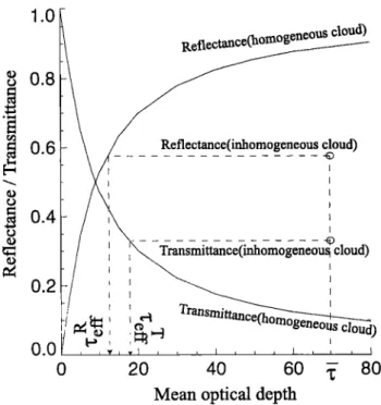
1.0 0.8
0.6
0.4 0.2 0.0 0Reflectance(homogeneous
cloud)
Reflectance(inhomogeneous cloud) i Transmittance(inhomogeneou• cloud)'"' •
•"]
,
40
60 y
80
Mean optical depth
Figure 1. Schematic representation of the method used
to determine
•-•%
and •-e• of an inhomogeneous
cloud
segment from its "measured" reflectance and transmit-
tance.
either the same reflectance or transmittance as that of
the inhomogeneous cloud. The reflectance and trans- mittance of a P PH cloud are shown in Figure 1 as a function of the optical depth for a given solar incidence
angle. The effective optical depth can be defined from
either
the
reflectance
r•%
or transmittance
r•[ according
to the following relations:
/•hom
(T•/•,
6}o)
-- /•inhom
(•, 6}0)
Tho
m (Tfff,
6}0)
-- Tinhorn
(•, 6}0),
or
(5)
'- /i•ho
m [/r•inhom
(f, 6}0),
6}0]
T --1
•'•ff -- Tho
m [Tinho
m (•, 6}0),
6}o],
or
(6)
where f designates the cloud-mean optical depth of an inhomogeneous cloud, Rhom and Thom, respectively, the
reflectance and transmittance of its equivalent homoge- neous cloud.
The equivalent homogeneous cloud defined above does not have necessarily the "same reflectance and same transmittance" as that of the original inhomogeneous
cloud,
because
its r•%
and
r•[ do not necessarily
agree
with each other. The radiation budget of an inhomo-
geneous cloud or cloud segment can be treated under
the PPH cloud
assumption,
only
when
r•%
and
r•[ are
identical within a prescribed error. The requirement of
the identity between these two effective optical depths
is the essential element of the EHCA; the effective op-
tical depths defined in Cahalan et al. [1994b] or Borde and Isaka [1996] are not based on such requirement. In
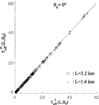
SZCZAP ET AL.' RADIATIVE TRANSFER IN INHOMOGENEOUS NONABSORBANT CLOUDS 20,621 60[-
t
o:O
ø
/ / /4o
2O O ' L-•.2 km + ß L-1.6 km 0 2O 40 6OT (L,00)
Figure 2. Comparison
between
•-• and •-• obtained
from the reflectance and transmittance of inhomoge-
neous cloud segments. Horizontal averaging scale: œ-
3.2 km and œ - 1.6 km; solar' incidence angle 00 - 0 ø
the horizontal scale of averaging on the effective optical depth, by considering inhomogeneous cloud segments
wit, h a horizontal extent L. Then, we will refer to the
eff(-('tive optical det)th of such cloud segments as •qocal effective optical depth" :-eft(L).
3.1.2. Dependency of *'eft(L) on the horizon-
[al averaging scale In Figure 2, we plotted •_R
' eft(L)
60
80
= 300
0 20 4o 6o
'lj r (L,00)
eftFigure 3. Same as Figure 2 but for 00 - 30 ø
against
re•f(L
) for the vertical
incidence
and for two
scales
of averaging
(3.2 km and 1.6 km). Value
re•(L
)
differs
little from
the corresponding
r•(L) for both
the
scales of averaging. This suggests that when vertically illuminated, an inhomogeneous cloud or cloud segment of these horizontal scales can be treated as a P PH cloud if the effective optical depth is used instead of the cloud-
mean optical depth. Figure 3, which is the same as
Figure 2 but for a solar zenithal angle 30 ø, exhibits the same general feature of variations except that the dis- persion around the bisector is larger in Figure 3 than in Figure 2. The larger dispersion is partly due to an
increase in the net horizontal photon transport between
the cloud segment and its neighboring cloud pixels with the increasing solar incidence angle.
We defined the relative dispersion as
Ddisp
-- V/sin
2
ct
(7)
where N is the total number of data. The relative dis-
persion represents the root-mean-square of sin a, where
a is the angle between
the vector rr R r •
• eft' eft/and the
bisector;
we use (r;•r, rfff)instead
of [re•(L), r•(L)]
when there is no risk of confusion. Since we were inter-
ested in the difference between rT and •
eft
r•ft.
, we preferred
to estimate this relative dispersion instead of using the
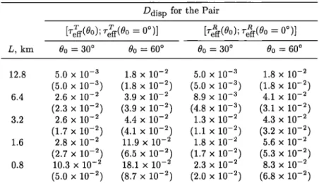
usual linear' regression analysis. Another reason fox' this choice is that the relative dispersion can be easily re- lated to the net horizontal photon transport as shown in section 3.1.4. Table 1 represents the relative dis-
persions for three incidence angles and five horizontal scales of averaging. We also computed the second esti- mates of the relative dispersion by using only the data with reft > 1.• , because the relative error tends to
Table 1
ßRelative Dispersion
Between
r T and •
eft eftAround the Bisector as a Function of the Scale of Av-
eraging
Ddisp
Between
refT
t and ref tL, km Oo - 0 ø Oo - 30 ø Oo = 60 ø 12.8 7.7 x 10 -5 6.7 x 10 -5 2.2 x 10 -5 (9.7 x 10 -6 ) (1.1 x 10 -s) (1.2 x 10 -s) 6.4 1.3 x 10 -2 1.8 x 10 -2 5.2 X 10 -2 (8.1 x 10 -s) (1.9 x 10 -2 ) (5.4 x 10 -2 ) 3.2 1.8 x 10 -2 5.7 x 10 -2 7.7 x 10 -2 (9.6 x 10 -2) (3.4 x 10 -2) (8.4 x 10 -2) 1.6 4.7 x 10 -2 9.9 x 10 -2 14.0 x 10 -2 (2.7 x 10 -2) (4.5 x 10 -2) (13.9 x 10 -2) 0.8 8.6 x 10 -2 14.2 x 10 -2 18.6 x 10 -2 x 10 (8.2 x (18.4 x
Numbers in parentheses are the relative dispersions esti-
20,622 SZCZAP ET AL.: RADIATIVE TRANSFER IN INHOMOGENEOUS NONABSORBANT CLOUDS
be larger for small reft(L) than for moderate to large reft(L ) . These estimates are given in parentheses in Ta-
ble 1.
For the 12.8
km averaging,
•-•[ and •-•%
of an inho-
mogeneous cloud should be identical for a given solar incidence angle, because of the periodic lateral bound- ary conditions. For all the three incidence angles the relative dispersions are close enough to zero. Hence
we can
conclude
that re•f(L
) and
r•f(L) of an inhomo-
geneous cloud are identical at this scale of averaging. For the other scales of averaging the relative disper- sion varies significantly with the solar incidence angle;
it ranges from about 10 -2 for L = 6.4 km and 00 = 0 ø
to more than 10 -• for L = 1.6 km and 00 = 60 ø. When
the relative dispersion is computed only with the data
(reft > 1.5), it decreases
by about 50% (from 4.7 x 10
-2
and 9.9 x 10 -2 to 2.7 x 10 -2 and 4.5 x 10 -2 ) for 0 ø and
30 ø but remains practically unchanged for 60 ø (from
14.0 x 10 -2 to 13.9 x 10⁻²). Accordingly, when the
plane-parallel cloud assumption is applied to a given
horiz•)ntal
scale
of averaging,
its accuracy
is strongly
dependent on the solar incidence angle.The relative
dispersion
Ddisp
may be used
as a crite-
rion to define a minimal horizontal averaging scale be-
yond which the EHCA can be used without any serious error in the radiation budget of an inhomogeneous cloud
segment. We hereinafter abbreviate this "minimal scale
of averaging" as MSAv. From a practical point of view the determination of the MSAv depends on the errors of the radiant flux we can consider as "acceptable." If we
define
the MSAv
with the criterion
Ddisp
_• 5 x 10
-2, it
would be about 1.6 km for 0 ø, 3.2 km for 30 ø, and 6.4km for 60
ø respectively.
The value
of Ddisp
= 5 x 10
-2
in the effective optical depth corresponds to a relativeerror of 5% in the radiative fluxes in the range where
the radiative fluxes (reflectance and transmittance) vary
quasi-proportionally with the optical depth. For a large optical depth for which the radiative fluxes vary little
with
the optical
depth,
Ddisp
-- 5 x 10
-2 corresponds
to
a relative error much less than 5% for the reflectance,
while it corresponds to a relative error more than 5% for the transmittance. These MSAvs agree with the hor- izontal scales of averaging, estimated for the applica- bility of the plane-parallel cloud assumption by Barker
[1996].
•.1.•. Dependency of reff(L,0o) on the so-
lar incidence angle. According to the above results,
reef(L,
00)
and
r•f(L,
00)
of
an
inhomogeneous
cloud
es-
timated for a given 00 are almost identical when they are estimated for a sufficiently large scale of averag-
ing. However, this does not guarantee that reft(L , 00) is
independent of 0o , when reft(L, 00) of the same cloud
segment is estimated for different solar incidence angles. Table 2 lists the relative dispersions between reft(L, 00)
and reft(L, 0 ø) determined either from the reflectance or
the transmittance.
As expected,
Ddisp
increases
with
the decreasing scale of averaging and the increasing so- lar incidence angle. The dispersion is slightly smaller for•-• than for T.
r•f[, in other
words,
photons
going
through
eft
the entire cloud depth are more affected by the cloud in- homogeneity than those reflected from the upper part of clouds; in other words, the net horizontal photon transport does not affect the reflectance and transmit- tance in the same way. This may have an interesting implication to the cloud parameter retrieval from the up-welling radiation fields.
However, the relative dispersion is too global to an-
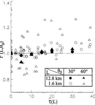
alyze in detail how reff(L,0o) varies with 00. Hence we computed the ratio r(L, 0o) = reff(L, Oo)/reff(L,0ø).
Figure
4 shows
r(L, 30
ø) and
r(L, 60
ø) of r• r estimated
Table 2. Relative Dispersion Between ref t for an Oblique Incidence
( 00 = 30 ø and 60 ø) and reft for the Vertical Incidence Ddisp for the Pair
- 0ø)]
= 0ø)]
L, km 0o = 30 ø 0o = 60 ø 0o = 30 ø 0o = 60 ø 12.8 5.0 x 10 -a 1.8 x 10 -2 5.0 x 10 -a 1.8 x 10 -2 (5.0 x 10 -a) (1.8 x 10 -2 ) (5.0 x 10 -a) (1.8 x 10 -2 ) 6.4 2.6 x 10 -2 3.9 x 10 -2 8.9 x 10 -a 4.1 x 10 -2 (2.3 x 10 -2) (3.9 x 10 -2) (4.8 x 10 -a) (a.1 x 10 -2) 3.2 2.6 x 10 -2 4.4 x 10 -2 1.3 x 10 -2 4.3 x 10 -2 (1.7 x 10 -2) (4.1 x 10 -2) (1.1 x 10 -2) (3.2 x 10 -2) 1.6 2.8 x 10 -2 11.9 x 10 -2 1.8 x 10 -2 5.6 x 10 -2 (2.7 x 10 -2) (6.5 x 10 -2) (1.7 x 10 -2) (5.3 x 10 -2) 0.8 10.3 x 10 -2 18.1 x 10 -2 2.3 x 10 -2 8.3 x 10 -2 (5.0 x 10 -2) (8.7 x 10 -2) (2.0 x 10 -2) (6.8 x 10 -2)Numbers in parentheses are the relative dispersions estimated for ref t _>
1.5. Effective optical depths are determined either from the reflectance
SZCZAP ET AL.' RADIATIVE TRANSFER IN INHOMOGENEOUS NONABSORBANT CLOUDS 20,623 i.4 1.2 0.8 0 • o
•
300 60
ø
12.8 km * ß 1.6 kxn o • ,_50 40Figure 4. Effect of •0 on r (L, •, ) =reft(L, •, )/reft(L, 0ø); •, = 30 ø and • = 60ø. Horizontal scale of averaging ß L = 12.8 km and
L= 1.6 km.
for two scales of averaging, 12.8 km and 1.6 krn, as a
f•nct, ion of' f(L). For the 12.8 km averaging, the ratios remain (;lose to 1 for both incidence angles. However,
a close examination reveals a slight systen•ati(' bias for both incidence angles' for example, r(12.8 kin, 60 ø) de- creases from 1 to about 0.93 as e increases f¾om 0 to
5, then increases to about 1.03 as e goes from ,5 to
40. For the 1.6 km averaging, r(1.6 kin, 30 ø) exhibits a
similar variation with e , and it goes up to about 1.08
for 20 _< e. Value r(1.6 kin, 60 ø) is much more scat-
tered; it varies between 0.8 and 1.2 for e < 10, while it
becomes mostly larger than 1 for 10 _< f. This find- ing implies that when an inhomogeneous cloud segment
with e < 10 is obliquely illuminated, it acts as a cloud
segment optically thinner than when it is vertically il- luminated, while for f >> 10, it acts as a cloud segment optically slightly thicker. Consequently, we cannot de- fine, strictly speaking, a unique equivalent homogeneous cloud for a given inhomogeneous cloud, because its ef-
fective optical depth would change with the solar inci- dence angle. However, if the averaging is taken over a
sufficiently large area, the solar-incidence-angle depen- dency of reft(L, 00) remains small and less than about 3% for most of the mean optical depth except around
We looked for the explanation of these systematic bi- ases. When a photon with an oblique incidence angle is transmitted through an inhomogeneous cloud layer, this photon follows a slant path through consecutive
cloud pixels having different optical depths. The local
slant optical depth encountered by this photon can be
computed from purely geometrical arguments and con-
verted into an equivalent vertical optical depth as shown in Appendix B. We determined the probability density
function (PDF) of this local equivalent vertical optical
depth for 00 -0 ø, 30 ø, and 60 ø
For the homogeneous clouds the P DF is given by a function, while for the bounded cascade inhomogeneous clouds, it is close to a lognormal PDF (Figure B1). As 00 increases, the PDF of the equivalent vertical optical depth exhibits a significant shift toward a larger op- tical depth and, at the same time, becomes narrower
and skewer to the benefit of large optical depths (Ta- ble B 1). These features represent the averaging effect of
the slant path through an inhomogeneous cloud; these
variations of the PDF with the incidence angle occur
without any change of the cloud-mean optical depth. They imply that an obliquely penetrating photon en- counters more frequently :'moderate to large" local op- tical depth than a vertically penetrating photon. This
may explain
why •-•ff(L) of an inhomogeneous
cloud
with a "moderate to large" mean optical del)Zh becomes larger for the oblique incidence than for tile vertical in- tiderice. Since tile contribution of multiple scattering
to the reflectance increases with the cloud-mean optical depth, the above effect would become more effective as the cloud-mean optical depth increases. However, this process cannot be used to explain the opposite effect;
that is, the decrease of r(L, 60 ø) observed for the mean
optical depth e < 10. To explain this decrease, we have
to ('onsider how the reflectance of the PPH and inhomo-
geneous clouds varies with e and 00, but also how the difference/•hom (e, 00) -/•,inhorn (•, t90 ) varies with these parameters. We will resume this discussion after the feet of tile net horizontal photon transport is analyzed
(equation (12)).
3.1.4. Effect of the net horizontal photon
transport on the effective optical depth. A vec-
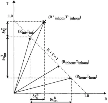
tor (/•hom, Thom) represents a PPH non-absorbing cloud
on the (/•, T) plane (Figure 5). For the condition of nil
net horizontal photon transport, the point (/•horn, Thorn)
moves on /• + T - 1 line, as the cloud optical depth varies. In this case, /• and T are dependent, and tile optical depth can be expressed as a function of either
the reflectance
r • - r(/•hom;00)
or the transmittance
r r - r(•hom; (•0). The reflectance
/•inhorn
and trans-
mittante Tinhorn of an inhomogeneous cloud with a given • differ from those of a homogeneous cloud with the same e. The displacement from (/•hom, Thorn) tO (/•inhorn,Tinhom) represents the effect of the cloud in-homogeneity.
If /•inhom
-1-Tinhorn
-- 1, both r•i7r
=
r(/•inhom;
Z,00) and r• - ';-(Tinhorn;
Z,00) still agree
with each other.
Let us consider the area-averaged reflectance and transmittance of an inhomogeneous cloud segment such
' Y' - 1 + e , where the quantity • in-
as /•inhorn d- inhom --
dicates an excess or deficit in the radiation budget of the segment due to the net horizontal photon trans- port into the cloud segment. The displacement from
20,624 SZCZAP ET AL.' RADIATIVE TRANSFER IN INHOMOGENEOUS NONABSORBANT CLOUDS
i
R
T 37-in[:
1 dr
l'01
(R
' inhom,T
' inhom)
• • [( inhom
--
Titnhorn)
--
(•hom
--
Thom)]-
(11)
• ....
[-'•,-
...
For
e
=
0,
equation
(9)
can
be
rewritten
as
•
(Ri• i
'"
:
- R
R -- • (•hom
dr
-- •inhom)' (12)
We can use equation (12) to analyze the feature,
•
••
r(12.8
kin,
60
ø)
< l for
e < 10,
observed
in
Figure
4.
•
•
The difference
(•hom- •nhom)0=0o
is always
positive
',, (Ri•om,Tinhom)
and goes
through
a maximum
at a certain
optical
depth
e•a•(00) as e increases. When the incidence angle
00 increases, e•,•(00) shifts toward a smaller e; this
'
(••••
Thom)
means
larger
than (Rhom-
that
for•<<
•maz
•nhom)0=0ø.
(00),
(Rhom
As for (dT/d•)o:0o,
- R•nhom)0=60
øis
(dr/dR)o=60o is larger than (dr/dR)o=0o as far as • is • larger than or not much smaller than •,,•(00). Ac-
' bx•R
d
R
"4
r bZin
t
1.0
Figure 5. Schematic diagram showing the positions of
a homogeneous
cloud
(R•om,
Tt•om
) and two inhomoge-
neous clouds with the same mean optical depth: the one
having
(/•inhom,
Tinhom)
and the other
(•inhorn'
Ti'nhom)
on the (R,T) plane. The first one has no net hor-izontal photon transport between the cloud segment
and adjacent cloud pixels Rinho m -1-Tinho m : 1 and
the second a finite net horizontal photon transport
' T.' - I + s, where the quantity • indi-
•inhom -1- inhom
--
cates an excess or deficit in the radiative fluxes.
into two displacement vectors, where (-/•hom ,Thom) are the reflectance and transmittance of a homoge-
neous cloud with the same f as the inhomogeneous
cloud. The first displacement is from (Rhom,Thom)
to a point (]•int,Tint) and the second from (]•int,Tint)
tO (•inhom
' inhom)
T'
.
The intersection
point (Rint,
•/•nt)
is determined
by drawing
the normal from (Rinho
m
, Titnhom)
OI1
• -• T - 1 line (see
Figure
15)'
_
i [1
-[-
(/r•inho
m
/•int •
'
inhom)]
_ i [1 -- (•inhom
-- Titnhom)]'
Tint
(8)
This decomposition enables us to express the relative
dispersion
as a simple
function
of •. For
re•(L
) we
have
67-e•
- 8right
+ 6'rfi
(9)
with
•Te• :
T(/•inhom;
L) - T(/r•hom)
•TiRnt
=
T(/r•int;
L) - T(/r•hom)
(10)
•Ts
R : 7-(•inho
m;
L) - 7-(•in
t; Z).
The first
term
5right
on the right-hand
side
represents
the
variation of the optical depth due to the displacement
along R + T- I line'
cordingly,
we may
have
[5%•(0- 0o)[ > 15%•(0- 0)l
with 5refit(0- 0o) < 0, if the increase
in (Rhom-
•inhom)0=0o overcompensates
the decrease in
(dr/dR)o=Oo
or the decrease
in (Rhom- Rinhom)O=Oo
is compensated by the increase in (dr/dR)o=Oo, and
this is what happens as shown in Figure 4. Con-
sequently, it is the way in which (dr/dR)o=Oo and
(•hom -- ]•inhom)0=0o
vary with the solar
zenith
angle,
and not the apparent increase in the slant path optical depth, that produces r(12.8 kin, 60 ø) < 1 for e < 10 observed on Figure 4. Consequently, the radiative pro- cesses that, produce r(12.8 kin, 60 ø) < 1 feature should be quite different from those contributing to the 1 <r(12.8 kin, 60 ø) feature.
As for the second term of equation (9), it represents the variation of the optical depth due to the excess or deficit in the radiation budget of the cloud segment. To estimate this term, we have to choose either reflectance
or transmittance:
-
•)_•
)
(13)The vector
(Sr•, 8•) represents
the displacement
from
the on-bisector point [r(Rint,00), r(Tint,0o)] to the off-
bisector
point
[7-(•inhom,
O0),7-(TitnhQjn
• •0)]. Consequen-
tly, there
is no identity
between
re(L ) and
as
far as the net horizontal photon transport between the cloud segment and the adjacent cloud pixels is not nil. The relative dispersion defined above can be expressed
as:
•7)disp
"'• •-• i:1
[
T7f•-•i'J2 (14)
with
where the index i indicates the ith data point and reft
is the effective optical depth. This equation shows that the dispersion depends directly on the s term.
SZCZAP ET AL' RADIATIVE TRANSFER IN INHOMOGENEOUS NONABSORBANT CLOUDS 20,625 Optical depth 00.1 05 1 2 5 8 10 15 •0 3040 80 oo 1.0
0.8
+
o.s
0.2[
0.0
•
... •
0,0 0.• 0.4 0.6 0.• •.0Reflectance
R'inho
m
Figure 6.
Reflectance
/•inhom
and transmittance
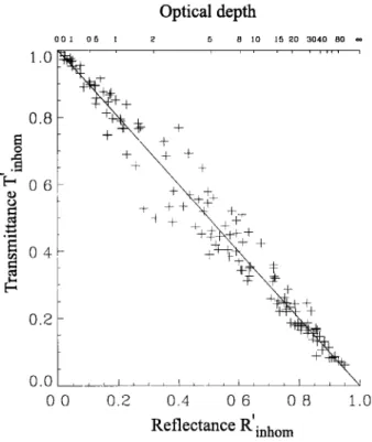
T.' inhom of the inhomogeneous cloud segments estimated for the 1.6 km averaging and for the 60 ø incidence.Figure 6 shows
all pairs (/•inhom,Titnhom)
obtained
for inhomogeneous cloud segments with L : 1.6 kmand 00 = 60 ø ß The dispersion around /•+T = 1, in
other words c term is larger for moderate reflectance
or transmittance
(1 < ½ < 10). As Titnhom
approaches
zero (large ½), tile penetration depth of photons be- comes small. Accordingly, the probability for these pho-tons to participate in the horizontal transport decreases
with the penetration depth [Marshak et al., 1998]. This
implies that the c term would become small as • in-
creases beyond a certain optical depth [Titov, 1998].
The dispersion is much smaller for 00 = 0 ø and 30 ø (not shown) as expected. The increase in the disper- sion with 00 may be the result of two factors. The first one is the "resonance" effect on the amplitude of fluctuations (B. Guillemet et al., Effect of cloud inho- mogeneity on effective radiative properties, submitted to Journal of Geophysical Research, 1999 (hereinafter referred to as G99)). The second one is a phase shift
between reflectance and transmittance due to oblique incidence. This phase shift corresponds, in a crude way,
to a "geometrical shift" of the directly transmitted ray with respect to its point of entrance, mainly for large
values of 00.
We evaluated this "geometrical shift" between the re-
flectance and the transmittance for 00: 60 ø. This was
done by shifting the transmittance with respect to the reflectance and computing the root-mean-square devi- ation (RMSD) of • (Figure 7a). We can see a mini-
mum of RMSD for a shift of about 0.35 km; this value
is to be compared with the "pure geometrical shift"
cloud depth x tan 60 ø : 0.52 km. Figure 7 b shows
the variation of RMSD we recomputed after shifting
the transmittance by 0.35 km. The dispersion in Fig- ure 7 b is much smaller than that in Figure 6. How- ever, there is still a significant residual dispersion, be- cause the value of 0.35 km represents an average shift
estimated from all available simulations with different
mean optical depths.
3.1.5. Error in the estimation of the transmit- tance. The above results show that the PPH cloud
assumption is only an approximation when applied to
an inhomogeneous cloud segment except when the av-
erage is taken over the entire cloud domain. Even in
this case, we need to neglect the slight dependency of
the local effective optical depth on the incidence angle.
O.14F 012
O.
lO
r
o.o8r , 0.0 a) 02 04 0.6 ' R'Horizontal shift (km) of T inhom with respect to inhom
Optical depth 00 1 05 1 2 5 8 10 15 20 3040 80 •o
1.0••
_+
b)
E! 0.8 • 0.6 + +• 0.4,[-
+
ra 0.2 0.0 0.2 0.4 0.6 0.8 1.0Reflectance
R'inho
m
Figure 7. (a) Variation
of the RMSD of s-/•inhom 4-
T' - 1 as a function of the horizontal shift of the
inhom
/
transmittance
Tinho
m with respect
to tile reflectance
Rinhom'
(b) Same
as Figure 6 but after the transmit-
tance T' inhom is shifted horizontally by 0.35 km with
respect
to the reflectance
/•inhom
before
averaging
over
20,626 SZCZAP ET AL. RADIATIVE TRANSFER IN INHOMOGENEOUS NONABSORBANT CLOUDS
Let us assume
that r• is retrieved
from
satellite
data;
we showed that in some conditions the bidirectional re- flectance function of inhomogeneous clouds does not dif- fer very much from that of the equivalent plane-parallel
homogeneous cloud [Szczap et al., 2000]; consequently,
we can extend easily the present result to the radiance measurement. It is important to know what error re-
sults on transmittance T. The relative error in T esti-
mated
with r• is given
by
T (r [/r•inho
m (Z)]} - Titnhom
(Z)
Error [T (L)] -•
T,t
inhom
(L)
:where
_Rinho
m (L, 0o) and Ti'nhom
(L, 0o) are the MC re-
flectance and transmittance of an inhomogeneous cloud--5
Error[T(L,
Co)]
- T/ (L,
inhomCo)' (17)
This
error
is plotted
versus
r• for 0o - 0 ø, 30
ø, 60
ø
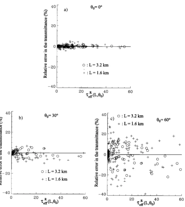
(Figures 8a, 8b, 8c). The relative error is bounded
as ref t increases, because there is a compensation be-
tween
the decreases
of s and re•(6}o
). As expected,
it
is strongly dependent on 6}o, from less than 5% for the
vertical incidence to 7% and 20% for 30 ø and 60 ø when
averaged over L - 1.6 km. Doubling L to 3.2 km brings in only a slight improvement. The variation of the rela- tive error with the averaging scale bears out the MSAv
values proposed in subsection 3.1.2. Indeed, the trans-
mittance can be obtained with a relative error less than
5% for 0 ø _< 6}o _< 30 ø provided that L _> 3.2 kin; this
segment.
Since
T{r[/r•inhom(Z,0o)
,
6}0]}
- T/
inhom(L,0o)-
,
corresponds
to an aspect
ratio of the cloud
segment
s by definition,
the relative
error
can
be expressed
as (aspect
ratio
- horizontal
vertical
thickness)
length
about 10. L >_ 6 km
•_+o o 20 R 40 60 'l;eff (L,00) 4O
• •o
• o ;>.- 20-4{)
[
0o = 30 ø 40o+++•
+ øø
•F + + o' L= 3.2 km +' L= 1.6km,• 20
.E •= o •.-2o 0o = 60 ø + +o%+
++ + o+04• + 0
I
I
]
-40 [
, , ,+ , I
,
0
20 R
q;eff
(L,00)
40
60
0
Z (L,0o)
• 40
60
Figure 8. Effect
of the incidence
angle
on the relative
error
in the transmittance
when
r•(L)
is
used
for
r•[!L).
Incidence
angles:
(a)6}0-
0ø;k(mb!
6}0-
30ø;
(c)6}0-
60
ø.
Horizontal
scale
of
SZCZAP ET AL.' RADIATIVE TRANSFER IN INHOMOGENEOUS NONABSORBANT CLOUDS 20,627
would be required for the same error for 00 - 60 ø. This
means
that r•%
may
introduce
a significant
error
in the
estimation of transmittance, even if the transmittance
is estimated at an aspect ratio of as large as 20.
3.2. Relation Between reft and Local Cloud
Properties
In analyzing the dependency of reft on the local mean optical depth and scale of averaging, we have to use, in principle, only veer estimated for cloud segments with a horizontal extent larger than the MSAv, i.e., a small contribution of s term. However, this would limit con- siderably the scope of the present analysis, because only few veer satisfy such a condition for the 30 ø and 60 ø in- cidences. Hence we considered all %ff estimated fbr the
scales of averaging larger than or equal to 1.6 kin, even
if this results in a larger dispersion.
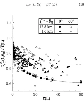
Since %er is a quasi-linear function of 5, we computed the ratio between these two optical depths' r'(L. 00) - •-eer(L, Oo)/5(L), and plotted it as a function of 5. Fig- ure 9 represents r'(L, 0o) computed for two averaging scales, 12.8 km and 1.6 kin,respectively and for two inci- dence angles, 0 ø and 60 ø, respectively. It clearly shows the dependency of r'(L,0o) on the local mean optical depth, but also on the horizontal scale of averaging. The dependency on the scale of averaging occurs because the "degree of inhomogeneity" depends on the averag- ing scale, whatever the exact meaning of the "degree of inhomogeneity" is.
For a large mean optical depth the ratio apt)roaches an asymptotic value 3, so we have approximately
Oo) e (•8) 1.4• [ 1.2
•
0o 60
ø
12.8 km ß o 1.6km • • 0.8o.s
I
I o 6oFigure 9. Variation of r'(L,0o)- %er(L, Oo)/5(L) as a function of the local mean optical depth 5(L); solar
incidence angle: 00 - 0 ø and 00 - 60 ø Horizontal averaging scale' L- 12.8 km and L- 1.6 kin.
This is evident for the 12.8 km averaging, while for 1.6 km, it is much less evident due to a large dispersion of
the estimated ratios. Cahalan et al. [1994a] proposed a
similar expression with a constant coefficient of/3 - 0.7 for an inhomogeneous cloud with a mean optical depth of about 13. For the 12.8 km averaging, r'(L,0o) de- creases from 1.0 at • - 0 to about 0.63 at 5 > 60. We
find 3 -• 0.75 for • - 13, which corresponds approx-
imately to • - 0.7 given by Cahalan et al. Figure 9 shows that %er under the EHCA differs fi'om %ff de- fined under the ETA by more than 20% for small mean optical depth and by more than 10% for large mean
optical depth.
In spite of a larger dispersion we can remark that
the coefficient 3 approaches to 1, on average, as the
scale of averaging decreases. This occurs because the
standard deviation of fluctuations in the optical depth
decreases with the decreasing scale of averaging, due to
the - 1.5 spectral slope of the optical depth fluctuations. When the averaging scale is smaller than the MSAv,
the dispersion of r(L, 00) is quite important because of' a significant variability of local inhomogeneity from one cloud segment to another. Another reason for this large
dispersion is the contribution of the s term, which is due to the nonzero net horizontal photon transport between
the cloud segment and the adjacent cloud pixels. We defined a local relative cloud-inhomogeneity pa-
rameter as p•(L) - cr•(L)/5(L), where cr•(L) and 5(L)
designate, respectively, the local standard deviation of
optical depth fluctuations and the local mean optical
depth over a cloud segment of L . The reason fbr tiffs choice is that as the mean optical depth 5(L) varies,
the same cr•(L) does not have the same eftbet on the radiant flux components, i.e., the reflectance and trans-
mittante of the cloud segments. The square of' this local relative cloud-inhomogeneity parameter is the inverse of
the cloud-inhomogeneity parameter proposed indepen-
dently in the gamma IPA by Barker [1996b 1. However,
its use in this study is significantly different fi'om that
of Barker's work. The present results show that the rel-
ative cloud inhomogeneity is scale-dependent, and this
may have important consequences in analyzing experi-
mental data obtained at different scales of averaging. An empirical relation between reft(L) and 5(L) has
to satisfy the following conditions:
(œ) - (œ) as (œ) -3 0,
7-eft (L) -- e (L) as • (L) -30. (19) The first condition means that when the relative cloud-
inhomogeneity parameter goes down to zero, an inho- mogeneous cloud segment behaves as a homogeneous cloud with the same local mean optical depth. The second condition, independent from the first one, im-
plies that the cloud inhomogeneity should have no ef-
fect when the mean optical depth becomes very small
(Figure 9).
We determined an empirical relation for %ff by fitting the data points to the following function: