Simple measures of ozone depletion in the polar stratosphere

(1)

HAL Id: hal-00302953

https://hal.archives-ouvertes.fr/hal-00302953

Submitted on 6 Jul 2007

HAL is a multi-disciplinary open access

archive for the deposit and dissemination of sci-entific research documents, whether they are pub-lished or not. The documents may come from teaching and research institutions in France or abroad, or from public or private research centers.

L’archive ouverte pluridisciplinaire HAL, est destinée au dépôt et à la diffusion de documents scientifiques de niveau recherche, publiés ou non, émanant des établissements d’enseignement et de recherche français ou étrangers, des laboratoires publics ou privés.

Simple measures of ozone depletion in the polar

stratosphere

R. Müller, J.-U. Grooß, C. Lemmen, D. Heinze, M. Dameris, G. Bodeker

To cite this version:

R. Müller, J.-U. Grooß, C. Lemmen, D. Heinze, M. Dameris, et al.. Simple measures of ozone depletion in the polar stratosphere. Atmospheric Chemistry and Physics Discussions, European Geosciences Union, 2007, 7 (4), pp.9829-9866. �hal-00302953�

(2)

ACPD

7, 9829–9866, 2007 Simple measures of polar ozone depletion

R. M ¨uller Title Page Abstract Introduction Conclusions References Tables Figures ◭ ◮ ◭ ◮ Back Close

Full Screen / Esc

Printer-friendly Version Interactive Discussion

EGU Atmos. Chem. Phys. Discuss., 7, 9829–9866, 2007

www.atmos-chem-phys-discuss.net/7/9829/2007/ © Author(s) 2007. This work is licensed

under a Creative Commons License.

Atmospheric Chemistry and Physics Discussions

Simple measures of ozone depletion in

the polar stratosphere

R. M ¨uller1, J.-U. Grooß1, C. Lemmen1,*, D. Heinze1, M. Dameris2, and G. Bodeker3

1

ICG-1, Forschungszentrum J ¨ulich GmbH, 52425 J ¨ulich, Germany

2

DLR, IPA, Oberpfaffenhofen, Germany

3

NIWA, Private Bag 50061, Omakau Central Otago, New Zealand

*

now at: Copernicus Instituut voor Duurzame Ontwikkeling en Innovatie, Universiteit Utrecht, 3584CS Utrecht, The Netherlands and Institut f ¨ur K ¨ustenforschung,

GKSS-Forschungszentrum Geesthacht GmbH, 21502 Geesthacht, Germany Received: 15 May 2007 – Accepted: 3 July 2007 – Published: 6 July 2007 Correspondence to: R. M ¨uller (ro.mueller@fz-juelich.de)

(3)

ACPD

Full Screen / Esc

EGU

Abstract

We investigate the extent to which commonly considered quantities, based on total col-umn ozone observations and simulations, are applicable as measures of ozone loss in the polar vortices. Such quantities have been used frequently in ozone assessments by the World Meteorological Organization (WMO) and to assess the performance of

5

chemistry-climate models. The most commonly considered quantity is monthly mean column ozone poleward of a latitude of 63◦ in spring. For the Arctic, these monthly means were found to be insensitive to the exact choice of the latitude threshold, unlike the Antarctic where greater sensitivity was found. Choosing a threshold based on the location of the transport barrier at the vortex boundary instead of geometric latitude

10

led to a roughly similar year-to-year variability of the monthly means, but in particular years deviations of several tens of Dobson units occurred. Moreover, the minimum of daily total ozone minima poleward of a particular latitude, another popular measure, is debatable, insofar as it relies on one single measurement or model grid point. For Arctic conditions, this minimum value occurred often in air outside the polar vortex,

15

both in the observations and in a chemistry-climate model. As a result, we recommend that the minimum of daily minima no longer be used when comparing polar ozone loss in observations and models. As a possible alternative, we suggest considering the minimum of daily average total ozone poleward of a particular equivalent latitude (or in the vortex) in spring. This definition both obviates relying on one single data point and

20

reduces the impact of year-to-year variability in the Arctic vortex breakup on ozone loss measures. However, compact relations of such simple measures with meteorological quantities that describe the potential for polar heterogeneous chlorine activation and thus ozone loss were not found. Therefore, we argue that where possible, more so-phisticated measures of chemical polar ozone loss that include additional information

25

(4)

ACPD

Full Screen / Esc

EGU

1 Introduction

Since the early eighties, substantial chemical ozone loss has occurred over winter and spring each year in the Antarctic; (e.g.,Jones and Shanklin,1995;Tilmes et al.,2006; Huck et al.,2007;WMO,2007) substantial chemical loss of ozone has likewise been reported for recent cold Arctic winters (e.g.,Manney et al.,2003;Tilmes et al.,2004;

5

WMO,2007). In the very cold Arctic winter of 2004/05, the chemical loss of ozone came closer to Antarctic values (Manney et al.,2006;Rex et al.,2006;Tilmes et al.,2006; von Hobe et al.,2006;Jin et al.,2006). Sophisticated methods have been developed to separate dynamically induced changes of polar ozone from chemical ozone depletion (e.g., Proffitt et al., 1990; Manney et al.,1994; M ¨uller et al., 1996; Rex et al.,2002;

10

Harris et al., 2002;Christensen et al.,2005;Goutail et al.,2005;Tilmes et al.,2004, and references therein). Furthermore, the deduced chemical ozone loss has been shown to be closely related to the potential for the formation of polar stratospheric clouds (PSC,Rex et al.,2004;Tilmes et al.,2004,2006).

However, these methods rely on rather comprehensive data sets that are not

avail-15

able for all winters of interest, particularly those before the 1990s. Similarly, the neces-sary information for applying such sophisticated methods to simulations conducted with chemistry-climate models (CCM) is often not available for the archived model output (e.g.,Austin et al.,2003;Eyring et al.,2006;Lemmen et al.,2006b).

Therefore, measures of chemical polar ozone depletion are commonly employed that

20

rely solely on total column ozone data (e.g.,Newman et al.,2004;Bodeker et al.,2005; Huck et al.,2007). Such simple measures include the average total column ozone in spring (March, NH and October, SH) poleward of 63◦, or the minimum of daily total column ozone minima over the polar cap (e.g., Newman et al., 1997; M ¨uller, 2003; Austin et al., 2003; WMO,2003;Eyring et al.,2006;WMO, 2007). In particular, the

25

average March total column ozone poleward of 63◦N (Newman et al.,1997) has been used frequently for assessments of the World Meteorological Organization (WMO) and of the Intergovernmental Panel on Climate Change (IPCC, e.g., WMO, 1999, 2003;

(5)

ACPD

Full Screen / Esc

EGU IPCC/TEAP, 2005; WMO, 2007). The value of 63◦N was chosen by Newman et al.

(1997), because “. . . the area poleward of 63◦N is [. . . ] large enough to contain the polar vortex, yet small enough to not be dominated by mid-latitude air masses in the lower stratosphere”. Obviously, this condition will be better fulfilled in some Arctic win-ters than in others depending on the varying size and shape of the polar vortex (Waugh

5

and Randel,1999;Karpetchko et al.,2005).

Moreover, the minimum of daily total ozone minima poleward of a particular latitude has been used as a standard to assess the performance of CCMs (e.g.,Austin et al., 2003; WMO, 2003; Eyring et al., 2006; WMO,2007). This measure is problematic, insofar as it relies on one single measurement or model grid point. Knudsen (2002)

10

has criticised the use of this parameter and pointed out that the minimum ozone in the Arctic is frequently caused by high pressure systems rather than by chemical ozone destruction. He therefore argued that e.g., the March 63◦N–90◦N mean total column ozone should be a more suitable measure for the development of polar ozone.

Here, we scrutinise the information that can be deduced from simple (total column

15

ozone based) measures of chemical ozone loss and investigate circumstances where mis- and over-interpretations might occur. Our study uses a combined data set of satellite-based total column ozone measurements (Bodeker et al.,2005) from 1978 to 2007 (Sect.2). Monthly mean column ozone poleward of 63◦in spring (Newman et al., 1997; WMO,2007) shows similar year-to-year variability as vortex mean ozone, but

20

neither of these quantities shows a close relation with meteorological quantities that describe the potential for polar heterogeneous chlorine activation and thus ozone loss (Sect.3). Furthermore, we argue here that the minimum of daily total ozone minima poleward of a particular latitude should no longer be used when comparing polar ozone loss between observations and CCMs because this minimum value often occurs in air

25

outside of the polar vortex (Sect.3). We discuss alternatives for such simple measures,

both measures based on total ozone observations alone and measures based on more sophisticated techniques.

(6)

ACPD

Full Screen / Esc

EGU

2 The total column ozone data set

The data set used here is version 2.6 of the NIWA combined ozone data base which provides daily total column ozone fields from November 1978 to March 2007. It is based on version 8 TOMS (Total Ozone Mapping Spectrometer) retrievals from four different satellites (Nimbus 7, Meteor 3, ADEOS, and Earth Probe), total column ozone

5

retrievals from application of the TOMS version 8 retrieval algorithm to OMI (Ozone Monitoring Instrument) measurements, version 3.1 GOME (Global Ozone Monitoring Experiment) ozone retrievals, GOME total column ozone fields from the KNMI TO-GOMI algorithm, and version 8 SBUV (Solar Backscatter Ultra-Violet) retrievals from four different satellites (Nimbus 7, NOAA 9, NOAA 11, and NOAA16). It updates the

10

data set described inBodeker et al.(2005), extending it to the end of March 2007, and implementing a number of improvements including:

– Data from both the Dobson spectrophotometer and Brewer spectrometer global networks are now used to remove offsets and drifts between the various satellite-based total column ozone data sets used to construct the data base.

15

– Data from the Ozone Monitoring Instrument (OMI) flown onboard NASA’s Aura satellite since September 2004 are now used. Differences between OMI overpass measurements and ground-based measurements are small (−2.8±5 DU) and the OMI grid data are corrected before they are combined with the other data sources which are also corrected as inBodeker et al.(2005).

20

– A better correction function for the Earth Probe TOMS ozone measurements has been derived to account for non-linearities in the drift between the Earth Probe TOMS measurements and ground-based measurements in recent years. Since September 2004 these data are only used when OMI data are unavailable.

– Better screening of anomalous ozone measurements from the DLR GOME

re-25

(7)

ACPD

Full Screen / Esc

EGU

– In previous versions of the combined database, data from only one satellite-based instrument were used on any given day. In this version of the database, data from all satellite-based instruments are considered sequentially to fill each 1.25◦ longitude by 1.0◦ latitude grid cell with a priority of Nimbus 7 TOMS, Meteor 3 TOMS, OMI, Earth Probe TOMS, ADEOS TOMS, the KNMI and then DLR GOME

5

ozone retrievals, and then the 4 SBUV data sets. For example, if most, but not all, of the globe is covered by Nimbus 7 TOMS and Meteor 3 TOMS data are available to fill the gap, then these data are used for this. Both data sets, as before, are first corrected for offsets and drifts against the ground-based measurements. In previous versions of the data base however, only the Nimbus 7 data would have

10

been used for that day and the gap in the data would remain.

3 Results

3.1 Mean total column ozone over the poles in early spring

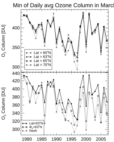
To test the sensitivity of the calculated Arctic mean ozone to the selected latitude limit, the March mean Arctic total column ozone for a latitude boundary at 63◦N, as

origi-15

nally chosen byNewman et al. (1997), is compared with the mean for boundaries at 60◦N, 65◦N, and 70◦N in Fig. 1 (top panel). Clearly, the monthly spatial means are not very sensitive on the exact choice of the threshold latitude. A very similar picture is found for the average total ozone column in April (see electronic supplement). During the eighties, and in the warmer winters during the nineties, choosing a more

pole-20

ward threshold latitude yields greater average ozone columns. The opposite (a smaller ozone column for a more poleward threshold latitude) is observed for the cold Arctic winters 1994/1995, 1995/1996, and 1999/2000 where substantial chemical ozone loss was observed (e.g.,Manney et al.,2003;Tilmes et al.,2004). The strongest effect from changing the threshold latitude is found for the winter 1996/1997, a winter where the

25

(8)

ACPD

Full Screen / Esc

EGU et al.,1997).

Using equivalent latitude (Φ_e) rather than geographic latitude as an estimate of the boundary of the vortex (e.g.,Butchart and Remsberg,1986;Lary et al.,1995), should lead to a better demarcation between polar and mid-latitude air. Therefore, in Fig.1 (bottom panel), the total column ozone average for March in the Arctic is shown using

5

both the latitude and the equivalent latitude poleward of 63◦N as the threshold. Here and throughout the paper equivalent latitude and other diagnostics of the vortex edge are evaluated on the 475 K potential temperature level, except where stated otherwise. Overall the two averages show a similar inter-annual pattern. When equivalent latitude is used as the threshold, Arctic winters with a polar centric vortex (e.g., 1996/1997)

10

show little change, while winters in the nineties with substantial chemical ozone loss within a perturbed vortex show lower averages. This result is not surprising because, when using equivalent latitude as the threshold, the average ozone is less likely to be influenced by air from outside the vortex where, in winters with substantial ozone loss, ozone is higher.

15

An estimate of the location of the vortex boundary, i.e. the location of the strongest barrier to meridional transport in the polar region, and which is based on fluid-dynamical theory, is the maximum gradient in potential vorticity in equivalent latitude constrained by the horizontal wind velocity (Nash et al.,1996). The edge of the vortex defined in this way agrees reasonably well with observed strong tracer gradients at the

20

vortex boundary (e.g., Greenblatt et al.,2002; M ¨uller and G ¨unther, 2003). Because the area of the polar vortex varies substantially from year to year in the Arctic (e.g., Karpetchko et al., 2005; Tilmes et al., 2006), a constant equivalent latitude cannot provide an accurate estimate of the vortex area. Thus, because chemical ozone loss is confined to within the vortex boundary, one expects that the average total column

25

ozone poleward of the vortex edge as defined byNash et al.(1996) should show lower values than an average based on geometric or constant equivalent latitude. This is indeed borne out by the analysis, with the exception of the warm winters of 1978/1979, 1984/1985, 1987/1988, and 1998/1999 (Fig.1, bottom panel). All four of these Arctic

(9)

ACPD

Full Screen / Esc

EGU winters show a very low PSC formation potential and thus a very small potential for

chemical ozone destruction (Rex et al.,2004;Tilmes et al.,2006). For all other win-ters, the polar average total column ozone using a potential vorticity gradient based threshold is lower than using any other threshold and the difference is particularly pro-nounced for winters showing strong ozone depletion. The sole exception is the winter

5

of 1996/1997 that showed an unusually inhomogeneous ozone distribution within the Arctic vortex with a particularly low ozone column in the vortex core (e.g., Newman et al.,1997;Manney et al.,1997;McKenna et al.,2002).

The Arctic vortex, typically, is strongly eroded in April and is therefore smaller than the area encompassed by the 63◦N equivalent latitude contour (e.g., Waugh

10

and Randel, 1999). Consequently, column ozone in April averaged over the vor-tex area as deduced using the Nash et al. (1996) criterion is expected to be lower than the average column ozone poleward of 63◦N equivalent latitude, as is the case here (see electr. suppl., http://www.atmos-chem-phys-discuss.net/7/9829/2007/ acpd-7-9829-2007-supplement.zip). Because the Arctic vortex in April is unlikely to

15

be polar centred, computing a polar average column ozone using geometric latitude rather than equivalent latitude as the threshold, should lead to even more ozone-rich mid-latitude air masses being included in the average, and thus should lead to even greater averages as it is indeed the case (see electr. suppl., http://www. atmos-chem-phys-discuss.net/7/9829/2007/acpd-7-9829-2007-supplement.zip).

20

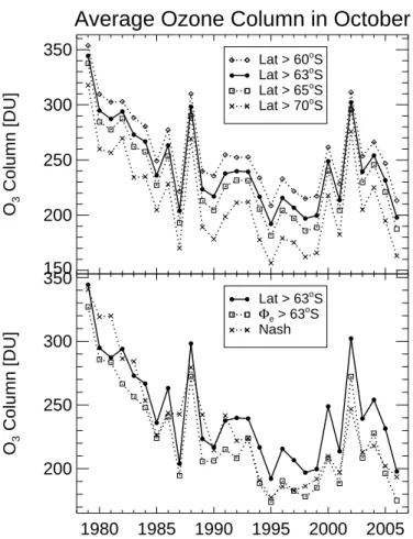
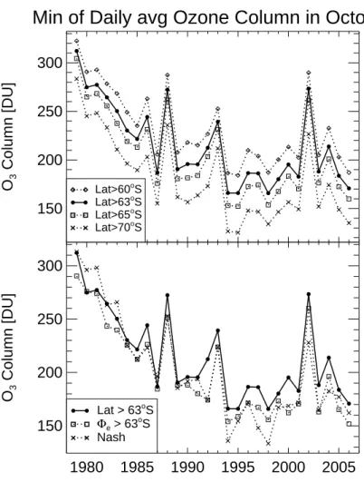
Although originally designed for the Arctic, the concept of the average total ozone column poleward of a threshold latitude of 63◦ has been extended to the Antarctic, where October mean values are commonly considered (e.g.,WMO,1999;IPCC/TEAP, 2005;WMO,2007). In the Antarctic, the choice of the threshold latitude has a much stronger impact on the October average polar column ozone compared to the Arctic;

25

the difference between a threshold of 60◦S and 70◦S is noticeable in every Antarctic winter analysed here and can be as large as ∼50 DU (Fig.2, top panel). The pattern of inter-annual change in the October mean ozone column, however, is not strongly affected by the choice of the threshold latitude. These statements are likewise valid for

(10)

ACPD

Full Screen / Esc

EGU the average total ozone column in September (see electronic supplement). As for the

Arctic, the sensitivity of Antarctic average total column ozone to the latitude poleward of which the average is calculated depends on the steepness of the meridional gradients in ozone across the vortex edge. For the latitude range considered in Fig.2, the ozone gradients are steeper in the Antarctic than the Arctic (see e.g. Fig. 5 ofBrunner et al.

5

2006) and so Antarctic mean total column ozone is expected to be more sensitive to the spatial limiting latitude.

In the Antarctic, the 63◦S equivalent latitude contour is often located within the polar vortex in early spring (e.g., Bodeker et al., 2001, 2002). As a result, the difference between the average column ozone poleward of the Nash defined vortex edge and

10

the average poleward of 63◦S equivalent latitude (Fig.2, bottom panel) is smaller than in the Arctic. Using the Nash vortex edge as the limiting contour for the averaging includes air masses towards the vortex edge that are not included if a threshold of 63◦S equivalent latitude is used. Because total column ozone in the Antarctic vortex increases towards the vortex boundary (Bodeker et al.,2002), using the Nash criterion

15

will generally lead to greater polar total ozone averages (Fig. 2, bottom panel). The only obvious exception to this observation in the October time series analysed here is the winter of 2002. In this winter, at the end of September, a sudden stratospheric warming occurred in the Antarctic vortex, leading to a much smaller and weaker vortex than usual, reminiscent of Arctic conditions (e.g., Kr ¨uger et al., 2005; Newman and

20

Nash,2006).

3.2 Minimum column ozone in the polar region

3.2.1 Minimum polar total column ozone in observations

The minimum of daily total column ozone between 60◦ and the pole for the period March/April in the Arctic and September–November in the Antarctic has been employed

25

as measure of polar ozone loss for the validation of CCMs (Austin et al.,2003;WMO, 2003;Eyring et al.,2006;WMO,2007). The minimum of daily total column ozone used

(11)

ACPD

Full Screen / Esc

EGU in this study is defined as the minimum value of the daily minima over the respective

periods, i.e. one single measurement or one single model grid point within a two month period.

In Fig.3it is shown that for winters with little chemical ozone destruction a substantial fraction of the daily minimum ozone columns occur outside the polar vortex. For half of

5

the winters considered here about 50% of the daily minima occur outside of the vortex. And for only four winters is the fraction of minima occurring outside below 25%.

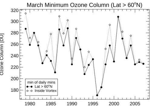
If the minimum value of daily total ozone minima poleward of 60◦N (as used, e.g., in WMO,2003,2007) is computed, it provides information from within the polar vortex in only 12 out of the 29 winters considered here (Fig.4). The deviation between the vortex

10

minimum total ozone and the poleward of 60◦N minimum total ozone is significant, with a maximum deviation of ∼50 DU in the winter of 1984/1985.

In the Antarctic, because of the stronger reduction in column ozone due to chem-ical ozone destruction, the situation is different. For the period considered here, the minimum of daily column ozone between 60◦S and the pole for the period

September-15

November (not shown) is always located within the vortex. 3.2.2 Minimum column polar ozone in model results

Differences between different simple measures of ozone loss and between simple and more sophisticated analyses also occur when analysing results from model simula-tions, as will be shown below. Since the prediction of the recovery of polar ozone

20

is based on simulations with CCMs (e.g. Austin et al.,2003; WMO, 2003,2007), the identification of a recovery period may depend on the analysis methodology chosen for ozone loss. In the last two ozone assessments (WMO, 2003,2007) the spatial mini-mum of the daily spring ozone minimini-mum poleward of 60◦served as a quantifier for the state of the polar ozone layer for comparison with simulations from different CCMs.

25

For simulated ozone columns, here, we use as an example two time slice experi-ments from the chemistry-climate model ECHAM4.DLR(L39)/CHEM (hereafter abbre-viated as E39/CHein et al.,2001;Schnadt et al.,2002). Each ensemble experiment

(12)

ACPD

Full Screen / Esc

EGU consists of 20 recurrent simulations with constant boundary conditions (sea surface

temperature, greenhouse gases), one for the 1990s and one for the near-future. The near-future conditions originally aimed at the year 2015, but in the interim it has been found that the sea surface temperatures used are too high. Therefore, results from the future simulation should not be considered as a reliable projection of a specific period

5

but rather as being indicative of possible future conditions. The 1990 time slice results, in contrast, are in agreement with the results derived from the most recent transient ensemble run for 1960 to 1999 (Dameris et al.,2005;Eyring et al.,2006). A detailed description of both time slice experiments and the simulation of ozone therewith is given elsewhere (Schnadt,2001;Lemmen,2005).

10

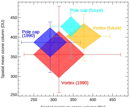
Figure5compares ensemble statistics of both time slices analysed separately for the polar cap and the dynamically defined vortex, all data reported for April 1. For example, in the 1990 simulation poleward of 60◦N (dark blue colour), the spatial mean ozone column (ordinate) was 387 DU and the range was 310–439 DU. In half of the years, the spatial mean column was larger than 403 DU. For the same analysis, the mean

15

and range of the spatial minimum column (abscissa) are 291 DU and 218–369 DU. Column values for ‘future’ (cyan, dark yellow) are consistently higher than for ‘1990’ (blue, red) due to a lower chlorine loading and more dynamical heating leading to a stronger downward transport (Schnadt et al.,2002;Eyring et al.,2006).

For both time slices, the spatial mean total column ozone is higher over the polar

20

cap than over the vortex, and the spatial minimum column is lower over the polar cap than over the vortex; this difference in spatial analysis is more pronounced in the future experiment (with less chemical ozone destruction). For the 1990 experiment, 50% of the years have a minimum column less than 310 DU analysed within the vortex, but 75% of these winters have a minimum column less than 310 DU analysed within the

25

polar cap. Evidently, for many years the spatial minimum is located outside the vortex in spite of the on average lower ozone column within the vortex.

The erroneous association of the spatial minimum column ozone with high chemical ozone loss becomes clear in a comparison with analysed chemical ozone loss.

(13)

Chemi-ACPD

Full Screen / Esc

EGU cal ozone loss based on a methane-ozone tracer correlation with reference established

on 1 January each simulated year and compared to the 1 April methane-ozone rela-tion was first presented by Lemmen (2005) for this data set. Here, the loss values are recalculated based on an improved method to determine the vortex edge. The vortex edge was determined by fitting a third-order polynomial to the potential vorticity

5

(PV) distribution as a function of Φ_efor each potential temperature level between 340– 640 K, defining the vortex edge by the steepest PV gradient constrained by the wind maximum on each level, converting the PV value at the vortex boundary to modified PV (Lait,1994), and then using the median of these modified PV values as the criterion for distinguishing between vortex and out-of-vortex air masses in the model. The ozone

10

column and vortex data for individual years of both time slice experiments are given in the online supplement (timeslice column.tsv).

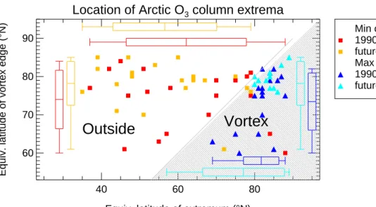
For both time slices, Fig. 6 relates the location (in equivalent latitude) of the mini-mum ozone column and the maximini-mum chemical ozone column loss to the location of the vortex edge as defined by Nash et al. (1996). For all winters of both time slice

15

experiments, the maximum chemical column ozone loss is located within (or, in two cases, on) the polar vortex edge, i.e., in the shaded region in Fig. 6. For only three winters in each time slice experiment is the polar cap ozone minimum located within the vortex. On the ensemble average (determined separately for each time slice, un-certainty given as one standard deviation), the vortex edge is located at Φ_e≈74◦±8◦ in

20

1990 (78◦±6◦ for “future”), and the location of the polar cap minimum around 62◦±15◦ (57◦±13◦), i.e., clearly outside of the vortex.

Arguably, the simulated vortex area, Φ_e>74◦ on 1 April for many of the analysed winters, is smaller than observed climatological Arctic vortex areas (e.g.,Karpetchko et al.,2005, report Φ_e≈69◦ for the climatological Arctic vortex edge). The remaining

25

vortex possibly does not encompass all chemically depleted air masses at this time anymore. Still, even when a generous vortex boundary definition such as Φ_e=₆₃◦ _is considered, for more than half of all winters the polar cap minimum ozone is located outside this rather generously defined vortex.

(14)

ACPD

Full Screen / Esc

EGU Lemmen et al.(2006b) recommended that a more sophisticated measure should be

applied to CCM simulations to isolate chemical (halogen-induced) ozone loss from to-tal ozone change; they suggested using tracer-tracer correlations (TRAC) (e.g.,Proffitt et al.,1990;Tilmes et al.,2004;M ¨uller et al.,2005). They demonstrated their applica-bility to output from a model simulation (Lemmen et al.,2006b) and employed TRAC

5

on a recent 40-year transient CCM simulation (Lemmen et al.,2006a).

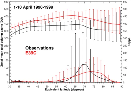
The fact that the size of the Arctic vortex in E39/C is smaller than in reality is high-lighted in Fig.7 where the strength of the barrier to meridional transport (κ=∇PV·v, where v is the absolute value of the horizontal wind velocity,Bodeker et al.,2001) is compared with the same quantity calculated using output from the transient run with

10

E39/C (Dameris et al.,2005) as a function of equivalent latitude on the 550 K surface. Observed potential vorticity and wind fields on the 550 K surface were obtained every 6 hours from the NCEP/NCAR reanalysis data base for these calculations. We focus on the first ten days of April to avoid too much sampling of vortex break downs which are more likely to occur towards the end of April and on the years 1990–1999 to focus

15

on the period when ozone depletion over the Arctic maximises. Clearly the dynamical vortex in E39/C is weaker and broader than in reality and leans poleward. As a result, moving poleward in E39/C, ozone decreases more slowly than in reality. Furthermore, the dynamical vortex in the Arctic, as inferred from the maximum in κ would be smaller in area in E39/C (at Φ_e≈73◦) than in reality (at Φ_e≈69◦,Karpetchko et al.,2005).

20

A similar result is reported by Tilmes et al. (2007a)1for the WACCM3 model, where the maximum of κ in the Arctic is smaller in magnitude and located further poleward with a much wider peak compared to observations.

1

Tilmes, S., Kinnisen, D., M ¨uller, R., Sassi, F., Marsh, D., Boville, B., and Garcia, R.: Eval-uation of heterogeneous processes in the polar lower stratosphere in WACCM3, J. Geophys. Res., submitted, 2007.

(15)

ACPD

Full Screen / Esc

EGU 3.2.3 Minimum of the daily average column ozone

As an alternative measure for the maximum chemical impact on column ozone over the polar region, we suggest that the daily mean area weighted ozone over the polar region should be considered and then that the minimum value reached in March in the Arctic and in October in the Antarctic should be selected. This value should approximately

5

reflect the maximum impact of chemical loss on the ozone column before the vortex breaks down or before substantial mixing into the vortex occurs. The time series of this quantity for March in the Arctic (Fig. 8) shows substantial year-to-year variation, with values below 350 DU reached in several years. Generally, the lowest values are reached if ozone is averaged over the polar vortex (with the edge determined from the

10

gradient in PV (Nash et al., 1996) on the 475 K potential temperature level) and the greatest values if the average is taken poleward of 63◦N. Averages taken poleward of an equivalent latitude of 63◦N range between the two extremes. This indicates that throughout the period considered, column ozone is generally lower within the boundary of the Arctic vortex than outside.

15

The minimum daily average polar ozone in October in the Antarctic (Fig. 9) shows less year-to-year variability and clearly lower ozone values than in the Arctic. All values after 1980 are lower than 300 DU and a decline of the values between ∼1980 and 1995 is noticeable. Compared to the Arctic, there is less variation in this quantity depending on whether latitude/equivalent latitude of 63◦S or the vortex boundary is

20

chosen as the limit of the region over which averages are calculated. This observation is consistent with the Antarctic vortex being approximately polar concentric and with a vortex boundary close to 63◦S (e.g.,Bodeker et al.,2002;Karpetchko et al.,2005).

3.3 Relation between the mean polar ozone column and meteorological conditions

In the Arctic, chemical ozone loss is closely related to the particular meteorological

25

conditions in each year. Rex et al.(2004) reported that Arctic chemical loss is linearly related to a measure of the likelihood of polar stratospheric cloud occurrence referred

(16)

ACPD

Full Screen / Esc

EGU to as V_PSC. V_PSC is defined as the volume of stratospheric air below the threshold

temperature for the existence of nitric acid trihydrate, averaged over a certain period and altitude range (Rex et al.,2004). Tilmes et al.(2006) have extended this analysis to Antarctic conditions, introducing the PSC Formation Potential of the polar vortex (PFP). PFP2is a similar measure as V_PSC, but takes into account the size of the vortex. Here

5

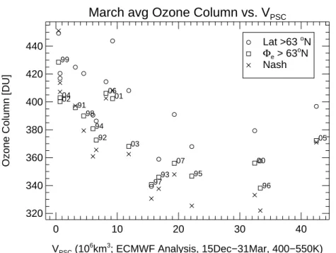
we investigate whether the simple measures of polar ozone loss discussed above show any relation to the measures of chlorine activation in the vortex such as V_PSCand PFP. Figure10 shows a scatterplot of V_PSC against the average column ozone poleward of geometric or equivalent latitude 63◦N and within the vortex. Obviously, in contrast to the compact relation between V_PSCand chemical ozone loss (Rex et al.,2004;Tilmes

10

et al.,2004), there is no close relation between V_PSCand March average ozone. This holds irrespective of the horizontal boundary specified as the limit for the averaging. Apparently, the March average ozone is a measure that does not adequately differ-entiate between chemical loss and dynamical resupply of ozone that both change substantially from year to year. Furthermore, the March average ozone poleward of

15

geometric latitude of 63◦N is particularly sensitive to the strong year-to-year variability in the lifetime and shape of the Arctic vortex (Waugh and Randel, 1999;Karpetchko et al.,2005).

We argued above that the minimum of March daily average polar column ozone should be a quantity more closely related to chemical ozone loss than those shown in

20

Fig. 10. Thus one might expect that the minimum of March average ozone shows a more compact relation with V_PSC. The minimum of daily average ozone when plotted against V_PSC(Fig.11) indeed shows a certain structure, especially, when vortex aver-ages or averaver-ages poleward of 63◦N equivalent latitude are considered. However, there is no clearly compact and especially no linear relation of this quantity with V_PSC.

25

2

PFP is calculated in the following way. For all days when a vortex exists and for a defined altitude range, VPSC is divided by the volume of the polar vortex, and these values are then

integrated over a defined time period. Finally this value is divided by the total number of days in the period (Tilmes et al.,2006).

(17)

ACPD

Full Screen / Esc

EGU Some outliers, e.g. the years 1999, 2001, and 2006 can be understood. For these

years, the final warming was very early such that no vortex existed during March, with the consequence of a larger ozone column caused by the influx of mid-latitude ozone-rich air. Concentrating on data for the years when the polar vortex in March was intact, we find a tighter relation between V_PSCand the minimum of daily average

5

ozone column poleward of Φ_e=₆₃◦_{that is indicated by the dotted line in Fig.}₁₁_{. From} the three different quantities shown, the polynomial fit with this quantity has the lowest deviation (1σ=5.5 DU) from the observations and shows (nearly) monotonic decrease with increasing V_PSC.

When PSC occurrence or the potential for chlorine activation is compared for the

10

Arctic and Antarctic, V_PSC is no longer a suitable measure, because the polar vortex is much larger in the Antarctic than in the Arctic; for such a comparison, the PFP should be used instead of V_PSC(Tilmes et al.,2006). In Fig.12, PFP is plotted against the minimum of March daily average polar column ozone, where only data points for averages poleward of 63◦ equivalent latitude are shown. The well known fact that

15

PFP is larger in the Antarctic than in the Arctic (Tilmes et al., 2006) and that polar column ozone is greater in the Arctic than in the Antarctic (Dobson,1968;WMO,2007) are reflected in this plot. However, for this combination of meteorological and ozone measures, again no clearly compact relation emerges.

4 Discussion

20

Among the quantities describing stratospheric ozone, total column ozone is the one most easily measured. Indeed, the longest atmospheric time series exist for total ozone (e.g.,Staehelin et al.,1998;Br ¨onnimann et al.,2003) and the Antarctic ozone hole was discovered, and the discovery corroborated, through measurements of total column ozone (Chubachi,1984;Farman et al.,1985;Stolarski et al.,1986). However,

25

variations in total ozone are caused by both chemical change and by transport, and the different impact of these processes is often difficult to disentangle.

(18)

ACPD

Full Screen / Esc

EGU Transport contributions to polar ozone variability are closely controlled by the

strength of the middle atmospheric (Brewer-Dobson) circulation that is driven by tropo-spheric wave forcing. For both the Arctic and Antarctic, a stronger-than-average plan-etary wave forcing in winter leads to more transport of ozone to high latitudes because of a stronger circulation and a higher-than-average polar lower stratospheric

temper-5

ature and a weaker vortex in early spring, whereas a weaker wave forcing leads to less transport, lower polar temperatures in spring and to a stronger vortex (Fusco and Salby,1999;Newman et al.,2001;Weber et al.,2003). The variability in polar ozone due to the variability in wave forcing is much larger in the Arctic than in the Antarctic, while chemical loss is more persistent in Antarctica.

10

Here we argue that measures of chemical ozone loss based on monthly averages of total column ozone over the polar cap, although they contain information about chemi-cal ozone loss, must be interpreted with caution. The particular value of such measures will depend on the selected definition of the equatorward boundary of the region over which averages are calculated. In the Arctic, the year-to-year variability of the size of

15

the polar vortex has a particularly strong impact. Averages over the polar cap do not show compact relationships with meteorological measures of the extent of chlorine ac-tivation (and thus the potential for ozone destruction) in the polar vortices such as V_PSC and PFP.

Although frequently employed, the minimum value of daily total column ozone

min-20

ima over the polar region is a particularly problematic measure, insofar as it relies on a single measurement or on a single model grid point. We have shown here that for the Arctic, both in a CCM and in observations, that a significant fraction of the mini-mum values of daily total ozone minima occur outside the polar vortex. Clearly, if the minimum ozone value on a particular day occurs outside the vortex, it does not provide

25

information on halogen driven chemical ozone loss initiated by heterogeneous chlorine activation. Because of the strong chemical ozone loss in the Antarctic, this problem is much less pronounced there. It should, however, become increasingly relevant for sim-ulations of future ozone loss, when much less chemical ozone loss is expected. Based

(19)

ACPD

Full Screen / Esc

EGU on this analysis we must question the applicability of a simple measure such as a

min-imum polar cap ozone value for both the E39/C model and observations, and strongly caution against application of this simple measure to results from other CCM simula-tions. It is remarkable that there is substantial variation in the magnitude of minimum total column ozone in current model simulations ranging roughly from 220 to 320 DU

5

whereas the observations lie in the range of 290 DU to below 200 DU (WMO,2007, Fig. 6–13).

Clearly, employing sophisticated measures of polar chemical ozone loss that show a compact correlation with meteorological measures of chlorine activation (Rex et al., 2004;Tilmes et al.,2006) is the best method to assess the temporal evolution of polar

10

ozone loss in both models and observations. However, when only total column ozone data are available, we propose that the minimum of March average total ozone in the vortex (where the vortex boundary could be determined by the maximum gradient in PV or by an equivalent latitude criterion) should be considered. This quantity is not strongly influenced by low column ozone outside the vortex and does not rely on a

15

single measurement or model grid point. Further, in contrast to monthly averages, its year-to-year variability is not substantially affected by varying dates of vortex break-down in the Arctic.

5 Conclusions

Quantities deduced from measurements of total column ozone are frequently used as

20

measures of polar ozone loss. One of the common measures is monthly mean column ozone poleward of 63◦ for March and October in the Arctic and Antarctic, respectively. For the Arctic, a latitude of 63◦ is a reasonable boundary for polar air, whereas for the Antarctic the values of the October means (but not their year-to-year variability) are sensitive to the exact choice of 63◦. A better definition of the polar vortex boundary can

25

be obtained using the gradient in PV (Nash et al.,1996) or equivalent latitude, however, under no circumstances can a close relation of such simple measures be obtained with

(20)

ACPD

Full Screen / Esc

EGU meteorological quantities that describe the potential for polar heterogeneous chlorine

activation (and thus ozone loss).

The minimum of daily total ozone minima poleward of a particular latitude is a prob-lematic measure, insofar as it relies on one single measurement or on one single model grid point; for Arctic conditions, it is not unlikely that this minimum value occurs in air

5

outside the polar vortex. We suggest that this concept should no longer be used when comparing polar ozone loss in observations and models.

Considering the minimum of daily average total ozone poleward of a particular equiv-alent latitude (or in the vortex) in spring, avoids the problem of relying on one single data point and reduces the impact of year-to-year variability in the Arctic vortex breakup

10

on ozone loss measures. We propose this measure as a candidate for a useful simple measure of polar ozone loss. In any event, it is preferable to employ more sophis-ticated measures of chemical polar ozone loss (e.g., Harris et al., 2002; Rex et al., 2004;Tilmes et al.,2006;Lemmen et al.,2006b;WMO,2007) that bring in additional information to disentangle the transport and the chemical impact on ozone.

15

Acknowledgements. We are grateful to S. Tilmes for helpful discussions on the manuscript and

for providing the values for PFP used here. C. Lemmen was partly supported by the Dutch Envi-ronmental Assessment Agency (Milieu- en Natuurplanbureau Bilthoven, The Netherlands). We thank the European Centre for Medium-Range Weather Forecasts and the UK Meteorological Office for providing meteorological analyses.

20

References

Austin, J., Shindell, D., Beagley, S. R., Br ¨uhl, C., Dameris, M., Manzini, E., Nagashima, T., Newman, P., Pawson, S., Pitari, G., Rozanov, E., Schnadt, C., and Shepherd, T. G.: Uncer-tainties and assessments of chemistry-climate models of the stratosphere, Atmos. Chem. Phys., 3, 1–27, 2003,

25

http://www.atmos-chem-phys.net/3/1/2003/. 9831,9832,9837,9838

(21)

ACPD

Full Screen / Esc

EGU

coordinates using TOMS and GOME intercompared against the Dobson network: 1978-1998, J. Geophys. Res., 106, 23 029–23 042, 2001. 9837,9841

Bodeker, G., Struthers, H., and Connor, B.: Dynamical containment of Antarctic ozone deple-tion, Geophys. Res. Lett., 29, 1098, doi:10.1029/2001GL014206, 2002.9837,9842

Bodeker, G. E., Shiona, H., and Eskes, H.: Indicators of Antarctic ozone depletion, Atmos.

5

Chem. Phys., 5, 2603–2615, 2005,

http://www.atmos-chem-phys.net/5/2603/2005/. 9831,9832,9833

Br ¨onnimann, S., Staehelin, J., Farmer, S., Svendby, T., and Svenøe, T.: Total ozone observa-tions prior to the IGY. I: A history, Q. J. R. Meteorol. Soc., 129, 2797–2817, 2003. 9844

Brunner, D., Staehelin, J., K ¨unsch, H.-R., and Bodeker, G.: A Kalman filter reconstruction

10

of the vertical ozone distribution in an equivalent latitude-potential temperature framework from TOMS/GOME/SBUV total ozone observations, J. Geophys. Res., 111, D12308, doi: 10.1029/2005JD006279, 2006. 9837

Butchart, N. and Remsberg, E. E.: The area of the stratospheric polar vortex as a diagnostic for tracer transport on an isentropic surface, J. Atmos. Sci., 43, 1319–1339, 1986.9835 15

Christensen, T., Knudsen, B. M., Streibel, M., Anderson, S. B., Benesova, A., Braathen, G., Davies, J., Backer, H., Dorokhov, H. D. V., Gerding, M., Gil, M., Henchoz, B., Kelder, H., Kivi, R., Kyr ¨o, E., Litynska, Moore, D., Peters, G., Skrivankova, P., St ¨ubi, R., Turunen, T., Vaughan, G., Viatte, P., Vik, A. F., von der Gathen, P., and Zaitcev, I.: Vortex-averaged Arctic ozone depletion in the winter 2002/2003, Atmos. Chem. Phys., 5, 131–138, 2005,

20

http://www.atmos-chem-phys.net/5/131/2005/. 9831

Chubachi, S.: Preliminary result of ozone observations at Syowa station from February 1982 to January 1983, Mem. Natl. Inst. Polar Res. Spec. Issue, 34, 13–19, 1984. 9844

Dameris, M., Grewe, V., Ponater, M., Deckert, R., Eyring, V., Mager, F., Matthes, S., Schnadt, C., Stenke, A., Steil, B., Br ¨uhl, C., and Giorgetta, M. A.: Long-term changes and variability

25

in a transient simulation with a chemistry-climate model employing realistic forcing, Atmos. Chem. Phys., 5, 2121–2145, 2005,

http://www.atmos-chem-phys.net/5/2121/2005/. 9839,9841,9861

Dobson, G. M. B.: Forty years’ research on atmospheric ozone at Oxford: a history, Appl. Opt., 7, 387–405, 1968. 9844

30

Eyring, V., Butchart, N., Waugh, D. W., Akiyoshi, H., Austin, J., Bekki, S., Bodeker, G. E., Boville, B. A., Br ¨uhl, C., Chipperfield, M. P., Cordero, E., Dameris, M., Deushi, M., Fioletov, V. E., Frith, S. M., Garcia, R. R., Gettelman, A., Giorgetta, M. A., Grewe, V., Jourdain,

(22)

ACPD

Full Screen / Esc

EGU

L., Kinnison, D. E., Mancini, E., Manzini, E., Marchand, M., Marsh, D. R., Nagashima, T., Nielsen, E., Newman, P. A., Pawson, S., Pitari, G., Plummer, D. A., Rozanov, E., Schraner, M., Shepherd, T. G., Shibata, K., Stolarski, R. S., Struthers, H., Tian, W., and Yoshiki, M.: Assessment of temperature, trace species and ozone in chemistry-climate simulations of the recent past, J. Geophys. Res., 111, D22308, doi:10.1029/2006JD007327, 2006.9831,9832,

5

9837,9839

Farman, J. C., Gardiner, B. G., and Shanklin, J. D.: Large losses of total ozone in Antarctica reveal seasonal ClOx/NOxinteraction, Nature, 315, 207–210, 1985. 9844

Fusco, A. and Salby, M.: Interannual variations of total ozone and their relationship to variations of planetary wave activity, J. Climate, 12, 1619–1629, 1999.9845

10

Goutail, F., Pommereau, J.-P., Lef `evre, F., Roozendael, M. V., Andersen, S. B., K ˚astad-Høiskar, B.-A., Dorokhov, V., Kyr ¨o, E., Chipperfield, M. P., and Feng, W.: Early unusual ozone loss during the Arctic winter 2002/2003 compared to other winters, Atmos. Chem. Phys., 5, 665– 677, 2005,

http://www.atmos-chem-phys.net/5/665/2005/. 9831 15

Greenblatt, J. B., Jost, H.-J., Loewenstein, M., Podolske, J. R., Bui, T. P., Hurst, D. F., Elkins, J. W., Herman, R. L., Webster, C. R., Schauffler, S. M., Atlas, E. L., Newman, P. A., Lait, L. L., M ¨uller, M., Engel, A., and Schmidt, U.: Defining the polar vortex edge from an N2O:potential

temperature correlation, J. Geophys. Res., 107, 8268, doi:10.1029/2001JD000575, 2002.

9835 20

Harris, N. R., Rex, M., Goutail, F., Knudsen, B. M., Manney, G. L., M ¨uller, R., and von der Ga-then, P.: Comparison of empirically derived ozone loss rates in the Arctic vortex, J. Geophys. Res., 107, 8264, doi:10.1029/2001JD000482, 2002. 9831,9847

Hein, R., Dameris, M., Schnadt, C., Land, C., Grewe, V., K ¨ohler, I., Ponater, M., Sausen, R., Steil, B., Landgraf, J., and Br ¨uhl, C.: Results of an interactively coupled atmospheric

25

chemistry-general circulation model: Comparison with observations, Ann. Geophys., 19, 435–457, 2001,

http://www.ann-geophys.net/19/435/2001/. 9838

Huck, P., Tilmes, S., Randel, W., McDonald, A., and Nakajima, H.: An Improved measure for ozone depletion in the Antarctic stratosphere, J. Geophys. Res., accepted, doi:10.1029/XX,

30

2007. 9831

IPCC/TEAP: Special Report on Safeguarding the Ozone Layer and the Global Climate System: Issues Related to Hydrofluorocarbons and Perfluorocarbons, Cambridge University Press,

(23)

ACPD

Full Screen / Esc

EGU

Cambridge, United Kingdom and New York, NY, USA, edited by B. Metz, L. Kuijpers, S. Solomon, S. O. Andersen, O. Davidson, J. Pons, D. de Jager, T. Kestin, M. Manning and L. Meyer, 2005. 9832,9836

Jin, J. J., Semeniuk, K., Manney, G. L., Jonsson, A. I., Beagley, S. R., McConnell, J. C., Dufour, G., Nassar, R., Boone, C. D., Walker, K. A., Bernath, P. F., and Rinsland, C. P.: Severe Arctic

5

ozone loss in the winter 2004/2005: observations from ACE-FTS, Geophys. Res. Lett., 33, D15801, doi:10.1029/2006GL026752, 2006. 9831

Jones, A. E. and Shanklin, J. D.: Continued decline of total ozone over Halley, Antarctica since 1985, Nature, 376, 409–411, 1995.9831

Karpetchko, A., Kyr ¨o, E., and Knudsen, B.: Arctic and Antarctic polar vortices 1957-2002

10

as seen from the ERA-40 reanalyses, J. Geophys. Res., 110, D21109, doi:10.1029/ 2005JD006113, 2005. 9832,9835,9840,9841,9842,9843

Knudsen, B. M.: Interactive comment on “Uncertainties and assessments of chemistry-climate models of the stratosphere” by J. Austin et al., Atmos. Chem. Phys. Discuss., 2, S323–S324, 2002. 9832

15

Kr ¨uger, K., Naujokat, B., and Labitzke, K.: The unusual midwinter warming in the southern hemisphere stratosphere 2002: A Comparison to northern hemisphere phenomena, J. At-mos. Sci., 62, 603–613, 2005. 9837

Lait, L. R.: An alternative form for potential vorticity, J. Atmos. Sci., 51, 1754–1759, 1994.9840

Lary, D. J., Chipperfield, M. P., Pyle, J. A., Norton, W. A., and Riishøjgaard, L. P.:

Three-20

dimensional tracer initialization and general diagnostics using equivalent PV latitude-potential-temperature coordinates, Q. J. R. Meteorol. Soc., 121, 187–210, 1995. 9835

Lemmen, C.: Future polar ozone: predictions of Arctic ozone recovery in a changing climate, Dissertation, Bergische Universit ¨at Wuppertal, 2005.9839,9840

Lemmen, C., Dameris, M., M ¨uller, R., and Riese, M.: Chemical ozone loss in a

chemistry-25

climate model from 1960 to 1999, Geophys. Res. Lett., 33, L15820, doi:10.1029/ 2006GL026939, 2006a. 9841

Lemmen, C., M ¨uller, R., Konopka, P., and Dameris, M.: Critique of the Tracer-tracer correlation technique and its potential to analyse polar ozone loss in chemistry-climate models, J. Geo-phys. Res., 111, D18307, doi:10.1029/2006JD007298, 2006b.9831,9840,9841,9847 30

Manney, G., Santee, M., Froidevaux, L., Hoppel, K., Livesey, N., and Waters, J.: EOS MLS observations of ozone loss in the 2004-2005 Arctic winter, Geophys. Res. Lett., 33, L04802, doi:10.1029/2005GL024494, 2006. 9831

(24)

ACPD

Full Screen / Esc

EGU

Manney, G. L., Froidevaux, L., Waters, J. W., Zurek, R. W., Read, W. G., Elson, L. S., Kumer, J. B., Mergenthaler, J. L., Roche, A. E., O’Neill, A., Harwood, R. S., MacKenzie, I., and Swinbank, R.: Chemical depletion of ozone in the Arctic lower stratosphere during winter 1992-93, Nature, 370, 429–434, 1994. 9831

Manney, G. L., Froidevaux, L., Santee, M. L., Zurek, R. W., and Waters, J. W.: MLS

ob-5

servations of Arctic ozone loss in 1996-97, Geophys. Res. Lett., 24, 2697–2700, doi: 10.1029/97GL52827, 1997. 9836

Manney, G. L., Froidevaux, L., Santee, M. L., Livesey, N. J., Sabutis, J. L., and Waters, J. W.: Variability of ozone loss during Arctic winter (1991 to 2000) estimated from UARS Microwave Limb Sounder measurements, J. Geophys. Res., 108, doi:10.1029/2002JD002634, 2003.

10

9831,9834

McKenna, D. S., Grooß, J.-U., G ¨unther, G., Konopka, P., M ¨uller, R., Carver, G., and Sasano, Y.: A new Chemical Lagrangian Model of the Stratosphere (CLaMS): 2. Formulation of chemistry scheme and initialization, J. Geophys. Res., 107, 4256, doi:10.1029/2000JD000113, 2002.

9836 15

M ¨uller, R.: Impact of cosmic rays on stratospheric chlorine chemistry and ozone depletion, Phys. Rev. Lett., 91, 058 502, 2003. 9831

M ¨uller, R. and G ¨unther, G.: A generalized form of Lait’s modified potential vorticity, J. Atmos. Sci., 60, 2229–2237, 2003.9835

M ¨uller, R., Crutzen, P. J., Grooß, J.-U., Br ¨uhl, C., Russel III, J. M., and Tuck, A. F.: Chlorine

20

activation and ozone depletion in the Arctic vortex: Observations by the Halogen Occultation Experiment on the Upper Atmosphere Research Satellite, J. Geophys. Res., 101, 12 531– 12 554, 1996.9831

M ¨uller, R., Tilmes, S., Konopka, P., Grooß, J.-U., and Jost, H.-J.: Impact of mixing and chemical change on ozone-tracer relations in the polar vortex, Atmos. Chem. Phys., 5, 3139–3151,

25

2005,

http://www.atmos-chem-phys.net/5/3139/2005/. 9841

Nash, E. R., Newman, P. A., Rosenfield, J. E., and Schoeberl, M. R.: An objective determination of the polar vortex using Ertel’s potential vorticity, J. Geophys. Res., 101, 9471–9478, 1996.

9835,9836,9840,9842,9846,9857,9858,9859 30

Newman, P. A. and Nash, E. R.: The unusual southern hemisphere stratosphere winter of 2002, J. Atmos. Sci., 62, 614–628, 2006.9837

(25)

ACPD

Full Screen / Esc

EGU

Arctic, Geophys. Res. Lett., 24, 2689–2692, doi:10.1029/97GL52381, 1997. 9831, 9832,

9834,9836

Newman, P. A., Nash, E. R., and Rosenfield, J. E.: What controls the temperature of the Arctic stratosphere during the spring?, J. Geophys. Res., 106, 19 999–20 010, doi:10.1029/ 2000JD000061, 2001. 9845

5

Newman, P. A., Kawa, S. R., and Nash, E. R.: On the size of the Antarctic ozone hole, Geophys. Res. Lett., 31, L21104, doi:10.1029/2004GL020596, 2004. 9831

Proffitt, M. H., Margitan, J. J., Kelly, K. K., Loewenstein, M., Podolske, J. R., and Chan, K. R.: Ozone loss in the Arctic polar vortex inferred from high altitude aircraft measurements, Na-ture, 347, 31–36, 1990. 9831,9841

10

Rex, M., Salawitch, R. J., Harris, N. R. P., von der Gathen, P., Schulz, G. O. B. A., Deckelman, H., Chipperfield, M., Sinnhuber, B.-M., Reimer, E., Alfier, R., Bevilacqua, R., Hoppel, K., Fromm, M., Lumpe, J., K üllmann, H., Kleinb öhl, A., von K önig, H. B. M., K ünzi, K., Toohey, D., V ömel, H., Richard, E., Aiken, K., Jost, H., Greenblatt, J. B., Loewenstein, M., Podolske, J. R., Webster, C. R., Flesch, G. J., Scott, D. C., Herman, R. L., Elkins, J. W., Ray, E. A.,

15

Moore, F. L., Hurst, D. F., Romanshkin, P., Toon, G. C., Sen, B., Margitan, J. J., Wennberg, P., Neuber, R., Allart, M., Bojkov, B. R., Claude, H., Davies, J., Davies, W., De Backer, H., Dier, H., Dorokhov, V., Fast, H., Kondo, Y., Kyr ¨o, E., Litynska, Z., Mikkelsen, I. S., Molyneux, M. J., Moran, E., Nagai, T., Nakane, H., Parrondo, C., Ravegnani, F., Viatte, P. S. P., and Yushkov, V.: Chemical depletion of Arctic ozone in winter 1999/2000, J. Geophys. Res., 107,

20

8276, doi:10.1029/2001JD000533, 2002. 9831

Rex, M., Salawitch, R. J., von der Gathen, P., Harris, N. R., Chipperfield, M. P., and Naujokat, B.: Arctic ozone loss and climate change, Geophys. Res. Lett., 31, doi:10.1029/2003GL018844, 2004. 9831,9836,9842,9843,9846,9847

Rex, M., Salawitch, R., Deckelmann, H., von der Gathen, P., Harris, N., Chipperfield, M.,

Nau-25

jokat, B., Reimer, E., Allaart, M., Andersen, S., Bevilacqua, R., Braathen, G., Claude, H., Davies, J., Backer, H. D., Dier, H., Dorokov, V., Fast, H., Gerding, M., Godin-Beekmann, S., Hoppel, K., Johnson, B., Kyr ¨o, E., Litynska, Z., Moore, D., Nakane, H., Parrondo, M., Ris-ley, A., Jr., Skrivankova, P., St ¨ubi, R., Viatte, P., Yushkov, V., and Zerefos, C.: Arctic winter 2005: Implications for stratospheric ozone loss and climate change, Geophys. Res. Lett., 33,

30

L23803, doi:10.1029/2006GL026731, 2006. 9831

Schnadt, C.: Untersuchung der zeitlichen Entwicklung der stratosph ärischen Chemie mit einem interaktiv gekoppelten Klima-Chemie-Modell, Dissertation, Universit ät M ünchen, Institut f ür

(26)

ACPD

Full Screen / Esc

EGU

Physik der Atmosph ¨are des DLR, Oberpfaffenhofen, 2001. 9839

Schnadt, C., Dameris, M., Ponater, M., Hein, R., Grewe, V., and Steil, B.: Interaction of at-mospheric chemistry and climate and its impact on stratospheric ozone, Clim. Dyn., 18, 501–517, 2002. 9838,9839

Staehelin, J., Kegel, R., and Harris, N. R.: Trend analysis of the homogenized total ozone series

5

of Arosa (Switzerland), 1926-1996, J. Geophys. Res., 103, 5827–5841, 1998. 9844

Stolarski, R. S., Krueger, A. J., Schoeberl, M. R., McPeters, R. D., Newman, P. A., and Alpert, J. C.: Nimbus 7 satellite measurements of the springtime Antarctic ozone decrease, Nature, 322, 808–811, 1986. 9844

Swinbank, R. and O’Neill, A.: A Stratosphere-Troposphere Data Assimilation System, Mon

10

Wea Rev, 122, 686–702, 1994.9866

Tilmes, S., M ¨uller, R., Grooß, J.-U., and Russell, J. M.: Ozone loss and chlorine activation in the Arctic winters 1991–2003 derived with the tracer-tracer correlations, Atmos. Chem. Phys., 4, 2181–2213, 2004,

http://www.atmos-chem-phys.net/4/2181/2004/. 9831,9834,9841,9843 15

Tilmes, S., M ¨uller, R., Engel, A., Rex, M., and Russell III, J.: Chemical ozone loss in the Arctic and Antarctic stratosphere between 1992 and 2005, Geophys. Res. Lett., 33, L20812, doi: 10.1029/2006GL026925, 2006. 9831,9835,9836,9843,9844,9846,9847,9866

von Hobe, M., Ulanovsky, A., Volk, C. M., Grooß, J.-U., Tilmes, S., Konopka, P., G ¨unther, G., Werner, A., Spelten, N., Shur, G., Yushkov, V., Ravegnani, F., Schiller, C., M ¨uller, R., and

20

Stroh, F.: Severe ozone depletion in the cold Arctic winter 2004-05, Geophys. Res. Lett., 13, L17815, doi:10.1029/2006GL026945, 2006. 9831

Waugh, D. W. and Randel, W. J.: Climatology of Arctic and Antarctic polar vortices using ellip-tical diagnostics, J. Atmos. Sci., 56, 1594–1613, 1999. 9832,9836,9843

Weber, M., Dhomse, S., Wittrock, F., Richter, A., Sinnhuber, B., and Burrows, J.: Dynamical

25

control of NH and SH winter/spring total ozone from GOME observations in 1995–2002, Geophys. Res. Lett., 30, 1583, doi:10.1029/2002GL016799, 2003. 9845

WMO: Scientific assessment of ozone depletion: 1998, Global Ozone Research and Monitoring Project-Report No. 44, Geneva, Switzerland, 1999.9831,9836

WMO: Scientific assessment of ozone depletion: 2002, Global Ozone Research and Monitoring

30

Project-Report No. 47, Geneva, Switzerland, 2003.9831,9832,9837,9838

WMO: Scientific assessment of ozone depletion: 2006, Global Ozone Research and Monitoring Project-Report No. 50, Geneva, Switzerland, 2007. 9831, 9832, 9836, 9837, 9838, 9844,

(27)

ACPD

Full Screen / Esc

EGU

(28)

ACPD

Full Screen / Esc

EGU

Average Ozone Column in March

350 400 450

O3

Column [DU] _{Lat > 60}o

N Lat > 63o N Lat > 65o N Lat > 70o N 1980 1985 1990 1995 2000 2005 350 400 450 O3 Column [DU] Lat > 63o N Φe > 63 o N Nash

Fig. 1. Top panel: March mean Arctic total column ozone averaged poleward of 60◦N, 63◦N, 65◦N, and 70◦N. Bottom panel: March mean Arctic total column ozone averaged poleward of 63◦N compared with calculations using the equivalent latitude of Φe=63◦N and the

Nash-criterion (applied on the 475 K potential temperature surface) as vortex edge definitions. All averages are area weighted averages.

(29)

ACPD

Full Screen / Esc

EGU

Average Ozone Column in October

150 200 250 300 350 O3 Column [DU] Lat > 60o S Lat > 63o S Lat > 65o S Lat > 70o S 1980 1985 1990 1995 2000 2005 200 250 300 350 O3 Column [DU] Lat > 63o S Φe > 63 o S Nash

Fig. 2. Top panel: October mean Antarctic total column ozone averaged poleward of 60◦S, 63◦S, 65◦S, and 70◦S. Bottom panel: October mean Antarctic total column ozone averaged poleward of 63◦S compared with calculations using the equivalent latitude Φ_e=63◦S and the Nash-criterion (applied on the 475 K potential temperature surface) as vortex edge definitions.

(30)

ACPD

Full Screen / Esc

EGU

March Minimum Ozone Column (>60oN) Outside Polar Vortex

1980 1985 1990 1995 2000 2005 0 20 40 60 80 100 Percentage

Fig. 3. The fraction (in percent) of the daily total column ozone minima in the region 60◦N– 90◦N occurring outside of the polar vortex in March. The polar vortex is defined here by the maximum gradient in potential vorticity (Nash et al.,1996).

(31)

ACPD

Full Screen / Esc

EGU

March Minimum Ozone Column (Lat > 60

o

N)

1980 1985 1990 1995 2000 2005 180 200 220 240 260 280 300 320

Ozone Column [DU]

min of daily mins Lat > 60oN Inside Vortex

Fig. 4. The minimum total column ozone in the Arctic poleward of 60◦N in March (solid line) computed as the minimum of daily minima. The dashed line shows the same calculation but excluding any minima occurring outside of the polar vortex. The polar vortex is defined here by the maximum gradient in potential vorticity (Nash et al.,1996).

(32)

ACPD

Full Screen / Esc

EGU

250 300 350 400 450

Spatial minimum ozone column (DU) 250

300 350 400 450

Spatial mean ozone column (DU)

Vortex (1990) Pole cap

(1990)

Vortex (future)

Pole cap (future)

Vortex (1990) Pole cap

(1990)

Vortex (future)

Pole cap (future)

Fig. 5. Simulated 1 April total ozone column from two CCM 20-year ensemble (time slice) experiments with 1990 and near-future boundary conditions for greenhouse gases and sea surface temperatures. For each time slice and for each analysis region (polar cap north of 60◦N, or vortex according to the maximum gradient in potential vorticity, Nash et al. 1996) the ensemble statistics of spatial mean ozone column are contrasted to those of the spatial minimum ozone column. Each box-whisker diagram indicates range, mean, and one standard deviation, quartiles are indicated as dotted lines centred around the median shown as open diamonds.

(33)

ACPD

Full Screen / Esc

EGU

Location of Arctic O

3

column extrema

40 60 80

Equiv. latitude of extremum (°N) 60

70 80 90

Equiv. latitude of vortex edge (°N)

Vortex

Outside

Min col O3 1990 future Max col ∆O3 1990 future

Fig. 6. Simulated 1 April location of the minimum ozone column and the maximum chemical loss column from two CCM 20-year ensemble (time slice) experiments with 1990 (blue, red) and near-future (dark yellow, cyan) boundary conditions for greenhouse gases and sea sur-face temperatures. For each time slice and for each analysis method (spatial minimum ozone column within the polar cap and spatial maximum of tracer-tracer correlation derived maximum chemical ozone loss). Box-whisker diagrams indicate the respective mean, standard deviation, and range of locations. The shaded area denotes the polar vortex.