HAL Id: hal-03240150
https://hal.archives-ouvertes.fr/hal-03240150
Submitted on 27 May 2021HAL is a multi-disciplinary open access archive for the deposit and dissemination of sci-entific research documents, whether they are pub-lished or not. The documents may come from teaching and research institutions in France or abroad, or from public or private research centers.
L’archive ouverte pluridisciplinaire HAL, est destinée au dépôt et à la diffusion de documents scientifiques de niveau recherche, publiés ou non, émanant des établissements d’enseignement et de recherche français ou étrangers, des laboratoires publics ou privés.
Spatial distribution of trace elements in the soils of
south-western France and identification of natural and
anthropogenic sources
Lionel Savignan, Alexandre Lee, Alexandra Coynel, Stéphanie Jalabert,
Stéphane Faucher, Gaëtane Lespes, Philippe Chéry
To cite this version:
Lionel Savignan, Alexandre Lee, Alexandra Coynel, Stéphanie Jalabert, Stéphane Faucher, et al.. Spatial distribution of trace elements in the soils of south-western France and identification of natural and anthropogenic sources. CATENA, Elsevier, 2021, 205, pp.105446. �10.1016/j.catena.2021.105446�. �hal-03240150�
1
Spatial distribution of trace elements in the soils of
1
south-western France and identification of natural and
2
anthropogenic sources
3
Lionel Savignan a,c, Alexandre Lee a, Alexandra Coynel b, Stéphanie Jalabert a, Stéphane 4
Faucher c, Gaëtane Lespes c *, Philippe Chéry a * 5
a Bordeaux Science Agro, EA 4592 Géoressources et environnement, 1 cours du Général De
6
Gaulle, 33175 Gradignan, France 7
b Université de Bordeaux, UMR EPOC CNRS 5085, 33615 Pessac, France
8
c Université de Pau et des Pays de l’Adour / E2S UPPA, CNRS, Institut des Sciences
9
Analytiques et de Physico-Chimie pour l’Environnement et les Matériaux (IPREM), UMR 10
5254, Helioparc, 2 avenue Pierre Angot, 64053 Pau Cedex 09, France 11
*corresponding authors : [email protected]; [email protected] 12
Keywords: multivariate analysis, geostatistics, GIS, monitoring network 13
14
Abstract: 15
The contamination of soils by trace elements is a major concern for soil quality. This study is based on 16
the analysis of 356 samples from the RMQS soil-monitoring network to establish the spatial 17
distribution and origin of six trace elements (As, Cd, Cu, Cr, Ni, Pb) in soils of south-western region of 18
France (area of 90,293 km²). An exploratory and multivariate statistical analysis, and geostatistics 19
combined with a geographic information system (GIS) were used to identify and characterize any 20
concentration anomalies in trace elements. For all the trace elements studied, the exploratory analysis 21
shows that there are more anomalies in this region than in the rest of the country. Analysis of the 22
semivariograms shows that the six elements are spatially auto correlated. The spatial structure of As 23
highlights anisotropic behaviour with a direction that corresponds to the gold deposit and mining 24
activities of the region. This indicates a dual origin anthropogenic and geogenic for As. The correlation 25
between Cd and inherent features of calcareous soil (pH, CaCO3 and cation exchange capacity)
26
suggest a mainly geogenic origin for this element; Cd origin is confirmed by its spatial distribution 27
associated with the Jurassic limestone bedrock. The correlations between Cr, Ni and clays highlight a 28
geogenic origin for these elements, as weathered parent material rich in clays is also rich in Cr and Ni. 29
The high Cu concentrations are of anthropogenic origin, linked to viticulture and the spreading of 30
Bordeaux mixture as a fungicide. Locally high Pb concentrations are associated with mining activities 31
and automobile emissions in large cities in the region. 32
2
1. Introduction
33
The contamination of soils by trace elements (TE) are of major concern with regard to 34
potential plant growth and food health issues due to high concentrations of metals and/or 35
metalloids in soils (McLaughlin et al., 1999). TEs are naturally present in soils. Their natural 36
concentrations depend not only on the physical and chemical weathering of the parent rock 37
and on pedogenesis, but also on the transport of materials of colluvial, fluvial and even wind 38
origin; they also depend on their mobility, which is different from one element to another 39
depending on the physico-chemical parameters (e.g. pH, Eh,...). TE concentrations in soils 40
can be modified significantly by anthropogenic pressures of urban, industrial, mining and 41
agricultural origin (Belon et al., 2012). Thus, anthropogenic inputs can exceed inputs from 42
natural cycles and the assimilative capacity of soils. Due to natural variability and widespread 43
and diffuse anthropogenic inputs, it is common for the spatial distribution of TE 44
concentrations in soils to be not random. That is, observations that are close to each other tend 45
to resemble each other more than those that are further away. It is therefore common for TE 46
concentrations in soil topsoil to be spatially correlated. In this case, geostatistical 47
spatialisation methods may prove useful in assessing spatial variability and sources of trace 48
elements in soils (Atteia et al., 1994; Facchinelli et al., 2001). The combined use of 49
Geographic Information System (GIS) and tools such as multivariate analysis and exploratory 50
data analysis can help determine the origin of trace elements (Facchinelli et al., 2001; Hou et 51
al., 2017; Saby et al., 2009). 52
The spatial distribution of trace elements over large national or continental areas has been 53
studied for a long time in order to establish geochemical baseline (Chen et al., 1991; McGrath 54
and Loveland, 1992; Salminen, 2005; Shacklette and Boerngen, 1984). More recently, 55
national and continental soil monitoring networks have been set up in Europe to determine 56
soil qualities (including TE content) and monitor their temporal and spatial changes in TE 57
3
levels (Morvan et al., 2008). In Europe, the LUCAS survey was launched to build a consistent 58
spatial database of the soil cover over the EU (Orgiazzi et al., 2018). In France, the national 59
monitoring network (Réseau de Mesures de la Qualité des Sols, RMQS), was designed to 60
assess the concentration of 11 TE (As, Cd, Cr, Cu, Hg, Mo, Ni, Pb, Tl, Zn), among other 61
objectives (Arrouays et al., 2003). This network has enabled the spatial distribution of trace 62
elements in soils to be established at a national scale (Marchant et al., 2017, 2010; Saby et al., 63
2011). We propose to use this network at a regional scale, over the southwestern region of 64
France (SWF), which covers a surface of 90,293 km² similar to European countries such as 65
Belgium, Austria or mainland Portugal. 66
The main objective of this study was to determine the spatial distribution and origin of TE in 67
the soils of SWF; this in order to produce knowledge that can be used to support regional 68
territorial decisions. Indeed, in this region the agricultural productions are numerous and 69
varied, and they are subject to many risks of contamination by TE, either of geogenic origin 70
or of anthropogenic origin. To achieve this objective, we (i) used the national RMQS 71
program, (ii) determined the reference concentrations of selected TE in the SWF soils, (iii) 72
determined their spatial variability in the region using geostatistics, and then, (iv) highlighted 73
anomalies and their origins using statistical and geostatistical tools and the crossing of 74
geographic databases with spatial distributions. The trace elements were selected according to 75
the risk of contamination for the production of food biomass. Therefore, the following 76
elements were considered: 77
- As, ubiquitous metalloid, the use of which as a pesticide and the presence in mineral 78
fertilizers have led to severe pollution of soil and water, causing accumulations in the food 79
chain. This element presents a high health risk because it is toxic in all its inorganic forms 80
(Mandal, 2002). 81
4
- Cd, found in phosphate fertilizers and manure spread on soils (Belon et al., 2012). This 82
element presents a high health risk as a carcinogen (IARC, 1993). 83
- Cu, widely used in vineyard areas and present in the manure spread. This element affects 84
the microbial life of the soil due to its biocidal action (Ranjard et al., 2008). 85
- Cr, resulting from industrial activities (e.g. effluents from tanneries) and which can be 86
found in soils due to irrigation. It is also brought into the soil by manure spreading. This 87
element presents a health risk because it is carcinogenic in its hexavalent form. 88
- Ni, brought into the soil by manure spreading, due to mining activities or as a by-product 89
associated with other types of pollutants such as PAHs (Barcan and Kovnatsky, 1998; 90
Belon et al., 2012; Zehetner et al., 2009). This element is not very phytotoxic and presents 91
less health risk than the elements above. However, anthropogenic contributions to soils can 92
be significant (Rooney et al., 2007). 93
- Pb, from mining, industrial and road traffic emissions. Its accumulation in the food chain 94
induces a significant health risk (lead poisoning). 95
Complementarily, Fe, Mn and Al were also considered to be major elements involved in 96
different types of pedogenesis. Their concentrations were compared with the 97
concentrations of the selected trace elements to highlight correlations and deduce the 98
origin of these trace elements. 99
2. Materials and methods
100
2.1 Study area 101
The area includes the Nouvelle Aquitaine region, which is the largest agricultural region in 102
France (39,000 km² of usable agricultural area) and the department of Gers. The agricultural 103
production of this area is varied (field crops, livestock farming, viticulture and arboriculture). 104
5
The area also includes large forest areas (28,000 km²) with particularly the Landes de 105
Gascognes massif, the largest forest surface of Western Europe, located to the south-west of 106
the region (Figure 1A). The study area is inhabited by 6.1 million people, including 107
1.2 million within the urban area of Bordeaux (Figure 1A). 108
The soils of this region are described by three major soil systems depending on the nature of 109
the parent material and the climate (Figure 1B): (i) the soils derived from materials of 110
sedimentary origin among which there are calcareous alkaline soils (Cambisol, Rendzina), 111
acidic black sandy soils of the Landes (Podzol), and soils resulting from recent alluvial 112
deposits (Fluvisol, Histosol, Gleysol) (Figure 1B); (ii) the Cambisols of the north-western part 113
of the region are soils derived from materials of granite or metamorphic origin (Figure 1C), 114
and (iii) in the south of the region, near the Pyrenees mountain range, the soils resulting from 115
folded geological formations on which limestone Cambisols and Lithosols have formed. 116
2.2 Sampling plan 117
The RMQS network grid in SWF corresponds to 356 sampling sites, sampled between 2000 118
and 2009. The locations of the sites were chosen if possible at the centre of each 16x16 km 119
cell (Figure S1), or otherwise in a radius of 1 km around (Jolivet et al., 2006). The types of 120
land use are also listed as well as the crop management technique used on each plot concerned 121
by the sampling. On each site, soil samples were collected according to the protocol of the 122
RMQS network manual (Jolivet et al., 2006): 25 individual cores in the topsoil (0-30 cm to 123
+/- 5 cm depending on the thickness of the first organo-mineral horizon) using a stratified 124
random sampling plan in an area of 20 × 20 m (see Figure S1). For each site, the cores were 125
mixed to obtain composite soil samples. The organic horizon was discarded from composite 126
soil samples. A pit was dug near (5 m) and to the south of the sampling area in order to 127
describe the soil profile and to perform specific measurements (bulk density, coarse elements, 128
6
etc.). This protocol was used for all studies based on the RMQS (Marchant et al., 2017; Saby 129
et al., 2011, 2006, 2009). 130
2.3 Physico-chemical analyses 131
Soil samples were air dried and sieved at 2 mm before analysis (AFNOR, 1994a). The 132
granulometry (clays, coarse and fine silts, coarse and fine sands) was determined without 133
decarbonation by Robinson pipette (AFNOR, 2003). The pH was measured after mixing the 134
soil with deionised water (soil /water ratio 1/5, v/v) (AFNOR, 1994b). The cation exchange 135
capacity (CEC) was determined by extracting cations (Ca2+, Mg2+, K+, Na+) with 136
cobaltihexamine chloride (AFNOR, 1999). CaCO3 content was determined by treatment with
137
HCl (12%), then the volume of carbon dioxide produced is measured with a Scheibler 138
apparatus (AFNOR, 1995a). The total organic carbon and total nitrogen contents were 139
determined by dry combustion after decarbonation (AFNOR, 1995b). The total concentrations 140
of trace (As, Cd, Cr, Cu, Ni and Pb) and major elements (Al, Fe, Mn) were determined, after 141
digestion of samples with a mixture of HF (49 %) / HClO4 (69 %)(5 / 1.5 mL), by inductively
142
coupled plasma mass spectrometry for trace elements, and by inductively coupled plasma 143
atomic emission spectrometry for major elements (AFNOR, 2001). These analyses were 144
carried out by the Soils Analysis Laboratory of INRA in Arras (France), accredited by the 145
French authorities for the analysis of soils and sludges. 146
2.4 Statistical analyses 147
The exploratory data analysis technique (Tukey, 1977) was used to obtain the reference total 148
concentrations (median, minimum, maximum) of the studied TE. This method is based on 149
nonparametric statistics (i.e. which do not depend on a probability law) and enables robust 150
indicators (medians, quartiles) of the data set to be obtained (Reimann et al., 2005). The limit 151
values, called lower whisker and upper whisker, are calculated with the following formulas: 152
7 (1) Lower whisker = Q1 – 1.5 × IQR 153
(2) Upper whisker = Q3 + 1.5 × IQR 154
where Q1 is the first quartile, Q3 the third quartile and IQR the interquartile range (Q3−Q1). 155
Extreme values are defined as being outside the limit values. For the statistical analyses of 156
this study, the concentration values below the limit of quantification were replaced 157
numerically by half of the value of the limit of quantification (Farnham et al., 2002). 158
Cartograms of the study area were generated to illustrate the distribution of concentrations of 159
studied trace elements relating to each sampling site with a classification by quartiles. 160
Principal component analysis (PCA) enables the correlations (or their absence) between 161
selected variables to be highlighted. When PCA was applied to TE concentrations in soils, it 162
provided answers regarding their sources (Facchinelli et al., 2001). A PCA was therefore 163
carried out by taking as variables the concentrations of the 6 selected trace elements (As, Cd, 164
Cr, Cu Ni, Pb) and pedologic variables: the concentrations of the major elements (Fe, Mn and 165
Al), granulometry (5 fractions), pH, organic carbon and total nitrogen. The data analysis was 166
carried out with R software version 3.5.1 (R Core Team, 2019) and for the calculation of the 167
PCA the FactoMineR library was used (Lê et al., 2008). 168
2.5 Spatial and geostatistical analysis 169
The geostatistical treatments were carried out from the study of semivariograms. 170
Semivariograms are used to describe the structure (organization and regularity of the variable 171
in the space considered) and the spatial variability of the data. They estimate the semivariance 172
γ (h) of a variable measured at two points distant from h, and thus estimate the importance of 173
the link (i.e. the degree of continuity) between these points for this variable (autocorrelation). 174
Semivariograms show how the information between two measurement points of this variable 175
degrades as the distance increases. The evolution of information is therefore represented by an 176
8
increasing function up to a sill defined by the maximum interpolation distance. This distance 177
also corresponds to the distance from which two consecutive values are independent. The 178
equation of the semivariogram is: 179
(3)
γ h = !
! !"(!)Z x
!+ h !Z(x
!)
! !!(!) !!!"
180where γ (h) is the semivariance, N (h) the number of point pairs, h the distance between 2 181
points, Z (xi) is the concentration of the element at location xi. The experimental
182
semivariograms of the various variables considered were calculated for an interpoint distance 183
of 16 km (which corresponds to the size of the cell of the RMQS grid). They were then 184
empirically fitted by a mathematical function comprising a sill. The fitting enabled 185
information on the spatial structure of the variable to be obtained thanks to the following 186
parameters: the nugget (value of the y-intercept; represents the part of variability lower than 187
the sampling interval), the sill, and the range (distance from which the sill is reached and 188
beyond which there is no longer any autocorrelation). The fitting of the semivariogram by an 189
experimental empirical mathematical model was performed by iterative least squares 190
weighting, minimizing the following expression: 191
(4) !!!!
! ℎ (
! ℎ
!− !! ℎ
!)²
192Where ! ℎ! is the experimental value of the semivariance, and ! ℎ! is the modeled value 193
of the semivariance. The geostatistical calculations were carried out with the gstat library and 194
the R software (Pebesma, 2004). The ratio between the nugget and the total variance 195
(hereinafter called nugget/variance ratio) was calculated in order to have a relative assessment 196
of the nugget effect (expressed in %), which is more explicit than the absolute value and 197
enables comparisons. The anisotropy was studied from a semivariance map with two direction 198
axes for each trace element considered. This map enables a possible preferential direction in 199
9
the variation of the semivariance to be highlighted. Directional semivariograms were modeled 200
with an angle tolerance of 45° to obtain a sufficient number of point pairs. 201
From the semivariogram modeling parameters (nugget, sill, range), ordinary kriging was 202
applied to produce spatial distribution maps of TE concentrations. The maps were generated 203
using ArcGIS version 10.1 software (Esri, 2012). Several databases were used to determine 204
the origin of the trace elements: SIG Mines France for the location of old mines and ore 205
deposits (BRGM, 2007), and BD-CHARM geological maps (scale 1/50000) for parent 206
material (BRGM, 2005). Soil occupation was described directly from the RMQS sites. All 207
these data were crossed with the distribution maps of the trace elements in order to highlight 208
the possible sources of contamination and the modes of transfer of these elements to the soil. 209
210
3. Results and discussion
211
3.1 Descriptive statistics 212
The preliminary observation of the statistical variables enables any particularities of the 213
studied dataset to be identified, and thus a better guided statistical analysis strategy to be 214
carried out. 215
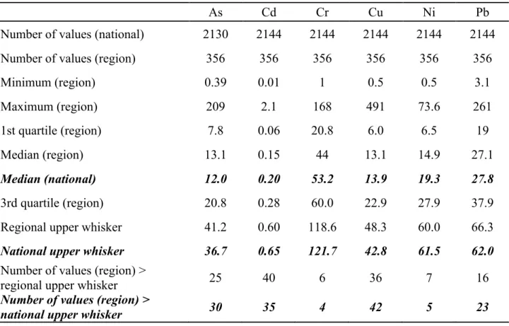
Table 1 presents the statistical characteristics of the concentrations of the trace elements 216
studied. The regional and national median values are close, which seems to show the 217
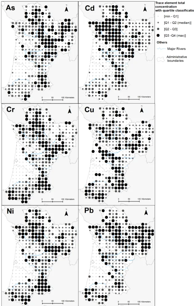
homogeneity of the concentrations in SWF compared to the whole of France. In more detail, 218
Figure 2 shows the maps of TE concentrations. The distribution of concentrations does not 219
appear to be regular. In particular, on the one hand, the Landes massif (around 15 % of the 220
soil samples) shows very low concentrations of the trace elements studied. On the other hand, 221
by defining the whiskers as anomaly thresholds, there are more sites with anomalous TE 222
concentrations (As, Cu, Pb) in the SWF according to the national threshold than according to 223
10
the regional threshold (Table 1). Therefore, there would be geogenic anomalies and/or 224
regional contaminations for As, Cu, and Pb while anomalies would be less substantial for Cd, 225
Cr and Ni. All of these observations highlight the interest of carrying out a more in-depth 226
spatial study in order in particular to locate these anomalies and identify their origin. In 227
addition, Table 2 presents the statistical characteristics of the soil variables considered in this 228
study. For all these variables, large amplitude of values is observed for the 356 soils sampled. 229
This is particularly the case for the concentrations of clay, pH, CaCO3, organic matter, Fe and
230
Al. Special attention was therefore granted to these variables, known to drive the TE 231
variability. 232
3.2 Multivariate analysis: first approach to the origin of the trace elements 233
In order to complete the previous observations by considering all the information points of the 234
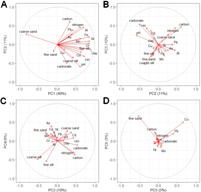
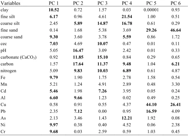
datasets, a multivariate analysis was carried out by PCA. Figure 3 presents, by decreasing 235
contributions, the 6 components (or dimensions) that explain 79% of the total variance. The 236
main contributions of the variables to the components are as follows (Table S1). The 237
concentrations of clay, coarse sand, Al, Fe, Cr, Ni, Cd and CEC for the principal component 1 238
(PC1); organic carbon, total nitrogen, pH and CaCO3 for principal component 2 (PC2); coarse
239
silt, CaCO3, CEC, pH and Cd for PC3; As, silt, carbon and nitrogen for PC4; fine sand, Pb
240
and Cu concentration for PC5; fine sand and Cu for PC6. The negative correlation between 241
coarse sands and TE concentrations suggests that soils with a high percentage of coarse sand 242
are rather poor in trace elements. This is confirmed by the lowest TE concentrations that are 243
located in the Landes forest, with mainly sandy soils of recent geological formation (<1 Ma), 244
and with an acidic pH which causes the solubilisation of the elements (Righi and Wilbert, 245
1984). In addition, sand has a lower specific surface, which does not promote the adsorption 246
of elements (Daskalakis and O’Connor, 1995; Schiff and Weisberg, 1999). 247
11 It can be also observed:
248
- In Figure 3A, the concentrations of Cr, Fe, Ni and the clay content correlate positively. 249
This suggests a rather geogenic origin of Cr and Ni. Indeed, the materials resulting from 250
the degradation of rocks rich in Cr and Ni are also rich in clays. Thus Cr, Ni and clays 251
would remain bound after the weathering of these rocks and transfer to the soil(Cheng et 252
al., 2011; Kierczak et al., 2007). This was observed in a previous study (ASPITET) on 253
trace elements in soils in France (Baize, 1997). 254
- In Figure 3B, Cd concentrations, CaCO3, pH and CEC also correlate positively. In the
255
study region, soils with high CaCO3 content, pH, and CEC are limestone soils. The
256
association between Cd and certain carbonate minerals could therefore explain this 257
correlation, as it was already observed in natural environments (Chada et al., 2005; Martin-258
Garin et al., 2002). This association is the result of the carbonate dissolution reaction, 259
where Cd2+ would replace Ca2+ to form CaCO3-CdCO3 or CdCO3 (Papadopoulos and
260
Rowell, 1988). The introduction of Cd into soils by amendments based on calcium 261
carbonates and phosphate fertilizers is also a possible source of Cd in soils (Senesil et al., 262
1999). 263
- In Figure 3C and 3D, no correlation could be noted for the concentrations of As, Cu and Pb 264
with the other variables in PCs that explain a low amount of the total variance. This 265
suggests rather a predominantly anthropogenic origin of these elements. 266
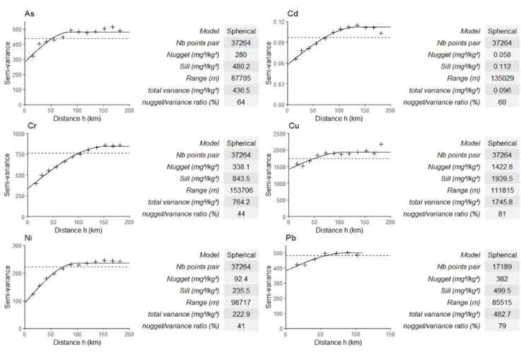
3.3 Spatial and geostatistical analysis: factors influencing spatial distribution 267
In order to bring a spatial dimension to the analysis of TE concentrations, their 268
semivariograms were calculated and are shown in Figure 4. These semivariograms were 269
obtained using equation (3) and are given with their associated parameters (especially nugget 270
effect, range and nugget/variance ratio; shown in the column to the right of each 271
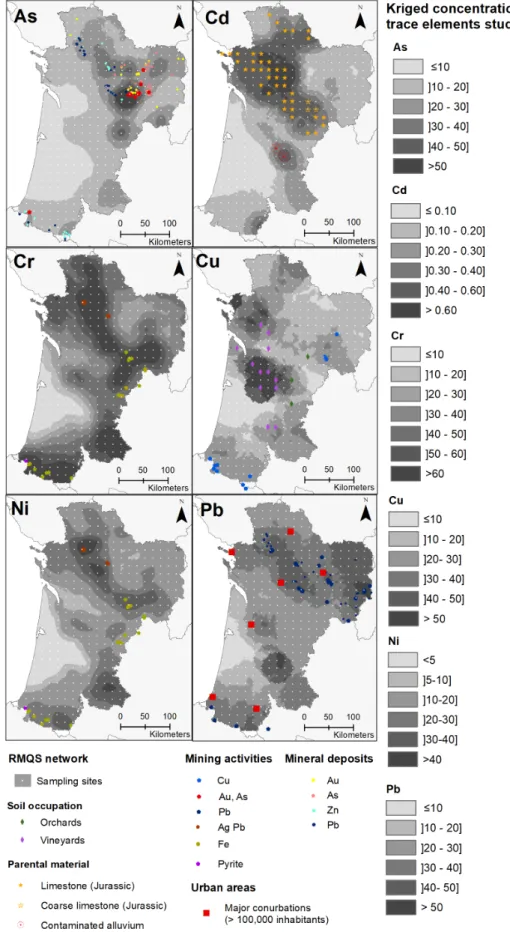
12
semivariogram). To complete, Figure 5 presents the thematic maps of the TE concentrations 272
predicted by ordinary kriging (using the parameters of the semivariograms of each trace 273
element). Geographical information on land use, mining activities, parent material and 274
mineral deposits are overlaid on concentration maps. Thus, all of the information obtained and 275
used can be viewed together. 276
All semivariograms (Figure 4) are bounded. This means that the spatial structures of the TE 277
concentrations are included in the regional study area. In other words, the concentrations of a 278
given trace element spatially depend on the range scale, which varies from 86 to 154 km 279
depending on the element considered. For all variograms, the nugget/variance ratios are 280
between 40 and 80 %. These values are partly induced by the size of the sampling grid 281
(16x16 km). This indicates that it was not possible to detect significant local variations. 282
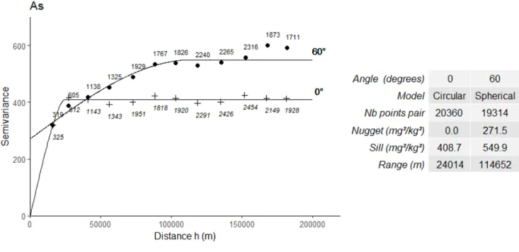
The directional analysis of the semivariograms revealed an anisotropy for As only, as 283
illustrated in Figure 6. The spatial structure of this element differs according to the direction 284
considered (as illustrated in the Figure S2 drawn in orthogonal directions north−south and 285
east−west). In particular, in the north−south direction (0°) the semivariogram is circular, 286
without nugget effect and with a very short range (24 km). In the northeast−east direction 287
(60°) the semivariogram is spherical, with a strong nugget effect and a range close to that of 288
the omnidirectional semivariogram (115 km). The direction of the directional semivariogram 289
of As (60°) points to the gold mining zones located to the north and northeast of the region. In 290
this area, the deposits consist of quartz veins containing native As and Au-As-S minerals 291
resulting from hydrothermal processes in granitic and metamorphic rocks (gneiss). 292
Consequently, As can be considered as a geochemical tracer of Au in this area (Bossy, 2010; 293
de Gramont and Braux, 1990). In addition, gold mining from the Gallic period until the end of 294
the 1960s led to the contamination of the Isle watershed by mining residues and therefore in 295
particular by As (Cauuet, 1991; Courtin-Nomade et al., 2002; Grosbois et al., 2007). 296
13
Cd does not exhibit a particularly high nugget/variance ratio (60 %) but has a greater range 297
compared to the majority of trace elements studied (> 135 km). This suggests a distribution of 298
Cd due to a single and extended source. In fact, and given that Cd is positively correlated with 299
pH and CEC, the presence of Cd would correspond to the presence of limestone substrates 300
(parent material and/or coarse fragments), therefore to a mainly geogenic origin. This is in 301
agreement with the work by Atteia et al. (1995) in the Swiss Jura and Baize et al. (1999) in 302
Bourgogne, where the Cd concentration was correlated with Jurassic age limestone. This 303
interpretation is also relevant insofar as such limestone soils of the same geological age are 304
present in the SWF, in particular in the departments of Dordogne and Charentes, i.e. in the 305
centre and northwest of the region, respectively (Figure 5). Very high Cd concentrations were 306
also found at two sites located on the alluvial deposits of the Garonne river (Figure 5). These 307
anomalies can be explained by the historical cadmium contamination of the Lot-Garonne 308
hydrological continuum that carries suspended matter directly from the Decazeville industrial 309
basin following the extraction and processing of ores rich in Zn and Cd or indirectly due to 310
the remobilization of sediments accumulated behind the dams of the Lot river (Audry et al., 311
2004; Coynel et al., 2009, 2007; Dabrin et al., 2009; Pougnet et al., 2019). 312
Cu has the highest nugget/variance ratio (81 %) and a large range (112 km), which can be 313
explained by the anthropogenic input of this element in the vineyards of the region (Figure 5). 314
Indeed, Cu has been used in viticulture in a mixture of copper sulphate and lime (Bordeaux 315
mixture) to fight against downy mildew (Peronospora viticola) since the end of the 19th 316
century (Ayres, 2004). This cultivation practice has led to diffuse soil contamination in 317
French wine-growing areas and in particular in Gironde, as mentioned in previous studies 318
(Baize et al., 2006; El Hadri et al., 2012). However, this contribution remains very 319
heterogeneous depending on the vine management technique chosen by the winegrowers as 320
well as the variability of the fungal pressure. 321
14
Cr and Ni have the lowest nugget/variance ratios (41 and 44% respectively). Less spatial 322
variability than for the other trace elements therefore appears for distances <16 km. This 323
suggests that the distribution of these two elements is mainly natural. This hypothesis would 324
be supported on the one hand by the fact that Cr and Ni are known to be not very mobile in 325
soils. On the other hand, these elements are usually found strongly adsorbed on the mineral 326
components of the soil such as calcite, illite and montmorillonite (Businelli et al., 2004; 327
Hickey and Kittrick, 1984; Mamindy-Pajany et al., 2013; Navarro-Pedreño et al., 2003). This 328
is relevant given the positive correlation with clays found above. The Cr and Ni 329
concentrations in SWF soils therefore appear to depend on the underlying bedrock, with high 330
concentrations being found in soils from Jurassic and Cretaceous rocks (Figure 5). This 331
dependence was already observed for the RMQS network at the national level (GIS Sol, 332
2011). Similar results were found by the FOREGS program on French soils (Salpeteur and 333
Maldan, 2011). If anthropogenic contaminations are possible, for example by spreading 334
sludge or due to industrial discharges, then they are probably very localised and therefore not 335
detected in the RMQS grid. 336
Pb has a high nugget/variance ratio (79%), with a lower range than the other elements (85 337
km). Its regional spatial distribution shows high concentrations in the north and northeast of 338
the region, with spots near large urban areas (Bordeaux, Bayonne, etc.) (Figure 5). 339
Concentrations in the northeast of the region are believed to be mainly of mining origin 340
(Courtin-Nomade et al., 2002; de Gramont and Braux, 1990). The spots close to large cities 341
are likely due to the density of traffic and the use of leaded gasoline until 2000 in France. The 342
work by Saby et al. (2006) led to a similar observation around the Paris urban area. Several Pb 343
spots are also found in forests and Pyrenean passes. They could come from hunting activities, 344
Pb shot being disseminated in soil samples (Mellor and McCartney, 1994; Tsuji and 345
Karagatzides, 1998). 346
15
3.4. Statistical approaches: representativeness and limits 347
The relatively high nugget/variance ratios obtained with semivariograms indicate that local 348
variations of TE concentrations cannot be detect by the 16x16 km grid. In other words, local 349
“hot spots” of TE concentrations may not be detected. Therefore, the issue of the 350
representativeness of the study on a regional scale could be raised. An analysis of the 351
representativeness of the different grid sizes (32x32, 16x16, 8x8 km) to design the RMQS 352
network was carried out (Arrouays et al., 2001). The analysis was based on the pair: soil type 353
– soil use pair. Results showed that with a 16x16 km grid, only 2.5% of the pairs are not 354
represented. In the SWF, the unrepresented part corresponds to small areas of vineyards and 355
orchards, which could have a significant input of TE. Targeted densification of the grid (e.g. 356
8x8 km) would help to better characterize these areas. However, this would also greatly 357
increase the number of sampling sites and consequently the implementation cost of the 358
network and the duration of the sampling. 359
In the present work we used upper whiskers as a first approach to detect anomalies in the TE 360
distribution. This simple approach, using descriptive statistics, has been widely used in 361
geochemical studies, including other studies based on the RMQS dataset (Redon et al., 2013; 362
Saby et al., 2009; Villanneau et al., 2008). However, it needs to be completed from other 363
approaches to discriminate between geogenic and anthropogenic anomalies. Saby et al. (2009) 364
determined the spatial patterns of TE over the whole of France with a spatially constrained 365
multivariate analysis method. The authors also identified the geogenic origin of Cd associated 366
with Jurassic limestone and the anthropogenic origin of Cu associated with the vineyard. At a 367
regional scale, Redon et al. (2013) combined the soil classification between calcareous and 368
non-calcareous soils, with several statistical methods (upper whiskers, enrichment factor, 369
PCA, linear regression) over the former Midi-Pyrénées region, adjacent to our study area. The 370
authors obtained similar results to ours, with Cu anomalies associated with the vineyard, but 371
16
found Cd and Pb contamination in grazing land suggesting sources from organic fertilization. 372
Finally, in the present work, we combined geostastistics and GIS that had the advantage of 373
producing intuitive maps with both TE concentrations anomalies and their associated sources. 374
4. Conclusion
375
The spatial distribution and variability of As, Cd, Cu, Cr, Ni, Pb for the south-western region 376
of France could be determined on the basis of the RMQS systematic sampling grid. The 377
regional median concentrations of these elements are close to the national values. However, 378
regional anomalous concentrations were highlighted by comparing with regional and national 379
whiskers taken as threshold values of anomaly and possible contamination. The origins of 380
these trace elements in SWF soils were identified combining cartographic and geostatistical 381
methods. Thus, As has a dual origin geogenic and anthropogenic, from gold deposit and 382
mining activities. Cu and Pb have anthropogenic origins, either linked to a main activity like 383
viticulture (Cu), or consecutive to several activities, mining, hunting and automobile traffic 384
(Pb). Cd, Cr and Ni are mainly of geogenic origin at the regional scale. In most cases, 385
contaminated areas are well demarcated. The Landes massif, with mostly sandy soils, contains 386
little content of trace elements. 387
The investigation approach used, combining systematic monitoring network and geostatistical 388
method, has thus shown its capability to detect contaminations in trace elements and to 389
identify their origins on a regional scale. This is possible despite a relatively large grid (16x16 390
km). This approach could therefore be transposable to countries with comparable surface 391
areas. Systematic soil monitoring networks have a dual interest: on the one hand, the data 392
acquired relating to soil quality can be used as a support element for national and regional 393
territorial decisions. This may concern environmental protection, agroecological transition or 394
food safety. On the other hand, these databases could be extended to other TE, not only those 395
17
monitored in the RMQS network but also to TE barely or not yet taken into account. 396
Emerging contaminations in the soil could then be identified. This would help to support 397
public decisions for the reduction and anticipation of pollution. This second point is 398
particularly important given the development of new technologies leading to an increasing use 399
of new elements (Alonso et al., 2012). These include the use of catalytic converters containing 400
platinoids (Pd, Pt, Rh), smartphones containing rare metals (such as Nd or Y) or MRI contrast 401
agents containing Gd (Lerat-Hardy et al., 2019; Schäfer et al., 1998). Finally, this type of 402
network could also enable changes in soil quality to be monitored by the early detection of 403
degradation that might be expected or not. A new campaign of soil sampling is ongoing for 404
the RMQS network. 405
Acknowledgments
406
This study was supported by a French Scientific Group of Interest on soils: the “GIS Sol”, 407
(involving the Ministry for an Ecological and Solidary Transition (MTES), the French 408
Ministry of Agriculture (MAA), the French Agency for Energy and Environment (ADEME), 409
the French Research Institute for Development (IRD), the French National Institute of 410
Geographic and Forest Information (IGN), the National Institute for Agronomic Research 411
(INRAE)) and Bordeaux Sciences Agro. Thanks are expressed to Claudy Jolivet, Céline Ratié 412
and Line Boulonne of unit INRAE US1106 InfoSol. We thank the three anonymous reviewers 413
for their comments that helped to improve this article. 414
18
References
416
AFNOR, 2003. NF X31-107.Qualité du sol. Détermination de la distribution granulométrique 417
des particules du sol. Méthode à la pipette. 418
AFNOR, 2001. NF ISO 14869-1.Qualité du sol. Mise en solution pour la détermination des 419
teneurs élémentaires totales. Partie 1: Mise en solution par l’acide fluorhydrique et l’acide 420
perchlorique. 421
AFNOR, 1999. NF X31-130. Qualité des sols. Méthodes chimiques. Détermination de la 422
capacité d’échange cationique (CEC) et des cations extractibles. 423
AFNOR, 1995a. NF ISO 10693. Qualité du sol. Détermination de la teneur en carbonate. 424
Méthode volumétrique. 425
AFNOR, 1995b. NF ISO 10694. Qualité du sol. Dosage du carbone organique et du carbone 426
total après combustion sèche (analyse élémentaire). 427
AFNOR, 1994a. NF ISO 11464. Qualité du sol. Prétraitement des échantillons pour analyses 428
physico-chimiques. 429
AFNOR, 1994b. ISO 10390. Qualité du sol. détermination du pH. 430
Alonso, E., Sherman, A.M., Wallington, T.J., Everson, M.P., Field, F.R., Roth, R., Kirchain, 431
R.E., 2012. Evaluating Rare Earth Element Availability: A Case with Revolutionary Demand 432
from Clean Technologies. Environ. Sci. Technol. 46, 3406–3414. 433
https://doi.org/10.1021/es203518d 434
Arrouays, D., Jolivet, C., Boulonne, L., Bodineau, G., Ratié, C., Saby, N., Grolleau, E., 2003. 435
Le réseau de mesures de la qualité des sols (RMQS) de France. Etude Gest. Sols 10, 241–250. 436
Arrouays, D., Thorette, J., Daroussin, J., 2001. Analyse de représentativité de différentes 437
configurations d’un réseau de sites de surveillance des sols. Etude Gest. Sols 8, 7–17. 438
Atteia, O., Dubois, J.-P., Webster, R., 1994. Geostatistical analysis of soil contamination in 439
the Swiss Jura. Environ. Pollut. 86, 315–327. https://doi.org/10.1016/0269-7491(94)90172-4 440
Atteia, O., Thélin, Ph., Pfeifer, H.R., Dubois, J.P., Hunziker, J.C., 1995. A search for the 441
origin of cadmium in the soil of the Swiss Jura. Geoderma 68, 149–172. 442
https://doi.org/10.1016/0016-7061(95)00037-O 443
Audry, S., Blanc, G., Schäfer, J., 2004. Cadmium transport in the Lot–Garonne River system 444
(France) – temporal variability and a model for flux estimation. Sci. Total Environ. 319, 197– 445
213. https://doi.org/10.1016/S0048-9697(03)00405-4 446
Ayres, P.G., 2004. Alexis Millardet: Frances forgotten mycologist. Mycologist 18, 23–26. 447
https://doi.org/10.1017/S0269915X04001090 448
Baize, D., 1997. Teneurs totales en éléments traces métalliques dans les sols (France): 449
Références et stratégies d’interprétation. Programme ASPITET, Un point sur. INRA, Paris. 450
Baize, D., Deslais, W., Gaiffe, M., 1999. Anomalies naturelles en cadmium dans les sols de 451
France. Etude Gest. Sols 2, 85–104. 452
Baize, D., Saby, N., Walter, C., 2006. Le cuivre extrait à l’EDTA dans les sols de France. 453
Etude Gest. Sols 13, 259–268. 454
19
Barcan, V., Kovnatsky, E., 1998. Soil Surface Geochemical Anomaly Around the Copper-455
Nickel Metallurgical Smelter. Water. Air. Soil Pollut. 103, 197–218. 456
https://doi.org/10.1023/A:1004930316648 457
Belon, E., Boisson, M., Deportes, I.Z., Eglin, T.K., Feix, I., Bispo, A.O., Galsomies, L., 458
Leblond, S., Guellier, C.R., 2012. An inventory of trace elements inputs to French agricultural 459
soils. Sci. Total Environ. 439, 87–95. https://doi.org/10.1016/j.scitotenv.2012.09.011 460
Bossy, A., 2010. Origines de l’arsenic dans les eaux, sols et sédiments du district aurifère de 461
St-Yrieix-la-Perche (Limousin, France)$: contribution du lessivage des phases porteuses 462
d’arsenic. Université de Limoges, Limoges. 463
BRGM, 2007. SIG Mines France [WWW Document]. URL 464
http://sigminesfrance.brgm.fr/index.asp (accessed 4.24.18). 465
BRGM, 2005. BD-CHARM$: Carte géologique de France à 1/50000 au format numérique 466
vecteur issue de la numérisation de la carte imprimée. 467
Businelli, D., Casciari, F., Gigliotti, G., 2004. Sorption mechanisms determining Ni(II) 468
retention by a calcareous soil. Soil Sci. 169, 355–362. 469
https://doi.org/10.1097/01.ss.0000128015.92396.56 470
Cauuet, B., 1991. L’exploitation de l’or en Limousin, des Gaulois aux Gallo-Romains. Ann. 471
Midi 103, 149–181. https://doi.org/10.3406/anami.1991.2292 472
Chada, V.G.R., Hausner, D.B., Strongin, D.R., Rouff, A.A., Reeder, R.J., 2005. Divalent Cd 473
and Pb uptake on calcite {101¯4} cleavage faces: An XPS and AFM study. J. Colloid 474
Interface Sci. 288, 350–360. https://doi.org/10.1016/j.jcis.2005.03.018 475
Chen, J., Wei, F., Zheng, C., Wu, Y., Adriano, D.C., 1991. Background concentrations of 476
elements in soils of China. Water Air Soil Pollut 57–58, 699–712. 477
https://doi.org/10.1007/BF00282934 478
Cheng, C.-H., Jien, S.-H., Iizuka, Y., Tsai, H., Chang, Y.-H., Hseu, Z.-Y., 2011. Pedogenic 479
Chromium and Nickel Partitioning in Serpentine Soils along a Toposequence. Soil Sci. Soc. 480
Am. J. 75, 659–668. https://doi.org/10.2136/sssaj2010.0007 481
Courtin-Nomade, A., Neel, C., Bril, H., Davranche, M., 2002. Trapping and mobilisation of 482
arsenic and lead in former mine tailings –Environmental conditions effects. Bull. Soc. Geol. 483
Fr. 173, 479–485. https://doi.org/10.2113/173.5.479 484
Coynel, A., Blanc, G., Marache, A., Schäfer, J., Dabrin, A., Maneux, E., Bossy, C., Masson, 485
M., Lavaux, G., 2009. Assessment of metal contamination in a small mining- and smelting-486
affected watershed: high resolution monitoring coupled with spatial analysis by GIS. J. 487
Environ. Monit. 11, 962–976. https://doi.org/10.1039/B818671E 488
Coynel, A., Schäfer, J., Dabrin, A., Girardot, N., Blanc, G., 2007. Groundwater contributions 489
to metal transport in a small river affected by mining and smelting waste. Water Res. 41, 490
3420–3428. https://doi.org/10.1016/j.watres.2007.04.019 491
Dabrin, A., Schäfer, J., Blanc, G., Strady, E., Masson, M., Bossy, C., Castelle, S., Girardot, 492
N., Coynel, A., 2009. Improving estuarine net flux estimates for dissolved cadmium export at 493
the annual timescale: Application to the Gironde Estuary. Estuar. Coast. Shelf Sci. 84, 429– 494
439. https://doi.org/10.1016/j.ecss.2009.07.006 495
Daskalakis, K.D., O’Connor, T.P., 1995. Normalization and Elemental Sediment 496
Contamination in the Coastal United States. Environ. Sci. Technol. 29, 470–477. 497
https://doi.org/10.1021/es00002a024 498
20
de Gramont, X., Braux, C., 1990. Synthèse Sud Limousin (No. R 31814 DEX-DAM-90), 499
Inventaire des ressources minières du territoire métropolitain. BRGM, Aubière. 500
El Hadri, H., Chéry, P., Jalabert, S., Lee, A., Potin-Gautier, M., Lespes, G., 2012. Assessment 501
of diffuse contamination of agricultural soil by copper in Aquitaine region by using French 502
national databases. Sci. Total Environ. 441, 239–247. 503
https://doi.org/10.1016/j.scitotenv.2012.09.070 504
Esri, 2012. ArcGIS Desktop. Environmental Systems Research Institute, Redlands. 505
Facchinelli, A., Sacchi, E., Mallen, L., 2001. Multivariate statistical and GIS-based approach 506
to identify heavy metal sources in soils. Environ. Pollut. 114, 313–324. 507
Farnham, I.M., Singh, A.K., Stetzenbach, K.J., Johannesson, K.H., 2002. Treatment of 508
nondetects in multivariate analysis of groundwater geochemistry data. Chemom. Intell. Lab. 509
Syst. 60, 265–281. https://doi.org/10.1016/S0169-7439(01)00201-5 510
GIS Sol, 2011. L’état des sols de France. Groupement d’intérêt scientifique sur les sols. 511
Grosbois, C., Courtin-Nomade, A., Martin, F., Bril, H., 2007. Transportation and evolution of 512
trace element bearing phases in stream sediments in a mining – Influenced basin (Upper Isle 513
River, France). Appl. Geochem. 22, 2362–2374. 514
https://doi.org/10.1016/j.apgeochem.2007.05.006 515
Hickey, M.G., Kittrick, J.A., 1984. Chemical Partitioning of Cadmium, Copper, Nickel and 516
Zinc in Soils and Sediments Containing High Levels of Heavy Metals. J. Environ. Qual. 13, 517
372–376. https://doi.org/10.2134/jeq1984.00472425001300030010x 518
Hou, D., O’Connor, D., Nathanail, P., Tian, L., Ma, Y., 2017. Integrated GIS and multivariate 519
statistical analysis for regional scale assessment of heavy metal soil contamination: A critical 520
review. Environ. Pollut. 231, 1188–1200. https://doi.org/10.1016/j.envpol.2017.07.021 521
IARC, 1993. Beryllium, cadmium, mercury, and exposures in the glass manufacturing 522
industry: views and expert opinions of an IARC Working Group on the Evaluation of 523
Carcinogenic Risks to Humans, which met in Lyon, 9 - 16 February 1993, IARC monographs 524
on the evaluation of carcinogenic risks to humans. Lyon. 525
[dataset] INRA, 2018. Base de Données Géographique des Sols de France à 1/1 000 000 526
version 3.2.8.0, 10/09/1998. Portail Data INRAE, V1. https://doi.org/10.15454/BPN57S 527
Jolivet, C., Boulonne, L., Ratié, C., 2006. Manuel du Réseau de mesures de la qualité des 528
sols, édition 2006. INRA, US 1106 InfoSol, Orléans. 529
Kierczak, J., Neel, C., Bril, H., Puziewicz, J., 2007. Effect of mineralogy and pedoclimatic 530
variations on Ni and Cr distribution in serpentine soils under temperate climate. Geoderma 531
142, 165–177. https://doi.org/10.1016/j.geoderma.2007.08.009 532
Lê, S., Josse, J., Husson, F., 2008. FactoMineR$: An R Package for Multivariate Analysis. J. 533
Stat. Softw. 25, 1–18. https://doi.org/10.18637/jss.v025.i01 534
Lerat-Hardy, A., Coynel, A., Dutruch, L., Pereto, C., Bossy, C., Gil-Diaz, T., Capdeville, M.-535
J., Blanc, G., Schäfer, J., 2019. Rare Earth Element fluxes over 15$years into a major 536
European Estuary (Garonne-Gironde, SW France): Hospital effluents as a source of 537
increasing gadolinium anomalies. Sci. Total Environ. 656, 409–420. 538
https://doi.org/10.1016/j.scitotenv.2018.11.343 539
Mamindy-Pajany, Y., Sayen, S., Guillon, E., 2013. Impact of sewage sludge spreading on 540
nickel mobility in a calcareous soil: adsorption–desorption through column experiments. 541
Environ. Sci. Pollut. Res. 20, 4414–4423. https://doi.org/10.1007/s11356-012-1357-3 542
21
Mandal, B., 2002. Arsenic round the world: a review. Talanta 58, 201–235. 543
https://doi.org/10.1016/S0039-9140(02)00268-0 544
Marchant, B.P., Saby, N.P.A., Arrouays, D., 2017. A survey of topsoil arsenic and mercury 545
concentrations across France. Chemosphere 181, 635–644. 546
https://doi.org/10.1016/j.chemosphere.2017.04.106 547
Marchant, B.P., Saby, N.P.A., Lark, R.M., Bellamy, P.H., Jolivet, C.C., Arrouays, D., 2010. 548
Robust analysis of soil properties at the national scale: cadmium content of French soils. Eur. 549
J. Soil Sci. 61, 144–152. https://doi.org/10.1111/j.1365-2389.2009.01212.x 550
Martin-Garin, A., Gaudet, J.P., Charlet, L., Vitart, X., 2002. A dynamic study of the sorption 551
and the transport processes of cadmium in calcareous sandy soils. Waste Manag. 22, 201– 552
207. https://doi.org/10.1016/S0956-053X(01)00070-8 553
McGrath, S.P., Loveland, P.J., 1992. The soil geochemical atlas of England and Wales. 554
Blackie Academic & Professional, Glasgow. 555
McLaughlin, M.J., Parker, D.R., Clarke, J.M., 1999. Metals and micronutrients – food safety 556
issues. Field Crops Res. 60, 143–163. https://doi.org/10.1016/S0378-4290(98)00137-3 557
Mellor, A., McCartney, C., 1994. The effects of lead shot deposition on soils and crops at a 558
clay pigeon shooting site in northern England. Soil Use Manag. 10, 124–129. 559
https://doi.org/10.1111/j.1475-2743.1994.tb00472.x 560
Morvan, X., Saby, N.P.A., Arrouays, D., Le Bas, C., Jones, R.J.A., Verheijen, F.G.A., 561
Bellamy, P.H., Stephens, M., Kibblewhite, M.G., 2008. Soil monitoring in Europe: A review 562
of existing systems and requirements for harmonisation. Sci. Total Environ. 391, 1–12. 563
https://doi.org/10.1016/j.scitotenv.2007.10.046 564
Navarro-Pedreño, J., Almendro-Candel, M.B., Jordan-Vidal, M.M., Mataix-Solera, J., Garcia-565
Sanchez, E., 2003. Mobility of cadmium, chromium, and nickel through the profile of a 566
calcisol treated with sewage sludge in the southeast of Spain. Environ. Geol. 44, 545–553. 567
https://doi.org/10.1007/s00254-003-0790-5 568
Orgiazzi, A., Ballabio, C., Panagos, P., Jones, A., Fernández Ugalde, O., 2018. LUCAS Soil, 569
the largest expandable soil dataset for Europe: a review. European Journal of Soil Science 69, 570
140–153. https://doi.org/10.1111/ejss.12499 571
Papadopoulos, P., Rowell, D.L., 1988. The reactions of cadmium with calcium carbonate 572
surfaces. J. Soil Sci. 39, 23–36. https://doi.org/10.1111/j.1365-2389.1988.tb01191.x 573
Pebesma, E.J., 2004. Multivariable geostatistics in S: the gstat package. Comput. Geosci. 30, 574
683–691. https://doi.org/10.1016/j.cageo.2004.03.012 575
Pougnet, F., Blanc, G., Mulamba-Guilhemat, E., Coynel, A., Gil-Diaz, T., Bossy, C., Strady, 576
E., Schäfer, J., 2019. Nouveau modèle analytique pour une meilleure estimation des flux nets 577
annuels en métaux dissous. Cas du cadmium dans l’estuaire de la Gironde. Hydroécologie 578
Appliquée. https://doi.org/10.1051/hydro/2019002 579
R Core Team, 2019. R: A language and environment for statistical computing. R Foundation 580
for Statistical Computing, Vienna, Austria. 581
Ranjard, L., Nowak, V., Echairi, A., Faloya, V., Chaussod, R., 2008. The dynamics of soil 582
bacterial community structure in response to yearly repeated agricultural copper treatments. 583
Res. Microbiol. 159, 251–254. https://doi.org/10.1016/j.resmic.2008.02.004 584
22
Redon, P.-O., Bur, T., Guiresse, M., Probst, J.-L., Toiser, A., Revel, J.-C., Jolivet, C., Probst, 585
A., 2013. Modelling trace metal background to evaluate anthropogenic contamination in 586
arable soils of south-western France. Geoderma 206, 112–122. 587
https://doi.org/10.1016/j.geoderma.2013.04.023 588
Reimann, C., Filzmoser, P., Garrett, R.G., 2005. Background and threshold: critical 589
comparison of methods of determination. Sci. Total Environ. 346, 1–16. 590
https://doi.org/10.1016/j.scitotenv.2004.11.023 591
Righi, D., Wilbert, J., 1984. Les sols sableux podzolisés des Landes de Gascogne (France): 592
répartition et caractères principaux. Science du sol, 253–264. 593
Rooney, C.P., Zhao, F.-J., McGrath, S.P., 2007. Phytotoxicity of nickel in a range of 594
European soils: Influence of soil properties, Ni solubility and speciation. Environ. Pollut. 145, 595
596–605. https://doi.org/10.1016/j.envpol.2006.04.008 596
Saby, N., Arrouays, D., Boulonne, L., Jolivet, C., Pochot, A., 2006. Geostatistical assessment 597
of Pb in soil around Paris, France. Sci. Total Environ. 367, 212–221. 598
https://doi.org/10.1016/j.scitotenv.2005.11.028
599
[dataset] Saby, N., Bertouy, B., Boulonne, L., Bispo, A., Ratié, C., Jolivet, C., 2019. 600
Statistiques sommaires issues du RMQS sur les données agronomiques et en éléments traces 601
des sols français de 0 à 50 cm. Portail Data INRAE, V5. https://doi.org/10.15454/BNCXYB 602
Saby, N., Marchant, B.P., Lark, R.M., Jolivet, C.C., Arrouays, D., 2011. Robust geostatistical 603
prediction of trace elements across France. Geoderma 162, 303–311. 604
https://doi.org/10.1016/j.geoderma.2011.03.001 605
Saby, N., Thioulouse, J., Jolivet, C.C., Ratié, C., Boulonne, L., Bispo, A., Arrouays, D., 2009. 606
Multivariate analysis of the spatial patterns of 8 trace elements using the French soil 607
monitoring network data. Sci. Total Environ. 407, 5644–5652. 608
https://doi.org/10.1016/j.scitotenv.2009.07.002 609
Salminen, R., 2005. Geochemical atlas of Europe Pt. 1. Background information, 610
methodology and maps. Geological Survey of Finland, Espoo. 611
Salpeteur, I., Maldan, F., 2011. French geochemical baseline data for trace elements in top- 612
and bottom-soils and overbanks of the shield areas and sediment covers: A low density survey 613
in the FOREGS Geochemical Atlas of Europe (II). Environ. Risques Santé 299–315. 614
https://doi.org/10.1684/ers.2011.0479 615
Schäfer, J., Hannker, D., Eckhardt, J.-D., Stüben, D., 1998. Uptake of traffic-related heavy 616
metals and platinum group elements (PGE) by plants. Sci. Total Environ. 215, 59–67. 617
https://doi.org/10.1016/S0048-9697(98)00115-6 618
Schiff, K.C., Weisberg, S.B., 1999. Iron as a reference element for determining trace metal 619
enrichment in Southern California coastal shelf sediments. Mar. Environ. Res. 48, 161–176. 620
https://doi.org/10.1016/S0141-1136(99)00033-1 621
Senesil, G.S., Baldassarre, G., Senesi, N., Radina, B., 1999. Trace element inputs into soils by 622
anthropogenic activities and implications for human health. Chemosphere, Matter and Energy 623
Fluxes in the Anthropocentric Environment 39, 343–377. https://doi.org/10.1016/S0045-624
6535(99)00115-0 625
Shacklette, H.T., Boerngen, J.G., 1984. Element concentrations in soils and other surficial 626
materials of the conterminous United States. USGS Professional Paper 1270. 627
23
Tsuji, L.J.S., Karagatzides, J.D., 1998. Spent lead shot in the western James Bay region of 628
northern Ontario, Canada: Soil and plant chemistry of a heavily hunted wetland. Wetlands 18, 629
266–271. https://doi.org/10.1007/BF03161662 630
Tukey, J.W., 1977. Exploratory data analysis, Addison-Wesley series in behavioral science$: 631
quantitative methods. Addison-Wesley, Reading. 632
Villanneau, E., Perry-Giraud, C., Saby, N., Jolivet, C., Marot, F., Maton, D., Floch-Barneaud, 633
A., Antoni, V., Arrouays, D., 2008. Détection de valeurs anomaliques d’éléments traces 634
métalliques dans les sols à l’aide du Réseau de Mesure de la Qualité des Sols. Etude et 635
Gestion des sols 15, 183–200. 636
Webster, R., Oliver, M.A., 1993. How large a sample is needed to estimate the regional 637
variogram adequately?, in: Soares, A. (Ed.), Geostatistics Tróia ’92: Volume 1, Quantitative 638
Geology and Geostatistics. Springer Netherlands, Dordrecht, pp. 155–166. 639
https://doi.org/10.1007/978-94-011-1739-5_14 640
Zehetner, F., Rosenfellner, U., Mentler, A., Gerzabek, M.H., 2009. Distribution of Road Salt 641
Residues, Heavy Metals and Polycyclic Aromatic Hydrocarbons across a Highway-Forest 642
Interface. Water. Air. Soil Pollut. 198, 125–132. https://doi.org/10.1007/s11270-008-9831-8 643
24 644
Figure 1: A) Map describing the administrative divisions of the study area and major natural areas. B) Map 645
of dominant soils from the Soil Geographical Data Base of France (BDGSF) at scale 1:1000000 (INRA, 646
2018). C) Map of the dominant parent material from the BDGSF. 647
25
Figure 2: Point distribution of As, Cd, Cr, Cu, Ni and Pb concentrations with classification by quartile in 649
the topsoil of southwestern France. 650
26
Figure 3: Variable factor maps of the principal components analysis. On each axis, in bracket, 651
the percentage of variance explained by the principal components (PC). A) PC 1 and PC 2; B) 652
PC 2 and PC 3; C) PC 3 and 4 D) PC 5 and PC 6. 653
27 654
655
Figure 4: Omnidirectional semivariograms, experimental (cross), and fitted with spherical model 656
(black line). Dashed line corresponds to the total variance. Pb experimental semivariogram is cut 657
from 100,000 meters because the semivariance decreases sharply after this distance. The data at the 658
top right of each graph describe the modeled semivariograms. For each semivariogram the number 659
(nb) of points pair is superior to 50 (Webster and Oliver, 1993). 660
28 661
Figure 5: Maps with kriged concentrations of studied trace elements, and geographic information 662
describing soil occupation, geology, mineral deposits and mining activities over the SWF. Soil 663
occupation and geological data are shown on maps over sampling sites and originate from site 664
description and geological maps, respectively (BRGM, 2005). Mineral deposits and mining activities 665
data are shown on the maps at their exact location (BRGM, 2007). 666
29 668
669
Figure 6: Directional semivariograms of As. Crosses represent 0° semivariance data, dots represent 670
60°semivariance data. For each semivariance value, the number of point pair is shown. The solid lines 671
represent the modeled semivariograms, with their descriptive parameters to the right of the figure. 672
30
Table 1: Descriptive statistics of As, Cd, Cr, Cu, Ni and Pb total concentrations in soils (in mg/kg) and 674
assessment of anomalous values at regional and national scales (Saby et al., 2019). Regional values 675
are included in the national dataset. 676
!! As Cd Cr Cu Ni Pb
Number of values (national) 2130 2144 2144 2144 2144 2144
Number of values (region) 356 356 356 356 356 356
Minimum (region) 0.39 0.01 1 0.5 0.5 3.1 Maximum (region) 209 2.1 168 491 73.6 261 1st quartile (region) 7.8 0.06 20.8 6.0 6.5 19 Median (region) 13.1 0.15 44 13.1 14.9 27.1 Median (national) 12.0 0.20 53.2 13.9 19.3 27.8 3rd quartile (region) 20.8 0.28 60.0 22.9 27.9 37.9
Regional upper whisker 41.2 0.60 118.6 48.3 60.0 66.3
National upper whisker 36.7 0.65 121.7 42.8 61.5 62.0
Number of values (region) >
regional upper whisker 25 40 6 36 7 16
Number of values (region) >
31
Table 2: Descriptive statistics of granulometry, pH, CaCO3, carbon, nitrogen, total Al, Fe and
677
Mn of the 356 soil samples. 678
679
Variable unit Min quartile 1st Median quartile 3rd Max
Clay % 0.2 12.58 19.75 32.3 65.2 Fine silt % 0.1 12.43 19.25 26.53 45.3 Coarse silt % 0.1 6.7 11.05 16.6 38.6 Fine sand % 0.5 8.28 12 16.13 59.8 Coarse sand % 0.6 10.83 23.85 49.15 97 CaCO3 g/kg 0.5 0.5 0.5 2.05 706 pH 4 4.9 5.8 7.4 8.4 CEC cmolc/k g 0.25 3.84 6.61 17.33 50.6 Organic carbon % 0.059 1.22 1.73 2.68 13.4 Total nitrogen ‰ 0.03 0.94 1.50 2.3 9.79 Al % 0.12 2.52 4.44 6.66 10.2 Fe % 0.03 1.08 2.17 3.14 7.66 Mn mg/kg 5 195.8 485.5 738.5 4870 680 681
32
Supplementary materials:
682
683 684
Figure S1: A) Location of RMQS sampling sites in the survey area. B) Illustration of the 685
sampling process applied on the RMQS sites. Modified from Jolivet et al. (2006). During the 686
first campaign. samples were taken from the subsquares numbered 1. 687
688 689
690
Figure S2: Experimental bidirectional variograms shown as a raster with a 16.000 m wide tile. 691
The X-axis represents west-east direction and the Y-axis represents north-south direction. 692
33
Table S1: Contribution of variables to each dimension of the PCA (%). The highest contributions 693 (>5.3%) are in bold. 694 Variables PC 1 PC 2 PC 3 PC 4 PC 5 PC 6 clay 10.52 0.72 1.57 0.03 0.00001 0.93 fine silt 6.17 0.96 4.61 21.54 1.00 0.51 coarse silt 2.45 5.89 14.87 16.78 0.61 0.29 fine sand 0.14 1.68 5.38 3.69 29.26 46.64 coarse sand 9.30 3.60 3.78 5.59 0.86 1.72 cec 7.03 4.69 10.07 0.47 0.01 0.11 pH 5.05 16.47 3.09 2.42 0.01 0.33 carbonate (CaCO3) 0.92 11.85 15.10 0.84 0.29 0.65 carbon 1.57 17.64 11.37 9.48 1.04 6.21 nitrogen 5.09 9.83 10.03 6.89 0.61 4.87 Fe 9.79 1.90 1.75 2.78 1.58 0.54 Mn 5.21 1.24 4.91 2.89 0.48 3.30 Cd 5.46 1.98 7.26 3.95 0.05 0.24 Al 6.60 9.66 1.23 0.02 0.49 0.25 Cu 0.58 0.91 0.55 4.37 44.10 26.41 Pb 2.35 7.12 0.00 0.95 16.59 4.09 As 2.13 3.46 1.43 12.21 1.92 0.08 Ni 9.97 0.38 0.40 4.52 0.06 2.38 Cr 9.68 0.03 2.59 0.59 1.03 0.45 695