HAL Id: insu-02123764
https://hal-insu.archives-ouvertes.fr/insu-02123764
Submitted on 9 May 2019HAL is a multi-disciplinary open access archive for the deposit and dissemination of sci-entific research documents, whether they are pub-lished or not. The documents may come from teaching and research institutions in France or abroad, or from public or private research centers.
L’archive ouverte pluridisciplinaire HAL, est destinée au dépôt et à la diffusion de documents scientifiques de niveau recherche, publiés ou non, émanant des établissements d’enseignement et de recherche français ou étrangers, des laboratoires publics ou privés.
reduced-complexity model
Thomas Croissant, Philippe Steer, Dimitri Lague, Philippe Davy, Louise
Jeandet, Robert Hilton
To cite this version:
Thomas Croissant, Philippe Steer, Dimitri Lague, Philippe Davy, Louise Jeandet, et al.. Seismic cycles, earthquakes, landslides and sediment fluxes: Linking tectonics to surface processes using a reduced-complexity model. Geomorphology, Elsevier, 2019, 339, pp.87-103. �10.1016/j.geomorph.2019.04.017�. �insu-02123764�
Seismic cycles, earthquakes, landslides and sediment fluxes:
Linking tectonics to surface processes using a reduced-complexity
model
Thomas Croissant, Philippe Steer, Dimitri Lague, Philippe Davy,
Louise Jeandet, Robert G. Hilton
PII:
S0169-555X(19)30166-7
DOI:
https://doi.org/10.1016/j.geomorph.2019.04.017
Reference:
GEOMOR 6745
To appear in:
Geomorphology
Received date:
27 December 2018
Revised date:
15 April 2019
Accepted date:
17 April 2019
Please cite this article as: T. Croissant, P. Steer, D. Lague, et al., Seismic cycles,
earthquakes, landslides and sediment fluxes: Linking tectonics to surface processes using
a
reduced-complexity
model,
Geomorphology,
https://doi.org/10.1016/
j.geomorph.2019.04.017
This is a PDF file of an unedited manuscript that has been accepted for publication. As
a service to our customers we are providing this early version of the manuscript. The
manuscript will undergo copyediting, typesetting, and review of the resulting proof before
it is published in its final form. Please note that during the production process errors may
be discovered which could affect the content, and all legal disclaimers that apply to the
journal pertain.
ACCEPTED MANUSCRIPT
1
Seismic cycles, earthquakes, landslides and sediment fluxes: linking
tectonics to surface processes using a reduced-complexity model
Thomas Croissant1,2*, Philippe Steer1,Dimitri Lague1, Philippe Davy1, Louise Jeandet1 and Robert G. Hilton2
1
Géosciences Rennes, OSUR, CNRS, Université de Rennes 1, Campus de Beaulieu, Rennes
2
Department of Geography, Durham University, Durham, DH1 3LE, UK
*
Corresponding author: T. Croissant; [email protected]
Abstract
In tectonically active mountain ranges, landslides triggered by earthquakes mobilise large volumes of sediment that affect river dynamics. This sediment delivery can cause downstream changes in river geometry and transport capacity that affect the river efficiency to export this sediment out of the epicentre area. The subsequent propagation of landslide deposits in the fluvial network has implications for the management of hazards downstream and for the longer-term evolution of topography over multiple seismic cycles. A full understanding of the processes and time scales associated with the removal of landslide sediment by rivers following earthquakes however, is still lacking. Here, we propose a nested numerical approach to investigate the processes controlling the post-seismic sediment evacuation at the mountain range scale, informed by results from a reach scale model. First, we explore the river morphodynamic response to a landslide cascade at the reach-scale using a 2D modelling approach. The results are then used to describe empirically the evacuation of a landslide volume which avoids using a computationally extensive model in catchments which may have thousands of co-seismic landslides. Second, we propose a reduced-complexity model to quantify evacuation times of earthquake-triggered landslide clusters at the scale of a mountain range, examining the hypothetical case of a Mw 7.9 earthquake and its aftershocks occurring on the Alpine Fault, New
Zealand. Our approach combines an empirical description of co-seismic landslide clusters with the sediment export processes involved during the post-seismic phase. Our results show that the inter-seismic capacity of the mountain range to evacuate co-seismic sediment is critical to assess the sediment budget of large earthquakes, over one to several seismic cycles. We show that
ACCEPTED MANUSCRIPT
2
sediment evacuation is controlled by two timescales, 1. the transfer time of material from hillslopes to channels and 2. the evacuation time of the landslide deposits once it has reached the fluvial network. In turn, post-seismic sediment evacuation can either be connectivity-limited, when sediment delivery along hillslopes is the main limiting process, or transport-limited, when the transport by rivers is the limiting process. Despite high values of runoff, we suggest that the Southern Alps of New Zealand are likely to be in connectivity-limited conditions, for connection velocities less than 10 m.yr-1. Connection velocities greater than2 m.yr-1 are sufficient to allow most of co-seismic sediments to be mobilised and potentially exported out of the range within less that one seismic cycle. Because of the poorly-constrained rate of sediment transfer along hillslopes, our results potentially raise the issue of co-seismic sediment accumulation within mountain ranges over several seismic cycles and of the imbalance between tectonic inputs and sediment export. We, therefore, call for renewed observational efforts to better describe and quantify the physical processes responsible for the redistribution and mobilization of sediment from landslide scars and deposits.
Key words: landslide, earthquake, river morphodynamics, landscape evolution.
1. Introduction
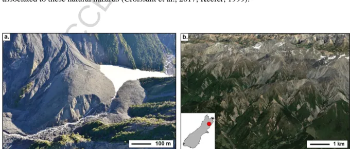
Earthquakes impact the landscapes of active mountain ranges by mobilizing large volumes of sediment through widespread landsliding (Malamud et al., 2004b; Ouimet, 2011) (Fig. 1). These clusters of landslides can deliver sediment to the fluvial network and affect its dynamics over timescales lasting from decades to centuries (Croissant et al., 2017; Hovius et al., 2011; Wang et al., 2015; Wang et al., 2017; Yanites et al., 2010). Whereas numerous studies have focused on the co-seismic response of hillslopes to large earthquakes (e.g. Gallen et al., 2015; Keefer, 1984, 1999; Malamud et al., 2004a; Marc et al., 2016; Meunier et al., 2007, 2008), comparatively few have investigated the post-seismic evolution of landscapes and sediment transport (e.g. Yanites et al., 2010; Hovius et al., 2011; Croissant et al., 2017). This probably results from extensive datasets constraining co-seismic landsliding and sediment production (Keefer, 1999; Larsen et al., 2010; Li et al., 2014;
ACCEPTED MANUSCRIPT
3
Malamud et al., 2004a; Marc et al., 2016; Tanyaş et al., 2017, 2018), while it is more challenging to obtain measurements of pre- and post-seismic sediment fluxes and topographic changes over tens of years. Most of the observations relate to suspended sediment concentration data (Dadson et al., 2004; Hovius et al., 2011; Wang et al., 2015; Wang et al., 2017) completed with analytical and numerical models of bedload evacuation (Croissant et al., 2017; Yanites et al., 2010).
Investigating how fluvial systems digest these abrupt and large sediment pulses is critical for sediment transfers (Benda & Dunne, 1997), bedrock incision patterns in landslide-dominated mountain ranges (Lague, 2010; Yanites et al., 2011), hydro-sedimentary hazards in alluvial fans (Croissant et al., 2017; Robinson & Davies, 2013) and even to quantify the feedbacks of surface processes on fault stress loading (Steer et al., 2014). They are also relevant to geochemical fluxes from mountain belts, particularly those which relate to soil erosion and organic carbon transfer (Wang et al., 2016) and inorganic carbon via silicate and carbonate weathering which can take place in landslide deposits (Emberson et al., 2016a; Jin et al., 2016). Over short-times scales (i.e. < 1000 years), the downstream propagation of sediment pulses have been studied principally at the reach scale using flume experiments and 1D numerical modelling (Cui et al., 2003; Cui & Parker, 2005; Lisle et al., 2001; Sklar et al., 2009; Sutherland et al., 2002). These studies have focused, however, primarily on the end-member case of how a low amplitude sediment supply compares to the transport capacity of the river. Croissant et al, [2017] proposed a 2D morphodynamic approach that examines high-amplitude sediment supplies compared to the transport capacity of the river. In the latter case, the role of dynamic river narrowing in accelerating the removal of landslide-driven sediments is critical. Despite these recent efforts, a full understanding of post-seismic sediment fluxes at the mountain range scale is still lacking.
Post-seismic sediment export is controlled by the sediment supply delivered by the landslide and by the transport capacity of the river receiving the deposit. The quantity of sediment transported by the river is, therefore, likely to be strongly dependent on the degree of connectivity of sources (landslides) to the fluvial network at the initial stage and through time (Hovius et al., 2000). Several studies have provided a quantification of the initial percentage of earthquake-triggered landslides that connect to the drainage network, ranging from 8% to nearly full connectivity (Dadson et al., 2004; Li
ACCEPTED MANUSCRIPT
4
et al., 2016; West et al., 2011). Work on the temporal evolution of connectivity through time, however, remains an open question (Zhang et al., 2016). Landslides connected directly to the river network can inject an almost instantaneous sediment load to the river. Landslides deposits that remain on the hillslope are likely to deliver the sediment in a more progressive manner, depending also on post-seismic storms (Fan et al., 2018). Once sediments mobilized by landslides reach the river channel, their export time is expected to depend mostly on the river geometry, discharge and on sediment grain size (Croissant et al., 2017). Whereas the evacuation of one landslide has already received attention, no work has been dedicated to the evacuation of seismically-triggered clusters of landslides.
The distributions of landslides can statistically inform on the dynamics of connectivity and subsequent export by river transport. For instance, landslides older than several seismic cycles and persisting in the landscapes have been argued to indicate a low efficiency of sediment export (Korup, 2005b). Such inference, however, cannot be made solely based on individual and old landslides, which represent outliers of the total cluster of landslides triggered by earthquakes or rainfall. Understanding the triggering and export of landslide clusters over several seismic cycles is required to assess the topographic budget of large earthquakes (Parker et al., 2011), the role of aftershocks relatively to mainshocks, sediment fluxes at the range scale (Hovius et al., 1997), the geochemical signature of these extreme events (Frith et al., 2018; Wang et al., 2016), or the impact and risks associated to these natural hazards (Croissant et al., 2017; Keefer, 1999).
Figure 1 | Illustration of the geomorphic impact of landslides at different spatial scales a. Aerial image of the Hapuku river landslide (taken the 5th Dec. 2016) triggered by the 2016 Kaikoura
ACCEPTED MANUSCRIPT
5
earthquake, New Zealand (photo credit: D. Townsend, GNS) b. Satellite image of the area affected by the Kaikoura earthquake that triggered thousands of landslides (source: Google Earth, imagery date 22/11/2016).
In this study, we develop a nested numerical approach which acts to: 1. simulate earthquakes over several seismic cycles, 2. trigger landslides across catchments, 3. assign the dynamic connectivity to the fluvial network and 4. determine the subsequent sediment transport. Our approach is deliberatively simplified to examine the challenges that emerge when investigating post-seismic sediment evacuation. The nested model integrates sediment export times defined at the reach scale, using the Eros river morphodynamic model (e.g. Davy et al., 2017; Croissant et al., 2017), in a statistical model that generates earthquakes and landslides at the mountain range scale, refered to as Quakos. The paper is divided in three sections. First, at the reach-scale, we investigate the impact of one or a series of landslides on the morphodynamic response of a river, the efficiency of sediment export and the persistence of downstream deposits. This allows us to develop a semi-analytical model of landslide export. Second, we focus on embedding the reach-scale model outcomes into the catchment-scale model. We define a reduced-complexity model that accounts for the different processes driving the sediment export of landslide debris that can be applied to clusters of landslides triggered by earthquakes. We apply this model to the case of a hypothetical Mw 7.9 earthquake
occurring in the Southern Alps of New Zealand. Third, we investigate the morphological impact of a series of earthquakes on landscape dynamics at the mountain range scale. We focus specifically on the roles of the dynamic connectivity of landslide deposits and runoff that modulate river transport capacity. Our results illustrate how the model parametrization impacts the number and volume of triggered landslides, the time persistence, the sediment fluxes leaving the mountain range and the evolution of landslide-size distributions. This leads us to highlight research needs and critical steps required to better understand and predict the impact of large earthquakes on landscape evolution and sediment fluxes.
ACCEPTED MANUSCRIPT
6
In this section, we explore the fine-scale dynamics of sediment export of a river that is impacted by a cascade of landslides. We first describe the 2D morphodynamic model Eros that we use to quantify the evacuation of individual landslides at the reach scale (Croissant et al., 2017; Davy et al., 2017). Following Croissant et al. (2017), we present the mechanisms controlling the downstream propagation of a single landslide deposited in a bedrock channel. We then explore the impact of a cascade of landslides on sediment export by introducing several landslides along the same river channel. In addition to revealing the morphodynamic evolution of the landslide deposits, the results from this section will be used in the Quakos study to tackle evacuation of landslide clusters over large areas.
2.1 Model description
This study is placed in the context of a bedrock river experiencing a high amplitude sediment forcing that causes perturbations of the river geometry including its width and slope. Therefore, an accurate quantification of landslide removal at the reach scale requires a model that contains the physical processes allowing for the feedbacks between river erosion, transport capacity, flow, geometry and sediment supply. Here, we use Eros (Davy et al., 2017), a particle-based model that is well-suited to simulate the evolution of a river subjected to large sediment supplies (Croissant et al, 2017a, b). The particles referred as “precipitons” are elementary volumes of water that move on the top of the topography and interact with it along the downstream path by entraining, transporting or depositing sediment. This model is composed of:
- A hydrodynamic model that predicts water depth and flow velocity patterns on high resolution topographies (Davy et al, 2017). This model resolves the 2D shallow-water equations under the stationary assumption without inertia.
- A vertical and horizontal sediment transport and deposition model that is coupled with the hydrodynamic model. In the following, we only briefly describe the constitutive equations of sediment entrainment, transport and deposition, as a more detailed description can be found Davy et al., [2017]. The rate of sediment entrainment, 𝑒̇, is defined by the bedload transport law of Meyer-Peter and Muller [1948]:
ACCEPTED MANUSCRIPT
7
𝑒̇ = 𝐸(𝜏 − 𝜏𝑐)1.5 (1)
with 𝐸 a constant, 𝜏, the shear stress and 𝜏𝑐 the critical shear stress. The rate of sediment deposition 𝑑̇
is a function of the sediment specific discharge 𝑞𝑠 and transport length, 𝜉 (Davy & Lague, 2009):
𝑑̇ =𝑞𝑠
𝜉 (2)
In the morphodynamic simulations, 𝜉 is set to 2 m to insure a bedload transport regime where the flow is close to at-capacity conditions in non-supply-limited cases. The model also includes horizontal sediment dynamics. The lateral erosion of neighboring cells is described by:
𝑒̇𝑙𝑎𝑡= 𝑘𝑒𝑆𝑦𝑒̇ (3)
with 𝑘𝑒 a dimensionless coefficient (here set at 0.05 as in Croissant et al [2017]) and 𝑆𝑦 the slope in
the transverse direction. The lateral sediment deposition 𝑞𝑠𝑙 is defined as:
𝑞𝑠𝑙 = 𝑘𝑑𝑞𝑠𝑆𝑦 (4)
with 𝑘𝑑 a constant (here set to 0.5). The choice of parameter values emerges from different
calibrations studies (e.g. Davy et al, 2017, Croissant et al, 2017).
The model allows for self-formed channels to emerge and for instabilities, such as bars and braiding, to develop (i.e. the river flow to converge in a self-formed width) when the local sediment flux is non-linearly correlated with the river discharge. In Eros simulations presenting a simple tilted bed as initial topography and no sediment input, Eros shows that the river width that emerges scales with discharge at a power 0.5 which is similar to that measured on natural cases and in flume experiments (e.g. Métivier et al., 2017).
2.2 Initial topography and boundary conditions
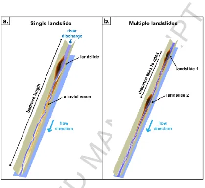
The model setup is similar to the one used in Croissant et al., [2017]. The initial topography is a 3 km long bedrock channel. Its transport capacity is set by its width and slope (Fig. 2a). The water enters through the upstream boundary condition at a constant effective discharge. The landslide deposit is introduced near the upstream end of the bedrock channel. It has a Gaussian shape in the longitudinal direction and is described by its volume, length and median grain size. Bedrock incision
ACCEPTED MANUSCRIPT
8
is neglected as we assume that rates of bedrock erosion at short times scale (i.e. a seismic cycle) would not be large enough to significantly affect the bedrock channel geometry. In the following, we also investigate the evacuation of several landslides introduced along the same channel. In these cases, the bedrock channel lengthens accordingly to accommodate each landslide based on the inter-landslide distance that ranges from 0 to 1 km (Fig. 2b).
Figure 2 | Eros model set up. a. The case of a single landslide (in brown) evacuated in a bedrock channel (in beige). This snapshot illustrates an advanced stage of one simulation where the river incise the deposit with a reduced width. b. The case of landslide cascade deposited in the same channel.
2.3 Sediment evacuation of a single landslide
Here, we investigate the export dynamics of a single landslide deposit in a bedrock river. To fully understand the mechanisms controlling landslide export, we run 80 simulations exploring the parameter space governing the bedrock transport capacity (i.e. width slope, river discharge) and landslides properties (i.e. median grain size, volume) (Fig. 2a). In a previous work, Croissant et al [2017] identified two end-members in terms of landslide evacuation which depends on the ratio between the landslide volume 𝑉𝑙𝑠 and the river initial transport capacity 𝑄𝑇.
- For low 𝑉𝑙𝑠/𝑄𝑇, the width of the alluvial cover remains equal to the width of the bedrock
ACCEPTED MANUSCRIPT
9
landslide is removed by the river at the rate set by the initial transport capacity of the bedrock river .
- For high 𝑉𝑙𝑠/𝑄𝑇, the model predicts an acceleration of the evacuation of a large part of
the landslide (50 to 70%) compared to the case where the landslide would be exported at a constant rate. This acceleration is caused by the dynamic narrowing of the alluvial river inside the landslide deposit. The remaining volume of sediment (30-50%) is removed by lateral erosion. This phase is less efficient because the lateral entrainment rate is a fraction of the rate of vertical incision (eq. 3).
2.4 Sediment evacuation of a cascade of landslides
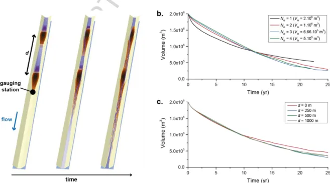
After large earthquakes, rivers are likely to receive sediments from multiple co-seismic landslides. Here, we investigate the impact of a cascade of landslides on sediment transport and evacuation. Two scenarios are explored. In the first one, the total volume of sediment introduced in the river remains constant (i.e. 2.106 m3) but is distributed along the stream in a cascade of 1 to 4 landslides separated by the same apex to apex distance. In the second one, we investigate the effect of the distance separating two individual landslides on the sediment evacuation dynamics. In both cases, sediment export is evaluated at the outlet of the most downstream landslide.
Figure 3 | Morphodynamic evolution of a reach evacuating several landslides. a. Snapshots of different stages of the Eros simulation. This is the case of 2 landslides of Vs = 1.10
6
ACCEPTED MANUSCRIPT
10
distance of d = 500 m. b. Evolution of the remaining sediment volume upstream of the ‘gauging station’ at constant total volume but for different number of individual landslides. Nls is the number of
landslides and Vls is the volume of those individual landslides. c. Evolution of the remaining sediment
volume upstream of the ‘gauging station’ for different distance (d) between the landslides.
In terms of morphodynamic evolution, the simulations with a cascade of landslide deposits (Fig. 2b and 3a) share similarities with those of single deposits. During the first stage, the landslides are large enough to create partial or total landslide dams. The lakes forming in between two deposits have zero transport capacity. Regressive erosion leads to the progressive and simultaneous incision into each landslide deposits by a river narrower than the width of the bedrock channel. Whereas sediments eroded from the most downstream landslide are rapidly evacuated, similarly to the simulation with one landslide, sediments from the upstream landslide enter the downstream lake and form a prograding delta that lasts until the lake is drained. The river eventually incises vertically into both deposits until it reaches the bedrock surface and then removes the remaining volume of sediment by lateral erosion.
When multiple landslide deposits enter the channel, the cases where Nls ≥ 2 display similar
export rates (Fig. 3b). Differences arise when these cases are compared with the evacuation of a single large landslide. In the latter, the landslide evacuation is more efficient until ~70% of the deposit is evacuated. The period of river increased efficiency (i.e. when the alluvial river width is less than 40% the one of the bedrock width) is also longer (Croissant et al, 2017). We then vary the inter-landslide distance 𝑑 to 0, 250, 500 and 1000 m. The results show that the distance between successive landslides appears to play only a minor role in the efficiency of total sediment evacuation. When we examine landslides individually (by setting gauging stations downstream of each deposit), however, the downstream landslides are evacuated less efficiently than those upstream, especially during the phase of lateral erosion (see Supplementary Figure S1). This is because the high sediment fluxes from the evacuation of the upstream landslides slows down the erosion of those downstream as the river is already loaded with sediment. Apart from this effect, the time-evolution of sediment transport for individual landslides remains relatively similar when considering a cascade of landslides or a single landslide. Taken together, when viewed from the downstream gauging station, the overall sediment
ACCEPTED MANUSCRIPT
11
export response of a cascade of landslides is similar to that of a single landslide in these single channel experiments (Fig. 3).
We, therefore, assume in the following discussions that the removal of landslides can be considered independently from each other. This assumption represents a critical step in building an upscaling approach where thousands of landslides can be triggered simultaneously in the river stream.
3. A reduced-complexity model for the export of landslide sediment
Earthquakes generally trigger numerous landslides that will eventually reach the fluvial network at locations with varying local transport capacity. As such, a cluster of landslides can be described as a distribution of the ratio 𝑉𝑙𝑠/𝑄𝑇 (Croissant et al., 2017) spanning the studiedend-members in the previous section. Whereas morphodynamic modelling provides useful information on the mechanisms of landslide removal at the reach scale, it is still too computationally demanding to apply it at the scale of a whole mountain range over hundreds to thousands of years and to accounting for thousands or more landslides. Therefore, we aim here to define a reduced-complexity model to describe the post-seismic evolution of landslide volume for any value of 𝑉𝑙𝑠/𝑄𝑇, informed by the
results obtained with 80 simulations performed in the previous section for the single landslide scenario.
Using these simulations, we compute the time 𝑇𝑒𝑥𝑝 needed to export 20 to 90% of the initial
𝑉𝑙𝑠 as a function of 𝑉𝑙𝑠/𝑄𝑇 at a 10% percent interval (Fig. 4a). As described in Croissant et al, 2017,
the export time computed for each interval follows a trend with 𝑉𝑙𝑠/𝑄𝑇 that can be fitted with a
function of the form:
𝑇𝑒𝑥𝑝,𝑖 = 𝛿𝑖(𝜇𝑖 𝑉𝑙𝑠 𝑄𝑇 ) [1 + (𝑉𝑙𝑠 𝑄𝑇 ) 𝜑𝑖 ] (𝛽−1) 𝜑𝑖 (5)
with 𝛿 and 𝜇 constants, 𝜑 a curvature parameter, 𝛽 an exponent (here fixed at 0.1) and 𝑖 corresponds to the studied percent interval. The values of these parameters are found by a least-square fitting using equation 5 on each percent interval (Fig. 4a, Table 1).
ACCEPTED MANUSCRIPT
12
We obtain a discrete description of the evolution of a landslide volume for any value of 𝑉𝑙𝑠/𝑄𝑇 (Fig. 4b, c). The continuous description is obtained by interpolating linearly between the
points.
Following this, the temporal evolution of landslide sediment evacuation can be assessed for two values of 𝑉𝑙𝑠/𝑄𝑇 which represent two end-members responses (Fig. 4b, c). Simulations
presenting a high 𝑉𝑙𝑠/𝑄𝑇 ratio never succeed to evacuate 100% of the initial volume of sediment as a
small fraction of sediment remains captured in lateral terraces. Therefore, to reconstruct fully the landslide export, we assume that the last 10% of sediment volume is exported at the same rate as that estimated for the last 20% to 10%. This may lead to a slight over-estimation of the efficiency of sediment transport during the lateral erosion phase.
This reduced-complexity method provides a computationally efficient way to appraise the post-seismic sediment evolution of landslide clusters. It also has the advantage of implicitly accounting for the evolution of the width and slope of the river. This reduced-complexity description of sediment export can, therefore, be applied at a larger spatial scale (i.e. a mountain range) provided that the distribution of 𝑉𝑙𝑠/𝑄𝑇 is known. In the next section, we combine this method with a newly
developed large-scale model, Quakos, which determines clusters of earthquake-triggered landslides, including the volume and the transport capacity of the river that they are connected to.
Figure 4 | Predicting the dynamic evacuation of landslides using Eros results. a. Series of fitting functions applied to predict the landslide export when x% of it has been evacuated. b. and c. Comparison between our predictions (yellow dots, green line) and Eros output (grey line) for 2 values of 𝑉𝑙𝑠/𝑄𝑇.
ACCEPTED MANUSCRIPT
13
4. Upscaling to sediment fluxes at the mountain range scale during several
seismic cycles
Here, we propose a statistical approach to quantify post-seismic sediment fluxes at the scale of a mountain range. Quakos is composed of three main components that can be used independently (Fig. 5a): 1. a statistical earthquake generator; 2. a landslide generator that predicts the 2D distribution of co-seismic landslides and the volumes using empirical laws; 3. a sediment evacuation model based on the reduced-complexity method described in previous section. The values of the parameters used in this section can be found in Table 2.
4.1. Model description
4.1.1. Study area
In the following, we consider a hypothetical failure of the Alpine Fault in the Southern Alps, New Zealand as a case study (Fig. 5). The formation of the Southern Alps and its recent morphologic evolution has occurred under extreme tectonic and climatic forcing (Tippett & Kamp, 1993). The rapid rate of convergence is largely accommodated by the Alpine Fault (Norris et al., 1990) which paleo-seismic studies have shown ruptures in large earthquakes (Mw > 7.5) with a recurrence time of
263 ± 68 years (Berryman et al., 2012; Cochran et al., 2017; Howarth et al., 2012). The` range of the Southern Alps extends ~450 km from southwest to northeast and rises from sea level to 3724 m at Mount Cook. It forms a natural barrier to western winds which leads to high rates of precipitation up to 13 m.yr-1 along the west coast (Tait & Zheng, 2007). Landscapes in the Southern Alps are characterized by steep hillslopes with modal values averaging at 35° (Korup et al., 2010) and are prone to landsliding even during aseismic periods (Hovius et al., 1997). Thousands of landslides are expected to be triggered in the next large seismic event, potentially mobilizing ~1 km3 of sediment (Marc et al., 2016; Robinson et al., 2016).
The topography of the Southern Alps is obtained from the SRTM3 digital elevation model (DEM), with a pixel size set at 100 m. Computations involving operations on the DEM have been performed using TopoToolbox_v2 (Schwanghart & Scherler, 2014).
ACCEPTED MANUSCRIPT
14
4.1.2 Fault, earthquakes and peak ground acceleration
Here, we design a thrust fault of length FL = 400 km and width FW = 19 km with a dipping
angle of 60° that approximatively mimics the geometry of the Alpine Fault (Robinson et al., 2016). In the Quakos model, earthquakes (mainshocks and aftershocks) are generated on this fault. When mainshocks are generated the ruptures cover the entire fault width, leading to earthquakes of magnitude Mw = 7.9. The position of each mainshock is randomly sampled along the fault plane. Each
mainshock triggers a series of aftershocks, which location, date and magnitude are determined using the BASS model (Turcotte et al., 2007). The aftershocks series are generated following three statistical laws:
- The difference between the magnitude of the mainshock and its largest associated aftershock (∆Mw = 1.25) is determined using a modified version of Båth’s law
(Shcherbakov et al., 2004).
- The rate of aftershocks is submitted to a temporal decay described by a generalized form of Omori’s law (Shcherbakov et al., 2004). Parameters from this law are the exponent p = 1.25 and offset c = 0.1 days.
- The spatial distribution of aftershocks is given by a spatial form of Omori’s law (Helmstetter & Sornette, 2003) with the exponent q = 1.35 and offset d = 4 meters. All the defined parameter values of the BASS model are taken from Turcotte et al., [2007] and are constant for all the simulations performed in this paper.
The range of simulated magnitudes is bounded by fault dimensions, for the largest magnitude, and by the spatial discretization of the fault, for the smallest magnitude. Simulated earthquakes have magnitudes ranging from 2.5 to 7.9. For each earthquake (mainshocks and aftershocks), the associated rupture length (𝑅𝐿) and width (𝑅𝑊) are estimated as a function of seismic moment, 𝑀𝑂 following a
consistent set of scaling laws based on empirical observations determined for strike-slip faults (Leonard, 2010): 𝑅𝐿= ( 𝑀𝑂 𝜇𝐶13 2⁄ 𝐶2 ) 𝛽 (6)
ACCEPTED MANUSCRIPT
15
𝑅𝑊 = 𝐶1𝑅𝐿𝛿 (7)
where 𝜇 = 33 GPa is the shear modulus and 𝐶2 = 3.6.10-5, 𝐶1, 𝛽 and 𝛿 are constants which value
depends on the rupture length:
- 𝑅𝐿 < 5 km: 𝐶1 = 1, 𝛽 = 1/3 and 𝛿 = 1.
- 5 km < 𝑅𝐿< 45 km: 𝐶1 = 15, 𝛽 = 2/5 and 𝛿 = 2/3.
- 𝑅𝐿 > 45 km: 𝐶1 = FW, 𝛽 = 2/3 and 𝛿 = 1.
For a given earthquake, a map of the synthetic peak ground acceleration (PGA) is computed as a function of earthquake magnitude, ruptured fault geometry (rake, dip, dimension), fault mechanism, lithological controls and site effects (Fig. 5b) (Campbell & Bozorgnia, 2008). The theoretical framework that derives from this work is quite extensive (see equations 1 to 12 in Campbell & Bozorgnia, [2008]). Here, we consider the sediment depth Z2.5 = 0 m, a S-wave velocity
in the first 30 m of the crust Vs,30 = 180 m.s
-1
and a reference PGA at Vs = 1100 m.s
-1
, A1100 = 0.10 g
(Robinson et al., 2016). For other parameter values, we refer to Table 2 in Campbell & Bozorgnia, [2008].
ACCEPTED MANUSCRIPT
16
Figure 5 | Quakos workflow used to predict landsliding pattern at the mountain range scale. a. Quakos workflow. b. PGA pattern predicted by the model for a Mw 8 scenario on the Alpine Fault,
New Zealand. c. Map of the landslide density. d. Landslide pattern predicted by Quakos. The view is focused on catchments located on the Central Southern Alps. Yellow dots indicate landslides, the sizes are a function of landslide area. White dots outside of the considered catchments only represent the location of landslides. Notation: Vls, landslide volume.
4.1.3 Landslides triggered by earthquakes
Modelled maps of PGA are then used to infer the spatial density of triggered landslides, i.e. the number of landslides by unit area. Previous studies suggest that the density of earthquake-triggered landslides is linearly dependent on the PGA (Meunier et al., 2007; Yuan et al., 2013):
ACCEPTED MANUSCRIPT
17
𝑃𝑙𝑠= 𝛼𝑝𝑃𝐺𝐴 − 𝛽𝑝 (8)
where 𝛼𝑝 and 𝛽𝑝, are two empirical parameters that controls the maximum density of landslide and
its spatial repartition, respectively. The parameter 𝛽𝑝 is a critical value of PGA under which no or
very few landslides are triggered. The values of these parameters are highly dependent on the studied case and the choice of their value is explained in the result section. Following the work of Meunier et al., [2007], locations where the local slope is less than 20% (on a 100m DEM) are not affected by landsliding. In our case study, this mostly prevents landslides from being triggered on alluvial fans and large river valleys (Fig. 5c, d).
The area distribution of earthquake-triggered landslides is commonly given by an inverse gamma probability density function:
𝑝𝑑𝑓(𝐴𝑙𝑠) = 1 𝑎𝛤(𝑎)[ 𝑎 𝐴𝑙𝑠− 𝑠 ] 𝜌+1 𝑒𝑥𝑝 [− 𝑎 𝐴𝑙𝑠− 𝑠 ] (9)
with 𝑎 a parameter controlling the position of the pdf maximum, 𝑠 a parameter controlling the roll-over for small landslides and 𝜌 is a positive exponent controlling the tail of the pdf (Malamud et al., 2004a). In Quakos simulations, the area of each landslide belonging to a landslide cluster is determined by randomly sampling the 𝑝𝑑𝑓(𝐴𝑙𝑠). The location of landslides is then determined
according to the map of landslide density (Fig. 5d). At this stage, those two conditions are met and then landslides are distributed randomly on slopes above >20%. Future improvements to this approach may include methods to preferentially select parts of the landscape where landslides locate, and link this to the morphology of the local hillslopes at the ~ km2 scale.
For each individual predicted landslide, its planform area is converted to volume 𝑉𝑙𝑠 by using an
empirical scaling law:
𝑉𝑙𝑠 = 𝛼𝐴𝑙𝑠 𝛾
(10) with 𝛼 and 𝛾 are set to 0.05 and 1.5 (Hovius et al., 1997; Larsen et al., 2010). This parameterization is well-suited to infer the volume of deep-seated bedrock landslides which dominate the volume budget of a population of triggered-landslides.
ACCEPTED MANUSCRIPT
18
After Quakos has provided a distribution of earthquake-triggered landslides, the prediction of post-seismic landslide evacuation depends mostly on: 1. the rate of sediment supply to the channel network, i.e. the transfer of material from hillslopes to channels, and 2. the rate of sediment transport by the river.
Several studies have pointed out the importance of the initial and dynamic connectivity of landslides to the channel network on post-seismic sediment fluxes (Li et al., 2016; Roback et al., 2018). Some studies provide an estimation of initial connectivity ranging from 8% to 43 % and even to full connectivity (Dadson et al., 2004; Li et al., 2016; A. J. West et al., 2011). Based on the data of Li et al [2016] and Roback et al., [2018], the initial landslide-channel connectivity 𝐶 of each landslide is determined as a function of its area 𝐴𝑙𝑠:
𝐶 = 𝑚𝐴𝑙𝑠,𝑏𝑖𝑛𝜔 (11)
where 𝑚 is an empirical constant and 𝜔 an empirical exponent (see Supplementary Figure S3). Equation (11) applies for landslides presenting an area lower than 1.106 m2. Above this threshold, we assume that landslides are always initially connected to the drainage network. This assumption is supported by empirical data and because larger landslides usually present a longer run out (Lucas et al., 2014). Here, 𝐶 gives the percentage of connected landslides in the considered bin of landslide area (𝐴𝑙𝑠,𝑏𝑖𝑛) on a logarithmic scale.
To consider landslide deposits which locate away from the channel network on steep slopes, we consider that transport of loose debris is likely to occur at a velocity that likely depends on the climatic and meteorological context and local topographic properties. Unfortunately, studies which quantify the post-seismic sediment delivery from hillslopes to channels are scarce because of the difficulties of measuring it in the field or using remote sensing (Fan et al., 2018; Zhang et al., 2016).
We, therefore, develop a simplified approach to account for a “dynamic connectivity” of landslides to rivers. This approach first determines the distance (𝑑) between the landslide and the closest river connection point using a steepest descent algorithm. The timing of connection is then obtained by setting a constant and arbitrary connectivity velocity (𝑢𝑐𝑜𝑛) to each landslide and
computed as 𝑡𝑐𝑜𝑛 = 𝑑/𝑢𝑐𝑜𝑛 . Once the landslide is connected to the river network, we assume that
ACCEPTED MANUSCRIPT
19
modification may be to link this dynamic connectivity to diffusive erosion processes which occur on steep surfaces (Roering et al., 1999). Here, for simplicity, we first explore scenarios with a constant 𝑢𝑐𝑜𝑛.
Once a landslide reaches the closest stream, its subsequent evacuation depends on the ratio between its volume 𝑉𝑙𝑠 and the local river transport capacity 𝑄𝑇 following equation (5). If the
landslide volume is determined for each landslide using Quakos, the transport capacity needs to be computed. The along-stream transport capacity of bedrock rivers is set by its geometry (width and slope), local river discharge and sediment grain size. The bedrock river width (𝑊), slope (𝑆) and mean discharge (𝑄̅) are expressed as a function of the local drainage area (𝐴) as:
{
𝑊 = 𝑘𝑤𝑛𝐴0.5
𝑆 = 𝑘𝑠𝑛𝐴−0.45
𝑄̅ = 𝑟̅𝐴
(12)
with 𝑘𝑤𝑛 the normalized width index, 𝑘𝑠𝑛 the normalized steepness index and 𝑟̅ mean annual runoff
(Lague, 2014). Here, the critical drainage area used to extract the drainage network is equal to 0.5 km2.
To ensure the same context as the Eros simulations, the river transport capacity is described using an effective daily discharge (Qeff) presenting a return time of one year which is a good
compromise between frequency of occurrence and the amount of geomorphic work of such events. The bedload transport capacity (Meyer-Peter & Müller, 1948) is then computed as:
𝑄𝑇 = 𝑊𝐾 (𝜌𝑤𝑔 ( 𝑛𝑄𝑒𝑓𝑓 𝑊 ) 0.6 𝑆0.7− (𝜌𝑠− 𝜌𝑤)𝑔𝜏𝑐∗𝐷50) 1.5 (13) with 𝜏𝑐∗ the critical Shields stress, 𝜌𝑤 the water density, 𝜌𝑠 the sediment density, 𝑛 the Manning
friction coefficient, 𝐾 an erodability constant and 𝑔 the gravitational constant. For simplicity, the grain size distribution of the landslide is reduced to the median grain size descriptor 𝐷50 which is
chosen to be constant for all landslides.
To compute the value of Qeff, we assume that the range of daily discharges 𝑄, experienced at
any point along the river, follows an inverse-gamma probability density function:
𝑝𝑑𝑓(𝑄) = 𝑘 𝑘+1 𝛤(𝑘 + 1)𝑒𝑥𝑝 (− 𝑘 𝑄/𝑄̅) (𝑄/𝑄̅) −(2+𝑘) (14)
ACCEPTED MANUSCRIPT
20
with 𝛤 the gamma function and 𝑘 a parameter linked to the variability of the hydrological forcing, here, fixed at k = 1, based on empirical data (Croissant et al., 2017; Lague et al., 2005). This assumption is supported by empirical data, that demonstrate that the runoff of rivers located along the West Coast of New Zealand present a high variability (k = 1) (Croissant et al, 2017b). From this distribution, the return time (𝑡𝑟) of a particular daily discharge can be assessed using:
𝑡𝑟(𝑄𝑒𝑓𝑓) = 𝛤(𝑘/𝑄𝑒𝑓𝑓, 𝑘 + 1)−1 (15)
The value of Qeff can be computed using this equation.
4.2 Landslide triggering and sediment export over a seismic cycle
4.2.1 The volume of triggered landslides by earthquakes on the Alpine Fault
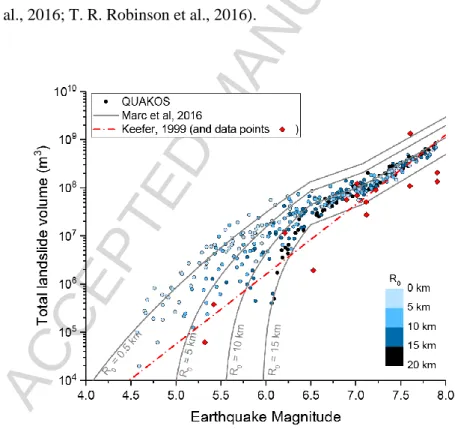
To assess Quakos outputs, we compare them to natural observations and existing analytical models (Keefer, 1999; Odin Marc et al., 2016). We plot the total volume of landslide clusters as a function of earthquake magnitude (Fig. 7). Consistent with Marc et al, [2016], Quakos leads to a threshold magnitude, here ~4.5, under which no landslides are generated. This threshold results from the fact that landslides are only generated if a critical PGA is reached (eq. 6; see Supplementary Movie S1). Above this threshold, the total landslide volume triggered by an earthquake increases with magnitude and shows a sensitivity to the depth of earthquake nucleation. The variability of total landslide volume for earthquakes of equal magnitude results from the depth of the earthquake but also from the variability of the topography impacted by landsliding, including the proportion of the topography with local slopes greater than 20%. For low magnitudes, total landslide volume is strongly sensitive to the depth of the earthquake. Indeed, the width extent of the rupture is small compared to fault width, and the depth of the earthquake becomes the controlling factor to generate PGA above the critical value for landsliding. This mostly explains the spread in the distribution of total landslide volume as a function of magnitude for earthquakes with magnitude lower than ~6.5. Larger earthquakes are less prone to this spread in total landslide volume as the rupture width becomes closer to fault width. We also note that Quakos outputs asymptotically tend, for large magnitudes, towards the analytical model from Marc et al, [2016] for R0 = 15 km, independently from Quakos depth of theACCEPTED MANUSCRIPT
21
& Bozorgnia, 2008), covering the entire fault width for the largest earthquakes, and not on the depth of the earthquake. Whereas Marc et al. [2016] only consider the depth of the sources of seismic waves, and not the rupture extent. Total landslide volume is also sensitive to the parameters in equations 8 and 9, which control the number of triggered landslides for a given PGA and their volume distribution (see supplementary Figure S2).
For a Mw 7.9 earthquake occurring on the Alpine Fault, without considering aftershocks, the
total number of landslides generated in the Southern Alps is ~17700 ± 500 landslides with a total volume of sediment 0.75 ± 0.07 km3 (Fig. 6). Empirical constraints allow for a more accurate estimation of the characteristics of a future earthquake on the Alpine Fault.The total number of landslides, however, is of the same order of magnitude as most of the natural cases documented in Tanyaş et al., [2017] and the total volume is similar to the one estimated by two independent studies (Odin Marc et al., 2016; T. R. Robinson et al., 2016).
Figure 6 | Relationship between the total volume of landslides triggered by earthquakes and the magnitude, in the case of a strike-slip fault. Quakos results (circles) are coloured as a function of the depth of the earthquake compared to the surface (R0). Quakos outputs are compared to two
empirical models from Marc et al, [2016] and Keefer, [1999].
ACCEPTED MANUSCRIPT
22
Here, we explore the dynamic of sediment export over a single seismic cycle that follows a
Mw 7.9 earthquake. We only consider the river catchments of the West Coast where the landslide number is ~12000 and total volume is ~0.5 km3. We focus on the role of the initial and dynamic connectivity of landslides to the fluvial network in controlling post-seismic sediment evacuation. Based on the morphodynamic modelling results, we assume that landslides located in the same river reach are evacuated independently of each other.
At the initial stage, ~41% of the total volume of landslide sediment is connected to the drainage network. Models with 𝑢𝑐𝑜𝑛 equals to 0.1, 1 and 10 m.yr-1 lead to 43, 50 and 96% of the total
volume evacuated over 263 years. The ‘full connectivity’ case leads to the highest rates of sediment transport with 70% of the landslide mass evacuated in less than 10 years (Fig. 7a). This value matches to order of magnitude the predictions of Croissant et al, [2017] for high mean annual runoff and runoff variability and for which the full population of landslides was assumed fully connected. After 2000 years, most of the sediment volume is removed for 𝑢𝑐𝑜𝑛 ≥ 1 m.yr-1, whereas the rivers are
starved of sediments because of the absence of new connected landslides for 𝑢𝑐𝑜𝑛 = 0.1 m.yr-1. This
illustrates, that landslide connectivity is an important factor limiting sediment evacuation after the triggering of landslides by a large earthquake. In turn, landslide connectivity is critical to assess the fraction of co-seismic debris evacuated before the next earthquake occurs.
ACCEPTED MANUSCRIPT
23
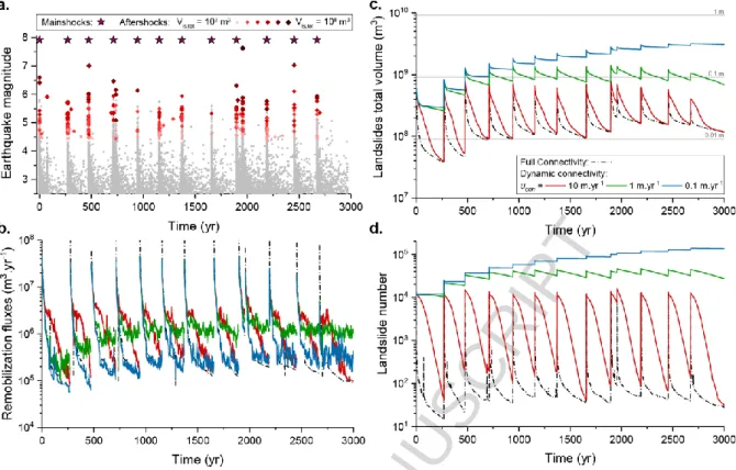
Figure 7 | Temporal evolution of the Mw 7.9 earthquake simulations with different connectivity
properties. a. Temporal evolution of the landslide volume for different connection velocities. b. Temporal evolution of the number of landslides. c. Sediment remobilization fluxes. d Temporal evolution of the number of active landslides, i.e. landslides that are being connected to the drainage network and being actively evacuated by the river. Note: The grey area indicates the estimated return time of a Mw 8 earthquake on the Alpine Fault.
Interestingly, the number of active landslides (Fig. 7d), i.e. connected landslides with remaining sediments, do not exactly follow the total landslide volume evolution (Fig. 7a). This occurs because the volume of deposits in the landscape is controlled by the largest landslides. For low values of 𝑢𝑐𝑜𝑛, model predictions show that a large proportion of the initial landslide population can be
preserved while having evacuated a moderate to large proportion of the volume of earthquake-produced sediment (Fig. 7b).
Connectivity also impacts the amplitude and duration of the rates of sediment remobilization (Fig. 7c). The full connectivity case presents rates that are at least one order of magnitude greater than any other model during the first years after the earthquake. This rate drops abruptly by three orders of magnitude in less than a century. On the contrary, for 𝑢𝑐𝑜𝑛 < 10 m.yr-1, the the rate of remobilization
oscillates during the first 200 years before decreasing progressively. The different rates are controlled by the sediment delivery from hillslope to the channels (Fig. 7d). A low value of 𝑢𝑐𝑜𝑛 ensures a
ACCEPTED MANUSCRIPT
24
progressive and near-constant delivery of sediment with a steady number of landslides being active during the first 200 years.
Figure 8 | Probability density function of landslide volumes at different time steps. a. For the Full connectivity case. b. For the case 𝑢𝑐𝑜𝑛 = 10 m.yr-1. c. For the case 𝑢𝑐𝑜𝑛 = 1 m.yr-1.
The velocity of connection has also an impact of the evolution of the distribution of landslide volume (Fig. 8). We here account for the volume changes as landslide are being evacuated by river sediment export. For the full connectivity case, the temporal evolution of the probability density function (pdf) of landslide volume, pdf(Vls), shows that landslides with volumes smaller than 10
3
m3 disappear from the distribution after only five years as they tend to have characteristic timescales 𝑉𝑙𝑠/𝑄𝑡 < 1 year. Over longer durations, the remaining landslides tend towards the largest areas and the
distribution shrinks towards these largest areas. There is however no change in the scaling of the tail of the pdf(Vls). For 𝑢𝑐𝑜𝑛 = 10 m.yr-1 the shape of the pdf is preserved during 50 years until the largest
landslides start to dominate the long-term signal (Fig. 8b). Moreover, the slope of the tail of the pdf changes with time and becomes less steep. This occurs because of the parametrization of the initial connectivity in Equation (11) which favors the connection of large landslides and tend to preserve small landslides. For 𝑢𝑐𝑜𝑛 ≤ 1 m.yr-1, and probably also for lower values of 𝑢𝑐𝑜𝑛, the shape of the
pdf is preserved through time. This occurs because only a very limited fraction of the landslide population is actively connected to the fluvial network, and most landslides are preserved within the mountain range.
ACCEPTED MANUSCRIPT
25
4.3 Upscaling to several seismic cycles
In this section, we extend model duration to several seismic cycles. The scenario is chosen to mimic the response observed on the Alpine fault, i.e. a temporal series of 12 Mw = 7.9 mainshocks
separated by recurrence period randomly sampled in the 263 +/- 68 years range (Fig. 9). The production of co-seismic landslides is slightly different for each mainshocks, because ofthe stochastic way in which Quakos simulates individual landslide areas and volumes, with a total volume ~0.45 m3 and an average total number of landslides of 13000 on the West Coast.
Each mainshock is followed by a series of aftershocks with magnitudes varying between 2.5 and 7.5, some of which mobilise an additional volume of sediment. In most cases, the contribution of aftershocks is generally lower than that of mainshocks for two reasons: 1. they mobilize sediment volumes that are lower by 1 to 5 orders of magnitude (Fig. 9a) and 2. most of landslide-triggering aftershocks are quasi-synchronous with mainshocks and, therefore, the total sediment production is dominated by the one of the mainshock. Aftershocks occurring between two mainshocks, however, can have a visible impact on the sediment production as highlighted by the Mw 7.5 earthquake at
ACCEPTED MANUSCRIPT
26
Figure 9 | Temporal upscaling over several seismic cycles. a. Times series of earthquakes generated on the faults. It is characterised by a series of mainshocks of Mw = 7.9 followed by the
sequences of aftershocks. The dot size and color are a function of the total volume of the landslide population (Vls,tot). The grey dots indicate earthquakes that have not triggered any landslides. b.
Evolution of the remobilization fluxes. c. Evolution of the total volume of sediment mobilized by the successive earthquakes. Grey lines represent the mean sediment thickness that would be deposited on the total area affected by landsliding. d. Evolution of the number of landslides in the mountain range.
Over the 12 seismic cycles, rivers are never able to export all the earthquake-mobilized sediment (Fig. 9c). Yet, they progressively reach a dynamic steady-state between new sources of sediment, because of landslide triggering during earthquakes, and sediment evacuation of all the previous generation of co-seismic landslides. The duration of the transient phase and the average volume of sediment remaining in the mountain at steady-state is controlled by 𝑢𝑐𝑜𝑛. For 𝑢𝑐𝑜𝑛 ≥ 10
m.yr-1 the steady-state is reached after three seismic cycles with a sediment storage within the mountain range reaching a minimum of 10-20% of one Mw 7.9 earthquake worth of sediment. Most of
the landslides are evacuated within one seismic cycle reaching a minimum of 50-100 landslides remaining in the catchments (Fig. 9d). For 𝑢𝑐𝑜𝑛 ≤ 1 m.yr-1, the earthquake-produced sediment
progressively piles-up inside the mountain range, stored on hillslopes, until an equilibrium situation is reached after 1500 years in which only a small proportion of the newly triggered population is removed. In these cases, the sediment volume that is stored within the mountain range at the end of
ACCEPTED MANUSCRIPT
27
each seismic cycle is equivalent to 120% (𝑢𝑐𝑜𝑛 = 1 m.yr-1) to 600% (𝑢𝑐𝑜𝑛 = 0.1 m.yr-1) of the average
value of earthquake-triggered initial landslide volume. These cases are also characterized by the persistence of several thousands of landslides in the mountain range.
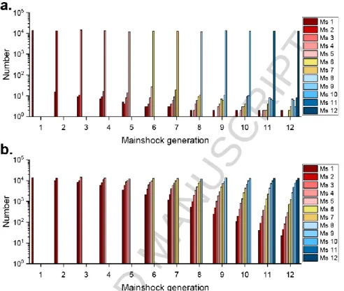
Figure 10 | Landslide generations. a. For the Full connectivity case. b. For the case ucon = 1 m.yr -1
. Notation: Ms: mainshocks.
Figure 10 shows the repartition of landslides generation at the occurrence of each mainshocks. The repartition is dominated, unsurprisingly, by the i-th generation of landslides at the time of occurrence of the i-th mainshock. Despite that, the full connectivity case (Fig. 10a) shows that only a few landslides of early generations are preserved over tens of seismic cycles. This is illustrated by the presence of two landslides of the 1-th generation at the occurrence of the 12-th mainshock. Because no dynamic connectivity occurs in this case, this persistence is explained by rare landslides characterized by very low transport capacity and very high 𝑉𝑙𝑠/𝑄𝑡. For low velocities of connection
(Fig. 10b), preservation of landslides over tens of seismic cycles becomes less exceptional. This is illustrated by the wide diversity of generations of landslides preserved when the last mainshock occurs.
ACCEPTED MANUSCRIPT
28
Figure 11 | a. Time necessary to evacuate a landslide cluster as a function of mean annual runoff and connection velocity. Black lines represent a 𝑡𝑒𝑥𝑝 value of 25, 50 and 75 % of the duration of a seismic
cycle. b. Relative importance of the two timescales controlling post-seismic landslide evacuation. Based on the results of Figure 9, we aim to define a representative export time of the sediment delivered by the whole population of earthquake-triggered landslides. This index is based on the two intrinsic timescales that are involved in these simulations: 1. the time, 𝑡ℎ𝑖𝑙𝑙, necessary to transfer
landslide material from hillslopes to channels by dynamic connectivity and 2. the time, 𝑡𝑟𝑖𝑣,
necessary to transport landslide sediment by the river network. 𝑡𝑟𝑖𝑣 is computed as the time necessary
to remove 90% of the total landslide volume for different mean annual runoff intensity under the assumption that all the landslides are connected. 𝑡ℎ𝑖𝑙𝑙 is computed as the mean connection time of the
whole landslide population:
𝑡ℎ𝑖𝑙𝑙=
∑𝑁𝑗=1𝑙𝑠 𝑉𝑙𝑠,𝑗𝑡𝑐𝑜𝑛,𝑗
∑𝑁𝑗=1𝑙𝑠 𝑉𝑙𝑠,𝑗
(16)
With 𝑁𝑙𝑠 the number of landslides, 𝑉𝑙𝑠,𝑗 and 𝑡𝑐𝑜𝑛,𝑗 the volume and connection time of the j-th
landslide. We then compute the mean export time 𝑡𝑒𝑥𝑝 of the landslide population normalized by the
average duration of the seismic cycle 𝑇𝑠−𝑐:
𝑡𝑒𝑥𝑝 =
𝑡ℎ𝑖𝑙𝑙+ 𝑡𝑟𝑖𝑣
ACCEPTED MANUSCRIPT
29
The mean export time of the landslide population increases when decreasing the mean annual runoff and or the connection velocity 𝑢𝑐𝑜𝑛 (Fig. 11a). 𝑡𝑒𝑥𝑝 is lower than one seismic cycle for 𝑢𝑐𝑜𝑛
greater than 2 m.yr-1, except when the mean annual runoff becomes close to 2 m.yr-1, the critical runoff below which no sediment transport occurs. For a mean annual runoff greater than 3 m.yr-1
and
𝑢𝑐𝑜𝑛 lower than 2 m.yr-1, 𝑇𝑒𝑥𝑝 is almost independent of the mean annual runoff. For this regime
sediment export is limited by connectivity as 𝑇ℎ𝑖𝑙𝑙 is greater than 𝑇𝑟𝑖𝑣 and the rivers are lacking
sediments (Fig. 11b). This highlights the importance of hillslope processes in controlling the export time of a landslide population. When 𝑢𝑐𝑜𝑛 is greater than 10 m.yr-1, sediment export is limited by
river transport as 𝑇ℎ𝑖𝑙𝑙 is lower than 𝑇𝑟𝑖𝑣 and the rivers are loaded by sediments. The limit between the
connectivity- and transport-limited regimes tends towards lower values of 𝑢𝑐𝑜𝑛 when the mean annual
runoff gets closer to its critical value around 2 m.yr-1.
5. Discussion
Our theoretical modelling approach emphasizes the need to integrate various processes involved in the production and routing of co-seismic landslide debris across several seismic cycles, partly at the expense of individual process complexity. An important novelty is the spatially explicit nature of peak ground acceleration, co-seismic landslide and transport, and the inclusion of important channel morphodynamic feedback occurring for large landslides. Yet, our model is based on several assumptions. We still have a rather limited understanding and/or lack of empirical data for three key processes: generation of co-seismic landslide, landslide connectivity and hillslope transfer, and river morphodynamics. Here, we discuss these limitations and highlight challenges to overcome.
5.1 Generation of co-seismic landslides
Compilations of empirical datasets show that co-seismic landslide cluster properties (total volume, area and number) exhibit large variations which mainly depend on the tectonic forcing and the topographic properties of the affected mountain range (Tanyaş et al., 2017). Early work has shown that these properties are primarily correlated to earthquake magnitude (Keefer, 1994). Other studies
ACCEPTED MANUSCRIPT
30
have improved this analysis by accounting for seismological characteristics and important topographic attributes to provide a seismologically-consistent model (Marc et al., 2016). No theoretical framework, however, is robust enough to predict with accuracy what would be the properties (volume and localisation) of a landslide cluster for a future event. In our modelling approach, we build on the previous work by using a PGA-dependent model that also accounts for topographic properties to generate co-seismic landslide clusters. The novelty of this approach relies on predictions of spatialized landslide distributions within a mountain range while being consistent with previous empirical data and analytical model. An accurate prediction of landslide cluster properties is important because several components of the post-seismic sediment evacuation depend on them, i.e. the dependency of initial connectivity to landslide area and export time to landslide volume (see Supplementary Figure S2 and S4).
In our approach, Quakos generates earthquake-triggered landslide clusters with a spatial density that linearly depends on PGA (Meunier et al., 2007). Slope, curvature, and distance from ridges are identified as other controlling parameters of landslide initiation (Meunier et al., 2008; Robinson et al., 2017; Tanyas et al., 2019). Yet, to date, no consensus exists on a theoretical framework to accurately predict the spatial distribution of earthquake-generated landslides (Reichenbach et al., 2018). A common theme of these assessments is that they rely primarily on the PGA patterns and have to be calibrated against a pre-existing partial co-seismic landslide catalogues. These are non-existent for the Alpine Fault. Accounting for more detailed model of landslide susceptibility would have an impact on the landslide distances to stream distribution and then on the dynamic connectivity. In addition, in our modelling approach the maximum value of the landslide density is limited by the transport capacity computed at the outlet of catchments. Indeed, the sum of sediment volume exported out of connected landslides within one catchment cannot be greater that the transport capacity at the catchment outlet.
We have also assumed that the generation of co-seismic landslide is independent of the state of landslide export from previous events. This is a reasonable assumption in the transport-limited regime, but the accumulation of co-seismic material on hillslopes in the connectivity-limited regime may at some point reduce the likelihood of landsliding. Similarly, the reactivation of co-seismic
ACCEPTED MANUSCRIPT
31
landslide is not accounted for in our approach (Marc et al., 2015) and may well contribute to further increase the release of debris in the channel network.
5.2 Evacuation of post-seismic landslide
A better understanding of the mountain range response to a sudden increase in sediment supply requires new data on 1. the initial landslide connectivity, 2. the processes controlling the debris transport dynamics on hillslopes and rivers and 3. The export of river sediment, including the partitioning between the production of fine and coarse sediment and its implication on the subsequent sediment evacuation. We discuss these three main points in the following.
5.2.1 Initial landslide connectivity
At the landscape scale, our results highlight the role of initial connectivity on the modulation of the sediment evacuation and export fluxes during the first few years that follow earthquakes (Fig. 7b). The assignment of an initial connectivity status to each landslide relies on only two empirical relationships between landslide area and connectivity (Li et al., 2016; Roback et al., 2018). The wide range of initial connectivity found in the literature, e.g. for earthquakes occurring in mountain ranges presenting different tectonic and climatic contexts, however, calls for a more systematic study of this process (Dadson et al., 2004; Li et al., 2016; West et al., 2011). The differences in tectonic and climatic settings lead to a variety of topographic configurations that could promote (or inhibit) initial connectivity and the subsequent sediment transfers from hillslope to channel. For instance, hillslope size, valley width, slope distribution, runoff distribution (frequency-magnitude) could all potentially impact the initial connectivity by controlling: 1. the abundance of large landslides with long runout, thus promoting a higher initial connectivity (see Supplementary Figure S2 and S3) 2. the distance required for the landslide to reach the nearest river and 3. the possibility of the river to erode vertically (narrow valleys) or horizontally the landslide deposits (wide valleys), the former being more efficient (Croissant et al., 2017).
ACCEPTED MANUSCRIPT
32 5.2.2 Dynamic landslide connectivity
Over centennial timescales, our modelling framework demonstrates that the distribution of connection times determines the efficiency at which earthquake-mobilized sediment is exported from a mountain range over a seismic cycle (Fig. 11). However, because of a lack of theoretical and empirical constraint, these results are based on a simple description of dynamic connectivity by a constant velocity which value varies on a large range encompassing two extreme behaviors. The ‘full-connectivity’ scenario implies the injection of the totality of landslides immediately during the co-seismic period leading to extremely high sediment fluxes. On the contrary, the lowest value of the connection velocities implies that most of the evacuated landslides are the one initially connected to the fluvial network, the remaining of the landslide population being stored on hillslopes during several seismic cycles.
Potentially, hillslope to channel material transfer could be described by more complex physical laws, such as a diffusion law (Roering et al., 2001) or transport laws relevant to colluvial processes (e.g., Lague and Davy, 2003). These laws would make the connection times dependent on the geometric properties of its path to the river (i.e. local slope) in addition of the distance to the stream. It would affect the distribution of connection times and therefore the dynamic of post-seismic landslide evacuation (see Supplementary Fig S6 and S7). However, mean climate variables (precipitation, temperature, vegetation growth, storms and co-seismic reactivation, remain difficult to include in these geomorphic laws. These limitations call for a better description of this process based on a more extensive collection of empirical data (Fan et al., 2018).
Given the large spatial scales (i.e. > 100 km) and the difficulties of measuring total sediment fluxes (i.e. suspended plus bedload) in the field, remote sensing is well-suited to track the post-seismic evolution of sediment masses (Scaioni et al., 2014). This can benefit from a variety of techniques to investigate landscape evolution in 2D (satellite imagery) and 3D (e.g., photogrammetry, laser scanning) and, thus, aim toward a detailed quantification of the system through time (Cook et al., 2018; Fan et al., 2018a; Jaboyedoff et al., 2012). An important issue over centennial timescales is a better understanding of the contribution of rare events to long-term dynamics. As remote sensing only gives a first order quantification of sediment mass transfer, a full understanding of the processes