HAL Id: hal-02965084
https://hal.archives-ouvertes.fr/hal-02965084
Submitted on 13 Oct 2020
HAL is a multi-disciplinary open access
archive for the deposit and dissemination of
sci-entific research documents, whether they are
pub-lished or not. The documents may come from
teaching and research institutions in France or
abroad, or from public or private research centers.
L’archive ouverte pluridisciplinaire HAL, est
destinée au dépôt et à la diffusion de documents
scientifiques de niveau recherche, publiés ou non,
émanant des établissements d’enseignement et de
recherche français ou étrangers, des laboratoires
publics ou privés.
Detection of a repeated transit signature in the light
curve of the enigma star KIC 8462852: A possible
928-day period
F. Kiefer, A. Lecavelier Des Étangs, A. Vidal-Madjar, G. Hébrard, V.
Bourrier, P. A. Wilson
To cite this version:
F. Kiefer, A. Lecavelier Des Étangs, A. Vidal-Madjar, G. Hébrard, V. Bourrier, et al.. Detection of
a repeated transit signature in the light curve of the enigma star KIC 8462852: A possible 928-day
period. Astronomy and Astrophysics - A&A, EDP Sciences, 2017, 608, pp.A132.
�10.1051/0004-6361/201731306�. �hal-02965084�
A&A 608, A132 (2017) DOI:10.1051/0004-6361/201731306 c ESO 2017
Astronomy
&
Astrophysics
Detection of a repeated transit signature in the light curve
of the enigma star KIC 8462852: A possible 928-day period
F. Kiefer
1, A. Lecavelier des Étangs
1, A. Vidal-Madjar
1, G. Hébrard
1, 2, V. Bourrier
3, and P. A. Wilson
1, 41 Institut d’Astrophysique de Paris, UMR 7095 CNRS, Université Pierre & Marie Curie, 98 bis boulevard Arago, 75014 Paris, France
e-mail: [email protected]
2 Observatoire de Haute-Provence, CNRS, Université d’Aix-Marseille, 04870 Saint-Michel-l’Observatoire, France 3 Observatoire de Genève, Chemin des Maillettes 51, Sauverny, 1290 Versoix, Switzerland
4 Leiden Observatory, Leiden University, Postbus 9513, 2300 RA Leiden, The Netherlands
Received 2 June 2017/ Accepted 2 September 2017
ABSTRACT
As revealed by its peculiar Kepler light curve, the enigmatic star KIC 8462852 undergoes short and deep flux dimmings at a priori unrelated epochs. This star presents nonetheless all other characteristics of a quiet 1 Gyr old F3V star. These dimmings resemble the absorption features expected for the transit of dust cometary tails. The exocomet scenario is therefore most commonly advocated. We reanalysed the Kepler data and extracted a new high-quality light curve to allow for the search of shallow signatures of single or a few exocomets. We discovered that among the 22 flux dimming events that we identified, two events present a striking similarity. These events occurred 928.25 days apart and lasted for 4.4 days with a drop in the star brightness by 1000 ppm. We show that the light curve of these events is well explained by the occultation of the star by a giant ring system or by the transit of a string of half a dozen exocomets with a typical dust production rate of 105–106kg s−1. Assuming that these two similar events are related to the transit of
the same object, we derive a period of 928.25 days. The following transit was expected in March 2017 but bad weather prohibited us from detecting it from ground-based spectroscopy. We predict that the next event will occur between 3−8 October 2019.
Key words. stars: individual: KIC 8462852 – techniques: photometric – comets: general – planets and satellites: rings
1. Introduction
KIC 8462852 is a peculiar and intriguing source that gar-nered a lot of attention from the astronomical community in the recent years (Boyajian et al. 2016; Marengo et al. 2015; Lisse et al. 2015; Schaefer 2016; Hippke et al. 2016; Abeysekara et al. 2016; Bodman & Quillen 2016; Lund et al. 2016; Thompson et al. 2016; Schuetz et al. 2016; Harp et al. 2016;Wright & Sigurdsson 2016; Montet & Simon 2016; Makarov & Goldin 2016; Neslušan & Budaj 2017; Ballesteros et al. 2018). KIC 8462852 is an F3V star located at about 454 ± 35 pc away from Earth (Hippke & Angerhausen 2016). The Kepler spacecraft photometric data revealed an enigmatic light curve for this star with erratic, up to ∼20% deep, stellar flux dimmings (Boyajian et al. 2016). Because it is otherwise considered a standard F star, stellar instabilities could be excluded as an explanation for its strange behaviour. More recently, it was found that the flux of KIC 8462852 dropped by ∼2.5% over 200 days during the Kepler mission (Montet & Simon 2016), while a thorough analysis of photo-graphic plates taken over the last century seemed to show a continuous decrease of the flux by about 0.3% yr−1 (Schaefer 2016). The study of Schaefer (2016) was however later on refuted byHippke et al.(2016,2017) andLund et al.(2016).
The most popular scenario that has been advocated to ex-plain the frequent but aperiodic dips is that of many uncor-related circumstellar objects transiting at different epochs; i.e. either comets (Boyajian et al. 2016; Neslušan & Budaj 2017) or planetesimal fragments (Bodman & Quillen 2016). This is reminiscent of the case of β Pictoris; many variable narrow
absorptions were observed on the high resolution spectra of β Pictoris in Ca II doublet, which are best explained by extrasolar comets, also known as exocomets (Ferlet et al. 1987;Beust et al. 1990; Kiefer et al. 2014a). However, in contrast to β Pictoris, KIC 8462852 is not young (1 Gyr) and any circumstellar gas or dust remain unobserved at infrared wavelengths.
About 20 years ago, Lecavelier Des Etangs et al. (1999) published innovative simulations of photometric signatures produced by the transit of the dusty tail of exocomets. The shape of the theoretical absorption signatures ob-tained has unique characteristics: a peaky core for the tran-sit of the head of the coma and a long trailing slope. Nonetheless, the only direct evidence for comets around stars other than the Sun came from high-resolution spec-troscopy observations of the atomic gas counterparts of cometary tails in the disks of, e.g. β Pic (Ferlet et al. 1987), HD172555 (Kiefer et al. 2014b), HR10 (Lagrange-Henri et al. 1990) or 49 Ceti (Montgomery & Welsh 2012; Miles et al. 2016). Before KIC 8462852, photometry never revealed any di-rect observations of exocomets around any star.
The level of precision needed to detect the tran-sit of a single β Pic-like exocomet is about several 100 ppm (Lecavelier Des Etangs et al. 1999). Detecting such an object is a difficult task since a single solar-like exocomet cannot be expected to transit several times during the lifetime of Kepler; in the solar system, comets have periods that are typically larger than three years. Nevertheless, the opportunity of detecting repeated transits should not be completely excluded. We selected KIC 8462852 for thorough analysis of its Kepler light curve with the goal of finding single object 100 ppm-deep
transit signatures. We report in the present paper the detection of a 1000 ppm deep signature repeating twice at a 928-day interval in the KIC 8462852 light curve. We successfully modelled this signature by a string of exocomets crossing the line of sight one after another at 0.3 AU from the central star.
Alternatively, we found that at least one other scenario could provide a good fit of the light curve: the transit of a wide ring system surrounding a planet orbiting at 2.1 au from the star. The Hill sphere could indeed become much wider than the star itself at distances larger than 1 au and could contain transiting materials such as rings (Kenworthy & Mamajek 2015; Lecavelier Des Etangs et al. 2017; Aizawa et al. 2017). More-over, while plausible and straightforward, such a scenario was recently proposed by Ballesteros et al. (2018) to explain the smooth and solitary D800 dip ofBoyajian et al.(2016) with a transiting ring planet on a 12-year orbit around the star. Thus, instead of being a comet host, KIC 8462852 might just be a plan-etary system with at least two ring planets.
Keplerdata reduction is presented in Sect. 2. The two iden-tical 1000 ppm deep events are presented in Sect. 3. In Sect. 4 we show that these events are real and not instrumental or due to background objects. The models of these events are presented in Sect. 5. Finally, in Sect. 6, we present an attempt to observe the event in March 2017, which failed due to bad weather, and a prediction of its future realizations in October 2019 and later.
2. Kepler photometric data reduction
The Kepler spatial observatory (Borucki et al. 2010) followed KIC 8462852 in long cadence mode (30-min sampling) during roughly four years from 2 May 2009 to 11 May 2013, separated into 17 quarters of continuous integration. The Kepler pipeline produced raw (simple aperture photometry, hereafter SAP) and reduced (pre-search data conditioning; PDC-SAP) light curves of the full four-year time range (Smith et al. 2012). The SAP data essentially consist in calibrated flux but uncorrected of cosmic ray absorption, systematic behaviours, jumps etc. The PDCSAP light curves are systematically corrected by the reduc-tion pipeline for every trend of non-astrophysical origin. While the PDCSAP data are certainly good enough to detect short 0.1−1% deep transits, these data do not reach the level of preci-sion needed to detect 0.1% deep, possibly day-long, absorption signatures that could be typically produced by transiting exo-comets (Lecavelier Des Etangs et al. 1999;Kiefer et al. 2014a). We thus wrote our own MATLAB routine to reduce the SAP light curves carefully; the principles of this routine are explained below.
The Kepler pipeline determines for each quarter, in each CCD channel, an ensemble of 16 cotrending basis vectors (CBV) calculated from the light curves of the brightest stars in the chan-nel using principal component analysis (PCA;Kinemuchi et al. 2012; Smith et al. 2012). These CBVs represent the main sys-tematic behaviours common in the light curves collected on the same channel during the same quarter. For each quarter, we fitted a linear combination of the first 13 CBVs to the SAP light curve of KIC 8462852. Following the recommended pro-cess (Kinemuchi et al. 2012), we iteratively increased the num-ber of fitted CBVs. We stopped when the resulting light curve baseline was the flattest in the quiet periods, and when adding more CBVs led to no significant improvement. In order to avoid fitting out the physical dips, we iteratively excluded from the fit any data points below the continuum minus 2σ, with σ de-fined as
σ = 1.48 × MAD(data continuum). (1)
The median absolute deviation (MAD) times 1.48 is an esti-mation of the standard deviation that is not biased by outliers. Jumps and spikes (cosmics, etc.) were carefully filtered out be-fore applying the fit. We accomplished this by studying the first derivative of the light curve and identifying spikes and jumps signatures. These appear as single or P-cygni shaped 3−5 cadence-long peaks with an amplitude at least four times larger than the local typical cadence-to-cadence variations. Be-tween zero and 10 measurements were found in such disconti-nuities per quarter. If we encountered a spike, we first removed the bad cadences and then linearly interpolated the light curve through the resultant gap. If we encountered a jump, we removed the bad cadences and separated the light curve into two pieces around the gap; in this case, the CBVs were fitted out to each piece separately.
More generally, anytime there is missing data (typically more than 25 adjacent cadences) we separated the light curve into two pieces around the gap and fitted out CBVs indepen-dently for these two pieces. Most of these large discontinuities are due to a monthly Earth downlink and are usually followed by thermal relaxation (Kinemuchi et al. 2012). Even though most of the time the CBVs captured such variations, a simple fitting that ignored the cadences within the gap was not accurate enough. Separating the light curve around these discontinuities led to bet-ter results.
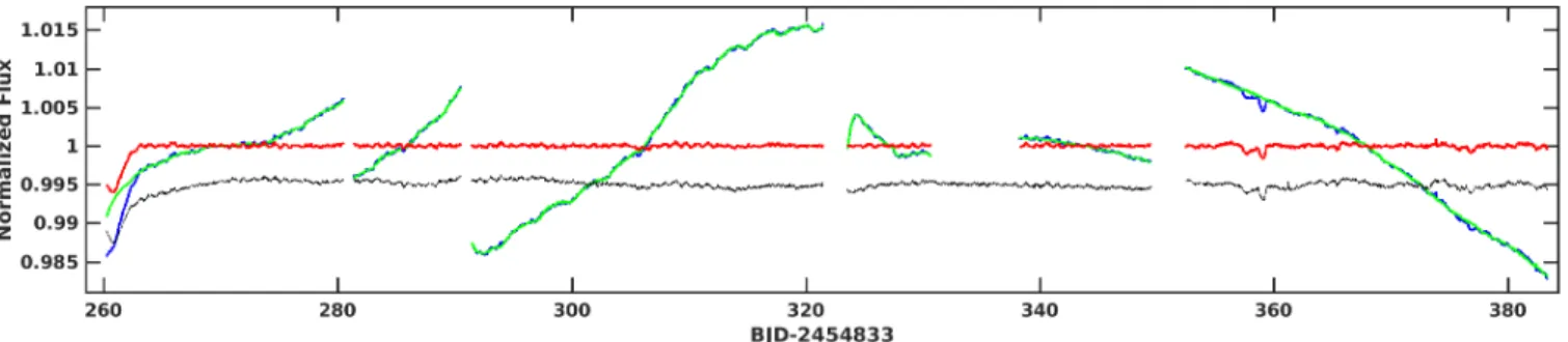
Several examples of the detrending results are shown in Fig.1. We compare these results to the pipeline automatic PDC reduction, which in general presents quarter-long low amplitude variations along the curve and especially around strong dips. With our reduction the continuum is flat, allowing the shallower dips to emerge more evidently than in the PDCSAP data. This shows the positive effect of excluding the measurements of the dips when fitting out the systematics. The full detrended light curve is plotted in Fig.2.
3. Two identical photometric shallow events
Using the light curve obtained in the previous section, we can identify the photometric events that happened during the four years of observation. The observed photometric variations show two different patterns: periodic-like variations and short-time de-creases of star brightness. With a period close to 1 day, the peri-odic modulation corresponds to the 0.88-day signal due to stellar rotation that was already mentioned byBoyajian et al.(2016). Beyond these variations, the stars show significant short-time and sporadic variations, all of which are dips of the star bright-ness below the mean brightbright-ness observed during the quiet period. We screen the entire light curve and identified a total of 22 significant dips. Apart from the strong dips already listed by Boyajian et al.(2016), we found several shallower dips, some of which are also identified byMakarov & Goldin(2016). Table1 summarizes these detections.
Among the detected features, two events show a remark-able similarity in shape, duration, and depth: the events #2 and #13 in Table 1. Hereafter, we label these events as “event A” and “event B”. The light curves of these two events are plotted in Fig.3. In this figure, we superimposed the raw SAPs, fitted CBVs, and corrected SAPs, showing that the two photometric dips are real and not produced by the data analysis procedure.
As indicated in Table1, events A and B were already noticed byMakarov & Goldin(2016) but they were suspected to be due to either the centroid modulation of the point spread function (PSF) during event A, or instrumental jitter (event B). In Sect. 4,
Fig. 1.Example of CBVs fit on light curves with small or no dips. The raw SAP light curve is indicated in blue, the fitted CBVs are indicated in green, and the final detrended SAP light curve is indicated in red. For comparison, we superimposed in black the PDCSAP data with an offset of −0.005 for visual convenience. The green and blue curves overlap most of the time, but it can be seen on some shallow dips (e.g. at BJD-2 454 833= 360) that the fitted CBVs, shown in green, stay at the baseline level during these events.
200 400 600 800 1000 1200 1400 BJD-2454833 0.8 0.85 0.9 0.95 1 Normalized Flux
Fig. 2. Full KIC 8462852 detrended light curve.
Fig. 3.Light curves at the time of the photometric events A (top panel) and B (bottom panel). The curves show the detrended (red) and unde-trended (blue) data sets. The fitted CBVs continuum is plotted with a green line.
we show that these events are of astrophysical origin and are not related to instrumental systematics.
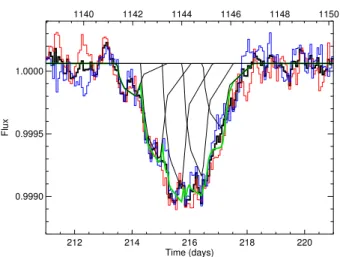
Fitting events A and B together, we derived a time separation between them of∆t = 928.25 ± 0.25 days. The error bars on the flux were scaled to obtain a reduced χ2of 1. Shifting the second
event light curve by –∆t, i.e. on top of the first event light curve, we obtained a strikingly almost perfect superimposition of the two events as shown in Fig.4.
212 214 216 218 220 222 Time (days) 0.9990 0.9995 1.0000 1.0005 Flux 1140 1142 1144 1146 1148 1150
Fig. 4. Two events superimposed with 3-pixel binning. The bottom x-axis shows the time at the first photometric event A (red line). The top x-axis shows the time at the second photometric event B (blue line) with a shift of 928.25 days relative to the bottom axis.
To characterize the similarity of these two photometric events and compare this pair with the 22 detected events, we plotted the depth and duration of each of the events (Fig.5). The depths are measured between the continuum level fixed to 1 and the bottom of the light curve defined as the fifth lowest pixel. The durations are measured by calculating the second mo-ments of the variations, which are then multiplied by 2
√ 2 ln 2 to roughly correspond to the full width at half maximum. While other photometric events show a wide diversity in duration and depth, events A and B are remarkably identical. To emphasize this result, we superimposed the light curves of the photometric events #6 and #9, which are, after the events A and B, the closest
Table 1. List of detected photometric dips in the KIC 8462852 light curve.
Event Epoch Depth Width Comment Previous publications†
(JD-2 454 833) (log10∆F/F) (day)
1 140.7 –2.30 1.70 cometary tail shape (triangular) B2016, MG2016
2/A 215.8 –2.96 1.98 similar to event 13 MG2016: modulation of PSF centroid
3 261.0 –2.23 1.19 cut by a gap B2016, MG2016
4 357.9 –3.03 0.70 cometary tail shape (triangular)
5 359.0 –2.82 0.41 superimposed on event 4 B2016 6 376.6 –3.08 1.25 noisy surrounding MG2016 7 427.1 –3.10 1.78 partly fitted by CBVs B2016, MG2016 8 688.6 –3.18 0.68
series of 4 small dips
9 694.3 –3.03 1.18
10 700.6 –3.32 1.72
11 706.7 –3.37 0.94
12 792.6 –0.90 0.77 very deep event B2016, MG2016
13/B 1144.1 –2.97 1.98 similar to event 2 MG2016: instrumental jitter
14 1206.2 –2.38 2.54 narrow event upon a wide event B2016, MG2016
15 1224.0 –3.02 1.63 shallow event
16 1496.0 –2.60 0.55 cometary tail shape (triangular) B2016
17 1511.4 –2.10 2.24 preceding a much deeper event
18 1519.4 –0.71 1.00 very deep event B2016, MG2016
19 1540.4 –1.75 0.43 deep event B2016, MG2016
20 1542.9 –2.43 0.73 triangular
21 1563.7 –2.60 0.89 cometary tail shape (triangular)
22 1568.2 –1.21 1.03 deep event B2016, MG2016
Notes. Events 2 and 13 are renamed A and B, respectively, in the rest of the paper.(†) MG2016=Makarov & Goldin(2016), Table 1; B2016=
Boyajian et al.(2016), Table 1.
-3.5 -3.0 -2.5 -2.0 -1.5 -1.0 -0.5 Log 10 (Depth) 0.0 0.5 1.0 1.5 2.0 2.5 3.0 Duration (days)
Fig. 5.Depth and duration of the 22 events catalogued in Table1. The events A and B are shown by red and blue symbols, respectively. The events #6 and #9 are shown by green and orange symbols, respectively.
in the depth-duration diagram (Fig. 6). It is clear that, unlike events A and B, these photometric events do not show similar light curve shapes.
The light curve shapes of events A and B can be obtained by fitting a simple four-vertices polygon to each curve. We mea-sured the quantities such as ingress, egress, and centroid timings, slopes of the left and right wings, and transit depth (Table 2). These simple fits quantitatively confirm that the two events are strikingly similar. The average duration of the two events from ingress to egress is measured to be 4.44 ± 0.11 days. The bottom of the light curves are flat with a duration of about 1 day. The two slopes on each side of the flat bottom are straight with compara-ble duration between 1.5 and 2 days. The right wings are steeper
372 374 376 378 380 382 Time (days) 0.9990 0.9995 1.0000 1.0005 Flux 688 690 692 694 696 698 700
Fig. 6.Events #6 and #9 superimposed with 3-pixel binning. The bot-tom x-axis shows the time at the first phobot-tometric event #6 (green line). The top x-axis shows the time at the second photometric event #9 (or-ange line) with a shift of 316.3 days relative to the bottom axis. than the left wings with respective slopes of about 700 ppm/day and −500 ppm/day. The transit depths are similar in both events at about 1010 ± 40 ppm.
If real, these similar events could be the repeated observation of the same periodic phenomenon. After checking for potential reduction artefacts and other systematics in the next section, we discuss interpretations of this repeating event in Sect.5.
4. Possible bias
Makarov & Goldin (2016) argued that some of the small am-plitude features could be of instrumental or background origin.
Table 2. Four-vertices polygon parameters of the fit to the events A and B light curves.
Event A Event B Continuum Ftop− 1 (ppm) 0.9 ± 6.9 1.3 ± 6.5 Left wing slope (10−4day−1) –4.94 ± 0.24 –5.24 ± 0.30 ∆t (day) 2.10 ± 0.09 1.87 ± 0.10 noise (ppm) 123 148 tingress(day) 213.32 ± 0.06 1141.83 ± 0.08 Bottom depth (ppm) 1039 ± 25 978 ± 16 ∆t (day) 1.00 ± 0.07 0.92 ± 0.07 noise (ppm) 123 109 tcentroid(day) 215.93 ± 0.05 1144.15 ± 0.05 Right wing slope (10−4day−1) 7.41 ± 0.28 6.18 ± 0.20 ∆t (day) 1.40 ± 0.04 1.58 ± 0.05 noise (ppm) 100 142 tegress(day) 217.83 ± 0.01 1146.19 ± 0.03
Notes. We used a 4-degree polynomial to fit out the baseline and as-sumed that the bottom of the light curve is flat. Beginning-of-ingress, centroid, and end-of-egress timings are given in days past Kepler initial epoch at MJD 2 454 833.
We thus carefully inspected the pixel tables collected by Kepler around the PSF of the star and used to produce the raw SAP light curve about the epochs of the two events to exclude any instru-mental origin for these events or the possibility of contamination from close background stars.
4.1. Background stars
The closest known stars in the field are Gaia 208190073864563 1744 (at 5.400 with m
G= 18.1), which is referred to as
Gaia-208 in the following, and the infrared sources 2MASS J20061551+4427330 (at 8.900 with m
J= 16.1, mG= 18.9) and
2MASS J20061594+4427365 (at 11.8300 with m
J = 16.4,
mG = 18.7). Their high visual magnitude measured by
Gaia (van Leeuwen et al. 2017) implies a ∆V > 6.4 with KIC 8462852 (mG= 11.7), i.e. a flux ratio <0.3%.
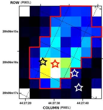
As can be seen in Fig.7, the pixels corresponding to the theoretical location of the two IR sources in the CCD chan-nel are not within the aperture used to calculate the raw light curve. We see that the flux of KIC 8462852 is smeared on an area about 10 × 10 arcsec2 wide. Since the PSF of the two red stars is likely of similar extension, a bit less than half the flux of 2MASS J20061551+4427330 enters the PSF, while there is al-most none for 2MASS J20061594+4427365. Consequently, any flux variation of these stars of order 100% contaminates the flux to a level lower than 0.1%.
However, since the PSF of Gaia-208 almost fully overlaps with the PSF of KIC 8462852, the photometric variations of this polluting star might induce variations in the light curve, but in any case these variations would not be higher than 0.3%.
At this stage, while we are able to exclude contamina-tion from the two IR background stars, contaminacontamina-tion from Gaia-208 cannot be ruled out, although likely to be negligible. In Sect.4.3, we show that no significant and correlated PSF mo-tion of KIC 8462852 is observed during the two events; this ad-vocates for rejecting contamination from any background stars.
Fig. 7.Pixel table of flux around KIC 8462852, collected during quarter # 2 on CCD channel 32. The colours are logarithmically scaled with the flux. The aperture is shown in solid red line. A right ascension and declination grid is superimposed with dotted black lines. The theoret-ical position of KIC 8462852 on the CCD is depicted as a red star; the position of the two faint IR sources 2MASS J20061551+4427330 & 2MASS J20061594+4427365 are indicated by white stars; and Gaia 2081900738645631744 appears as a black star.
4.2. Light curve of closest neighbour KIC 8462934
KIC 8462934 is the closest bright star (about 8900with V ∼ 11.5)
to KIC 8462852 (V = 12) with a recorded light curve in the Keplerdatabase. Applying our previously introduced detrending method, we recovered a detrended light curve using the first 13 CBVs of each quarter/channel, as was applied to light curve of KIC 8462852 (see Sect.2). We found no peculiar behaviour, nei-ther strong nor shallow absorptions similar to what we observed in KIC 8462852. No features were detected in the light curve be-yond a few 10−4in normalized flux. This indicates that the CBVs derived by the Kepler pipeline did not miss any small local vari-ations in, e.g. pixel sensitivity, in the CCD channel. Therefore, events A and B are indeed features from the local pixels in the photometric aperture shown in Fig.7.
4.3. Point spread function motion of KIC 8462852 on CCD pixels
Makarov & Goldin (2016) studied the correlation of the PSF centroid motion and the flux dimming in KIC 8462852. They show that a few features could be artifacts of occultation or in-strumental jitter of background objects.
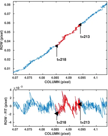
Repeating a similar analysis on the pixel images collected by Keplerat each cadence, such as presented in Fig.7, we derived the centroid motion of the PSF of KIC 8462852 before, during, and after the epoch of each identified event. Apart from an ex-pected slow shift (0.004 pixel day−1) of the location of the star on the CCD channel during the quarter, we observed that the centroid oscillates with a period of about three days and an am-plitude of at most a few 0.001 pixel (Fig.8). This oscillation is likely related to a vibration mode of the instrument. Consistently,
4.07 4.075 4.08 4.085 4.09 4.095 4.1 COLUMN (pixel) 6.01 6.02 6.03 6.04 6.05 6.06 6.07 6.08 ROW (pixel) t=213 t=218 4.07 4.075 4.08 4.085 4.09 4.095 4.1 COLUMN (pixel) -4 -2 0 2 4
ROW - FIT (pixel)
10-3
t=213 t=218
Fig. 8.Top panel: position of the PSF centroid around event A, from epochs 208 to 225 (in blue), and highlighted in red, from ingress (213) to egress (220). Time arrow goes from top right to bottom left. Bottom panel: PSF centroid motion around the 4th degree polynomial fit of the main trend in the top panel. The modulation period is about 3 days. it was found that a few pixels show shallow flux modulations of a few 0.1% in correlation or anti-correlation with the PSF centroid oscillations.
Impressively, these instrumental modulations exactly cancel out. We found no counterpart for these modulations in the raw light curve, demonstrating the excellent quality of the flat-field determination made by Kepler on the aperture. Since the ampli-tude of the three-day modulation is similar to the ampliampli-tude of the two events discussed in this paper, instrumental PSF varia-tions cannot be at their origin. Indeed, in such a case, we would have observed 0.1% deep three-day modulation rather than only single dips.
We have seen in Sect.4.1that the closest background star, Gaia-208, is located at 5.400 from KIC 8462852. This is a bit more than 1 pixel apart, on the aperture (Fig.7). The luminosity variation due to the occultation of a third of Gaia-208 stellar disk would be close to 0.1%, leading to a PSF centroid variation of about 10−3 pixels. We can exclude from Fig.8a PSF centroid
variation of this amplitude during event A between day 213.3 and day 217.8.
Repeating this analysis for event B led to the same conclu-sion. We thus exclude for both events any significant PSF motion correlated with the light curve, eliminating background star pol-lution and instrumental variations as possible origins.
4.4. Local pixel variations
As a final check, we verified the collective variations of the local flux in each pixel around the PSF of KIC 8462852 at different
times between the beginning and end of both events. It clearly appeared that the whole image of the star was fainting during the dimming events, thus confirming that its origin is neither re-lated to background objects occultation nor associated with any instrumental PSF motion.
5. Models
We can try to explain the repeated photometric event observed 928 days apart. The observed variations correspond to a dip in the star brightness by about 0.1%, which lasted for about 4.4 days. In the context of a star that always shows multiple pho-tometric variations in the form of brightness decrease, any other decrease in the star brightness suggests an explanation by the transit of a partially occulting body. With that in mind, the du-ration of the event (∼5 days) is puzzling. With a possible period of 928 days, and assuming 1.4 solar mass for the F3V central star, the corresponding semi-major axis is 2.1 au and the orbital velocity on a circular orbit is 24.4 km s−1. At this transiting ve-locity, the maximum transit time in front of a R∗ = 1.3 R star
is about 10.3 h. Even on a highly eccentric orbit and observed at apoastron, the transit of a body on a 928-day period orbit can-not last longer than 14.6 h. Therefore, the photometric events of 4.4 days can be explained by the transit of an occulting body only if this body is significantly larger in size than the star; in this case, the duration of the transit is related to the size of the object itself.
The main scenario for explaining the other deeper dips in the KIC 8462852 light curve invokes the transit of trains of extrasolar comets (Boyajian et al. 2016; Bodman & Quillen 2016) or planet fragments (Metzger et al. 2017). In fact, the photometric variations observed in KIC 8462852 light curve look like the spectroscopic variations observed in β Pictoris, which can last several days and are interpreted by the tran-sit of exocomets (Ferlet et al. 1987;Lagrange-Henri et al. 1992; Vidal-Madjar et al. 1994;Kiefer et al. 2014a). We explore this scenario in Sect.5.1.
Nevertheless, keeping the idea of a transiting body, we can imagine another possible scenario to explain the repeated pho-tometric events A and B. The straight ingress and egress slopes and the flat bottom of the light curve point towards the possibil-ity that the transiting body can be a single body with a simple shape. Acknowledging that the Hill spheres of a massive planet can extend to several stellar radius in size, the transit of a ring system surrounding a giant planet could explain the observed photometric event A and B, as in the light curve of 1SWASP J140747.93-394542.6 (also named J1407), an old star in the Sco-Cen OB association (Kenworthy & Mamajek 2015); see also Lecavelier Des Etangs et al.(2017) andAizawa et al.(2017) for other case studies of exoplanetary ring systems. This scenario is discussed in Sect.5.2.
5.1. Comets string model
In the exocomets scenario, the duration of the transit event in the light curve implies that several comets passed in front of the star, within an extended string of several million kilometers long. While we do not aim to explore the whole range of possibili-ties to fit the events A and B light curves, we could use some of the exocomet tail transit signatures given, e.g. in the library ofLecavelier Des Etangs(1999), to show that a generic transit model of a few trailing exocomets can easily provide a satisfac-tory fit to the data.
As a reference light curve, we decided to use the light curve labelled “20_F_50_03_p4_00” inLecavelier Des Etangs(1999)
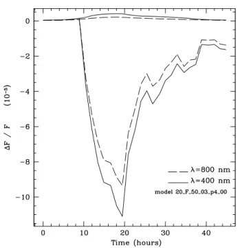
Fig. 9. Modelled exocomet transit light curve from
Lecavelier Des Etangs (1999) for the case “20_F_50_03_p4_00”,
corresponding to an exocomet orbiting an F star with a periastron of 0.3 au, a longitude of periastron of 90◦
, and a production rate of 105kg s−1at 1 au.
and plotted in Fig.9. This plot is obtained through the simulation of cometary tails orbiting an F star with a periastron of 0.3 au, a longitude of periastron of 90◦, and a production rate of 105kg s−1
at 1 au (Lecavelier Des Etangs et al. 1999). It assumes a grain size distribution given by dn(s) = (1 − s0/s)ms−nds, with s0 =
0.05 µm, n= 4.2, m = n(sp− s0)/s0, and peaking at sp= 0.2 µm.
This distribution is derived from observations in solar system comets at less than 0.5 au from the Sun. The physical model used to calculate the photometric transit signatures of exocomet tails is discussed in depth inLecavelier Des Etangs et al.(1999). The choice of the characteristics (the orbit and dust produc-tion rate) of the specific exocomet for the reference light curve is not critical because all the transit light curves show a similar triangular shape. At a fixed distance to the star, the transit depth of an individual light curve is constrained by the dust produc-tion rate, and the duraproduc-tion is mainly related to the longitude of the periastron. The depth of the global light curve resulting from the transit of a string of several exocomets therefore depends on the production rate of each exocomet. However, the duration of the global light curve is not constrained by the duration of each individual transit, but by the spread of the transit time of each exocomet.
To simplify the fit to the data, we approximated the refer-ence light curve of a single comet by a piecewise linear function. Each individual exocomet light curve is defined by two parame-ters: the time of mid-transit, T0, and the maximum occultation
depth, ∆F/F. Exploring the library of Lecavelier Des Etangs (1999), we find that in the range 104–106kg s−1 the maximum
occultation depth is related to the dust production rate, ˙M, by log10M/(1 kg s˙ −1)= 5 + 1.25 × log
10(∆F/F/10−4).
We fitted the average light curve of events A and B with a combination of several individual light curves defined by T0k
and ˙Mk for each comet k of the string. With N comets in the
string, the total number of parameters reach 2N + 1 with two parameters per comet and one for the baseline level (slightly larger than 1). Given the possibly large number of parameters,
212 214 216 218 220 Time (days) 0.9990 0.9995 1.0000 Flux 1140 1142 1144 1146 1148 1150
Fig. 10.Fit to the light curve using a string of 7 exocomets. The light curve of each exocomet is given by the thin black lines. The data of the events A and B are plotted with red and blue thin lines, and the co-addition of the two light curves is given by the thick black line. The best fit is plotted with the thick green line.
we used a Markov-chain Monte Carlo (MCMC) algorithm as a fitting procedure.
The best fit is obtained for seven comets, including the fea-ture at the top of the signafea-ture left wing. It is plotted in Fig.10 with the parameters given in Table 3 and plotted in Fig. 12. The dust production rates obtained for the comets are typical of Hale-Bopp type comets in the solar system, i.e. between 105 and 106kg s−1(Huang et al. 2000).
If we consider that we are actually overfitting stellar vari-ations, we could accept a poorer fit with residuals of the or-der of the mean amplitude of the stellar variations. In this case, five comets are sufficient to fit the average light curve satisfy-ingly. An example of such a fit is shown in Fig.11with the pa-rameters given in Table3and plotted in Fig.12. Here we used a different longitude of periastron of 112.5◦and a different grain
size distribution labelled “50” inLecavelier Des Etangs(1999), peaking at 0.5 µm. This shows that the observations cannot con-strain the properties of the comets and that the model of the comets can easily explain the data without any fine-tuning of parameters. Therefore, the values given in Table3should not be considered as measurements on existing bodies, but as possible values for a generic model of a string of exocomets.
Interestingly, both resulting models are reminiscent of the case of the solar system comet Shoemaker-Levy 9 (SL9). The bottom panel of Fig.12shows the distribution of diameters, D (in log-space), with respect to timing of impact with Jupiter of all 21 fragments of SL9 (Hammel et al. 1995;Chodas & Yeomans 1996;Crawford 1997). Since the dust production rate is propor-tional to the surface of the nucleus (all other things equal), log D of SL9 fragments could be compared to log ˙M of events A and B comets (Fig.12, top-panel). We see that in both cases, the dis-tribution of size (evaporation rate) is mainly flat with decreasing size of the comet nuclei at the head and tail of the fragments string. This tentatively suggests events A and B could be the break-up remnants of a bigger body along its orbit. If the peri-odicity of this transit is confirmed later, non-gravitational effects should be properly modelled to take into account a slow relative drift of the fragments.
212 214 216 218 220 Time (days) 0.9990 0.9995 1.0000 Flux 1140 1142 1144 1146 1148 1150
Fig. 11.Same as Fig.10using a string of 5 exocomets.
Table 3. Best-fit parameters for the models with the transit of 7 or 5 exocomets.
Comet Transit time Dust production rate
T0 M˙ (day) (log kg s−1) 7 comets model 1 213.39 ± 0.11 5.56 ± 0.18 2 214.24 ± 0.07 6.03 ± 0.11 3 214.71 ± 0.11 5.97 ± 0.12 4 215.14 ± 0.06 6.16 ± 0.09 5 215.65 ± 0.05 6.12 ± 0.08 6 216.16 ± 0.06 6.08 ± 0.08 7 216.68 ± 0.12 5.69 ± 0.16 5 comets model 1 213.48 ± 0.13 5.43 ± 0.17 2 214.30 ± 0.05 6.02 ± 0.06 3 215.05 ± 0.05 6.15 ± 0.05 4 215.77 ± 0.05 6.10 ± 0.06 5 216.46 ± 0.08 5.80 ± 0.10
Notes. The error bars correspond to 3σ and were estimated using MCMC. The central transit time, T0, is given for event A; a constant
of 928.25 days must be added for event B.
5.2. Planetary ring model
Here we discuss another possible scenario consisting in the tran-sit of a giant ring system surrounding a planet with a 928-day or-bital period (2.1 au semi-major axis). Indeed, a ring system can be stable within half a Hill-sphere radius of a planet. Around a massive planet the Hill sphere can extend up to several stel-lar radii in size; therefore rings (Kenworthy & Mamajek 2015; Lecavelier Des Etangs et al. 2017; Aizawa et al. 2017) or dust envelopes, such as Fomalhaut b (Kalas et al. 2008), can be large enough that the transit duration can reach up to a few days. For instance, the Hill sphere of Jupiter extends up to 0.34 au (73 R ).
To model this scenario, we take the reference frame linked to the planet and consider that the star transits behind the rings. To simplify the problem, we assumed that the planet moves on a cir-cular orbit at 2.1 au (vtransit = 24.4 km s−1) and that the rings are
seen face-on. We considered two simple models of rings and fit
213 214 215 216 217
Transit Time (days) 5.0 5.2 5.4 5.6 5.8 6.0 6.2 6.4 Log 10
Dust Production Rate (kg/s)
1142 1143 1144 1145 0 1 2 3 4 5 6 7 1 1.5 2 2.5 3 3.5
Impact timing [day]
Log(D/1m)
Fig. 12.Top panel: dust production rates and transit times of the transit-ing bodies for the 7 comet model (black dots; Fig.10) and the 5 comet model (red squares; Fig.11). Bottom panel: Shoemaker-Levy 9 frag-ments diameter vs. epochs of impact with the atmosphere of Jupiter. these models to the data using Levenberg-Marquardt minimiza-tion of χ2:
1. The first model consists in a large circular homogenous, constant opacity, ring with a non-zero impact parameter of the trajectory of the star behind the ring during the transit (Fig.13, left panel). In this case, the signature of the transit is round. The data are best fitted with a ring exterior diame-ter of 8.8 R?, an impact parameter of 8.5 R?and an extinction
τ = 0.0014. Nonetheless, this model does not provide a good fit to the data, which show straight wings and a flat bottom. 2. In the second model, the ring is made of an inner core of
constant opacity for r < Rconstand an external ring with an
extinction decreasing with the distance to the star following ∝r−α for r > Rconst (Fig.13, right panel). As can be seen
in the figure, this model provides a much better fit to the data. Using a zero impact parameter, the best fit is found with an outer radius of 4.86 ± 0.15 R?, an interior core of radius
Rconst = 1.91 ± 0.03 R?with constant extinction τ = (9.9 ±
0.1) × 10−4, and an extinction parameter α= 1.70 ± 0.06.
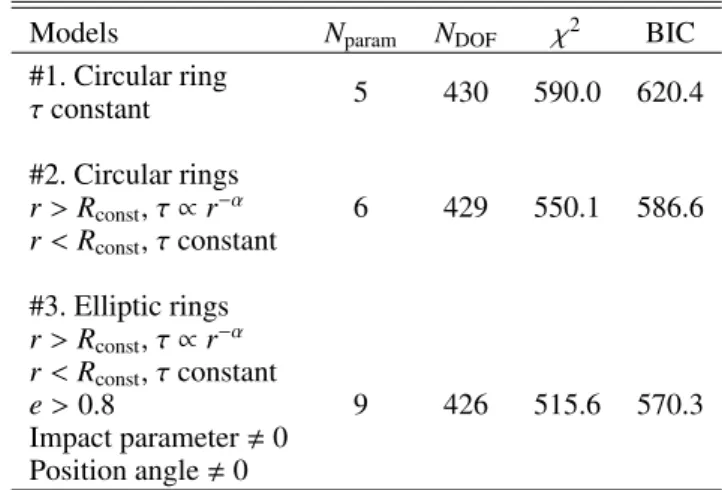
We tried more sophisticated models by introducing elliptical rings, a non-zero impact parameter, and a non-zero position an-gle of the ellipse major-axis with respect to the transit direction (model #3 in Table4). The improvement of the fit is significant but only indicates that the rings as seen from Earth are likely el-liptic (e > 0.8) and not aligned with the transit direction. This is in accordance with the observed asymmetry on the slopes of the left and right wings, as explained in Sect.3. Since the projection
Fig. 13.Fit to the average light curve of events A and B (in red) by the two models of the occultation of KIC 8462852 by a planetary ring, as presented in Sect.5(black curves). Top panel: homogeneous circular ring with a constant opacity and a non-zero impact parameter. Bottom panel: circular ring with a constant opacity in the centre (red area) and a decreasing opacity with distance following a r−αlaw in the external ring (blue area). The impact parameter is fixed to 0. The black circle represents the edge of stellar disk.
of an inclined circle is an ellipse, the eccentric solution corre-sponds to a circular ring system inclined with respect to the plane of the sky at angle θ(= arcsin e) > 53◦.
Interestingly,Ballesteros et al.(2018) recently proposed that the two main dips (D800 and D1500) of KIC 8462852 could be related to a ring planet on a 12-year orbit with trailing trojans at the L5 point. If true, KIC 8462852 might be the first exoplanetary system with two ring planets detected.
6. Observing future events
With the last event on BJD 2 455 977.15 and assuming periodic-ity with P = tB− tA = 928.25 ± 0.25 days, the phenomenon is
expected to repeat itself every tB+ N × P. The occurrence timing
closest to the present date is for N= 2 (event D) with
TD= 2 457 833.65 ± 0.80 (2)
or between 20 March 2017 at 07:55 UT and 21 March 2017 at 23:17 UT.
The beginning-of-ingress and end-of-egress timings were also estimated. Table5summarizes this information.
We planned to observe KIC 8462852 between 19 March and 23 March 2017 in photometry and/or spectroscopy. Un-fortunately, HST and Spitzer were both unable to point at KIC 8462852 on these dates. Current ground-based photometry
Table 4. Table of χ2and BIC of the different ring models proposed in
the text.
Models Nparam NDOF χ2 BIC
#1. Circular ring 5 430 590.0 620.4 τ constant #2. Circular rings 6 429 550.1 586.6 r> Rconst, τ ∝ r−α r< Rconst, τ constant #3. Elliptic rings 9 426 515.6 570.3 r> Rconst, τ ∝ r−α r< Rconst, τ constant e> 0.8 Impact parameter , 0 Position angle , 0
Notes. The value τ is the extinction.
Table 5. Timing and ephemeris of transit events with P= 928.25 days starting from event B at tB = 1144 days past Kepler initial epoch at
MJD 2 454 833.
MJD UT date
Most recent event in the past at tB+ 2 × P (event D)
Tingress 2 457 832.40 ± 0.70 19/03/17 (04:48) → 20/03/17 (14:24) Tcentroid 2 457 833.65 ± 0.80 20/03/17 (07:55) → 21/03/17 (23:17) Tegress 2 457 835.70 ± 0.60 22/03/17 (14:24) → 23/03/17 (19:12) Next event in the future at tB+ 3 × P (event E)
Tingress 2 458 760.65 ± 0.74 03/10/19 (09:30) → 04/10/19 (21:30) Tcentroid 2 458 761.90 ± 0.84 04/10/19 (13:00) → 06/10/19 (06:00) Tegress 2 458 763.95 ± 0.64 06/10/19 (19:00) → 08/10/19 (02:30)
is not sensitive and stable enough to confirm a 0.1% deep tran-sit signature lasting several days. We attempted ground-based spectroscopy since in case of exocomet transit, variable Na I or Ca II features could be expected in the KIC 8462852 spec-trum (Kiefer et al. 2014a,b;Beust et al. 1990;Ferlet et al. 1987). We therefore planned observations of the star with the SOPHIE spectrograph installed on the 1.93 m telescope of Observatoire de Hautes-Provence (Perruchot et al. 2008;Bouchy et al. 2009) between 15 and 26 March 2017.
Unfortunately, bad weather conditions prevented us from ob-serving KIC 8462852 after the 19 March 2017. We were able to collect good quality spectra of KIC 8462852 on 15, 16, 17, and 19 March between 03:30 and 03:45 UT. The median Na I spec-trum of KIC 8462852 observed with SOPHIE between these four dates is plotted in Fig.14. On the right-hand side of the stellar Na I doublet lines, we detected an emission feature, which is also observed in the simultaneous sky-background spectrum obtained through the second aperture of the spectrograph (fiber B). It is identified as geocoronal emission from atmosphere of the Earth. We subtracted this feature from all Na I spectra by fitting out the
Fig. 14.Na I spectra of KIC 8462852. In blue, the average of the spectra collected through fiber A of the SOPHIE spectrograph, on the 15, 16, 17 and 19 March 2017. In grey, the average sky-background spectrum taken simultaneously with each star’s spectrum on fiber B. The emission line seen on fiber A and B is clearly identified as geocoronal sodium emission. The double peak feature on the left of the telluric emission is most probably of interstellar absorption origin, since no counterpart is observed in the Ca II spectrum at the star radial velocity (see Fig.16).
5885 5890 5895 5900 Wavelength [A] -3 -2.5 -2 -1.5 -1 -0.5 0 0.5 1 Normalized Flux 16/04/2017 - 3:26:42 UT 17/04/2017 - 3:34:37 UT 19/04/2017 - 3:45:12 UT 15/04/2017 - 3:30:58 UT
Fig. 15. Comparison of the Na I spectra of KIC 8462852 ordinated by increasing dates from top to bottom. The sky spectrum obtained si-multaneously in fiber B has been fitted out of the original spectra (see Fig.14).
sky spectrum. As can be seen in Fig.15, the resulting Na I spec-trum is totally quiet throughout the four days. It only presents a stable double peak absorption line, which is most likely of interstellar origin, since no counterpart is observed in the Ca II spectrum at the star radial velocity (Fig.16). Similarly the Ca II doublet spectrum of KIC 8462852 does not present any variable features between 15−19 March.
Nevertheless, the predicted time of ingress is just after the observation dates. At the top of the signature left wing is 19 March at 03:45 (UT) before the predicted timing of ingress (19 March 04:48 UT). Therefore, the absence of observed fea-tures cannot exclude that significant absorption occurred in the KIC 8462852 spectrum during the transit. The observed spectra could neither confirm nor refute the periodicity of these transit events.
Assuming periodicity, the next event is predicted to occur between 3−8 October 2019 with ingress, centroid, and egress timings given in Table5. New observations of KIC 8462852 be-tween 3−8 October 2019 in both photometry and spectroscopy, with Spitzer, Cheops, HST, JWST, and ground-based spectro-scopes, are strongly encouraged. They should allow confirma-tion or refutaconfirma-tion of the periodicity in the observed photometric event. 3920 3940 3960 3980 4000 Wavelength [A] -3 -2 -1 0 1 2 Normalized Flux 19/04/2017 - 3:45:12 UT 17/04/2017 - 3:34:37 UT 16/04/2017 - 3:26:42 UT 15/04/2017 - 3:30:58 UT
Fig. 16. Comparison of the Ca II spectra of KIC 8462852 ordinated by increasing dates from top to bottom, with 3-pixel binning. As can be seen, there are no spectral signatures of transient phenomenon in these spectra.
7. Conclusions
After a careful detrending of the Kepler light curve of the pe-culiar star KIC 8462852, we identified among 22 signatures, two strickingly similar shallow absorptions with a separation of 928.25 days (event A and B). These two events presented 0.1% deep stellar flux variations with duration of 4.4 days, which is consistent with the transit of a single or a few objects with a 928-day orbital period.
We thoroughly verified the different possible sources of sys-tematics that could have produced the transit-like signatures of event A and B. We conclude that these two events are certainly of astrophysical origin and occurred in the system of KIC 8462852. We found that two scenarios could well reproduce the transit light curve of events A and B. They consist in the occultation of the star by two kinds of objects:
1. A string of a half dozen exocomets orbiting at a distance &0.3 au with evaporation rates similar to comet Hale-Bopp and scattered along their common orbit much like the 1994 Shoemaker-Levy 9 fragments.
2. An extended ring system surrounding a planet orbiting at 2.1 au from the star and composed of a constant opacity inte-rior ring and an exteinte-rior ring with decreasing opacity towards larger radius.
It should be mentioned that the main argument against the exo-comet scenario for KIC 8462852 dimming events is the absence of any detectable IR excess. This is an important problem that will always lead to risky comparison with other emblematic ex-ocomet hosts such as β Pic. These stars are all young (<100 Myr) with strong Vega-like excess and thus massive debris disk. The age of KIC 8462852 (1 Gyr) would explain well the lack of IR excess, yet how the vaporization of the remaining small bodies would fit below the detection level remains to be explained. In fact,Boyajian et al.(2016) showed that dust clouds of the mass of a fully vaporized Hale-Bopp comet, as needed to explain the strongest dips of the KIC 8462852 light curve, are not expected to produce visible IR emission as long as the distance of the clouds is greater than 0.2 au. This happens to be the case in the exocomets string model proposed here.
This is the first strong evidence for a periodic signal com-ing from KIC 8462852. All the other dimmcom-ings present irregu-lar behaviour with apparently uncorrelated timings. If periodic, our discovery opens a gate for the in-depth characterization of
a collection of objects present around this star. Assuming pe-riodicity, we predict that the next event to happen will occur between 3−8 October 2019. The observation of KIC 8462852 at these dates will confirm or deny the 928.25-day period, and hopefully will allow us to discriminate between the two scenar-ios proposed in this paper.
Acknowledgements. We thank the anonymous referee for a careful reading of our manuscript and insightful comments and suggestions. This work has been supported by the Centre National des Etudes Spatiales (CNES). We acknowl-edge the support of the French Agence Nationale de la Recherche (ANR), under programme ANR-12-BS05-0012 “Exo-Atmos”. V.B. acknowledges the financial support of the Swiss National Science Foundation. This paper includes data col-lected by the Kepler NASA mission and with the SOPHIE spectrograph on the 1.93 m telescope at Observatoire de Haute-Provence (CNRS). Funding for the Keplermission is provided by the NASA Science Mission directorate.
References
Abeysekara, A. U., Archambault, S., Archer, A., et al. 2016,ApJ, 818, L33
Aizawa, M., Uehara, S., Masuda, K., Kawahara, H., & Suto, Y. 2017,AJ, 153, 193
Ballesteros, F. J., Arnalte-Mur, P., Fernandez-Soto, A., & Martinez, V. J. 2018,
MNRAS, 473, L21
Beust, H., Vidal-Madjar, A., Ferlet, R., & Lagrange-Henri, A. M. 1990,A&A, 236, 202
Bodman, E. H. L., & Quillen, A. 2016,ApJ, 819, L34
Borucki, W. J., Koch, D., Basri, G., et al. 2010,Science, 327, 977
Bouchy, F., Hébrard, G., Udry, S., et al. 2009,A&A, 505, 853
Boyajian, T. S., LaCourse, D. M., Rappaport, S. A., et al. 2016,MNRAS, 457, 3988
Chodas, P. W., & Yeomans, D. K. 1996, The Collision of Comet Shoemaker-Levy 9 and Jupiter,IAU Colloq., 156, 1
Crawford, D. A. 1997,Ann. N. Y. Acad. Sci., 822, 155
Ferlet, R., Vidal-Madjar, A., & Hobbs, L. M. 1987,A&A, 185, 267
Hammel, H. B., Beebe, R. F., Ingersoll, A. P., et al. 1995,Science, 267, 1288
Harp, G. R., Richards, J., Shostak, S., et al. 2016,ApJ, 825, 155
Hippke, M., & Angerhausen, D. 2016, ArXiv e-prints [arXiv:1609.05492] Hippke, M., Angerhausen, D., Lund, M. B., Pepper, J., & Stassun, K. G. 2016,
ApJ, 825, 73
Hippke, M., Kroll, P., Matthai, F., et al. 2017,ApJ, 837, 85
Huang, K., Hu, J., & Zhou, H. 2000, Proc. Observations and Physical Studies of Comet Hale-Bopp and Other Comets, eds. Z. Junliang & W. Ningshan (Shanghai: Ke Xue Ji Sju Chu Ban She), 44
Kalas, P., Graham, J. R., Chiang, E., et al. 2008,Science, 322, 1345
Kenworthy, M. A., & Mamajek, E. E. 2015,ApJ, 800, 126
Kiefer, F., Lecavelier des Etangs, A., Boissier, J., et al. 2014a,Nature, 514, 462
Kiefer, F., Lecavelier des Etangs, A., Augereau, J.-C., et al. 2014b,A&A, 561, L10
Kinemuchi, K., Barclay, T., Fanelli, M., et al. 2012,PASP, 124, 963
Lagrange-Henri, A. M., Beust, H., Ferlet, R., Vidal-Madjar, A., & Hobbs, L. M. 1990,A&A, 227, L13
Lagrange-Henri, A. M., Gosset, E., Beust, H., Ferlet, R., & Vidal-Madjar, A. 1992,A&A, 264, 637
Lecavelier Des Etangs, A. 1999,A&AS, 140, 15
Lecavelier Des Etangs, A., Vidal-Madjar, A., & Ferlet, R. 1999,A&A, 343, 916
Lecavelier Des Etangs, A., Hébrard, G., Blandin, S., et al. 2017,A&A, 603, A115
Lisse, C. M., Sitko, M. L., & Marengo, M. 2015,ApJ, 815, L27
Lund, M. B., Pepper, J., Stassun, K. G., Hippke, M., & Angerhausen, D. 2016, ApJ, submitted [arXiv:1605.02760]
Makarov, V. V., & Goldin, A. 2016,ApJ, 833, 78
Marengo, M., Hulsebus, A., & Willis, S. 2015,ApJ, 814, L15
Metzger, B. D., Shen, K. J., & Stone, N. C. 2017,MNRAS, 468, 4399
Miles, B. E., Roberge, A., & Welsh, B. 2016,ApJ, 824, 126
Montet, B. T., & Simon, J. D. 2016,ApJ, 830, L39
Montgomery, S. L., & Welsh, B. Y. 2012,PASP, 124, 1042
Neslušan, L., & Budaj, J. 2017,A&A, 600, A86
Perruchot, S., Kohler, D., Bouchy, F., et al. 2008,Proc. SPIE, 7014, 70140J
Schaefer, B. E. 2016,ApJ, 822, L34
Schuetz, M., Vakoch, D. A., Shostak, S., & Richards, J. 2016,ApJ, 825, L5
Smith, J. C., Stumpe, M. C., Van Cleve, J. E., et al. 2012,PASP, 124, 1000
Thompson, M. A., Scicluna, P., Kemper, F., et al. 2016,MNRAS, 458, L39
van Leeuwen, F., Evans, D. W., De Angeli, F., et al. 2017,A&A, 599, A32
Vidal-Madjar, A., Lagrange-Henri, A.-M., Feldman, P. D., et al. 1994,A&A, 290, 245