HAL Id: hal-00510808
https://hal.archives-ouvertes.fr/hal-00510808
Submitted on 18 Feb 2016
HAL is a multi-disciplinary open access
archive for the deposit and dissemination of
sci-entific research documents, whether they are
pub-lished or not. The documents may come from
teaching and research institutions in France or
abroad, or from public or private research centers.
L’archive ouverte pluridisciplinaire HAL, est
destinée au dépôt et à la diffusion de documents
scientifiques de niveau recherche, publiés ou non,
émanant des établissements d’enseignement et de
recherche français ou étrangers, des laboratoires
publics ou privés.
the DEMETER satellite during the 29 March 2006 solar
eclipse
Xiaoni Wang, Jean-Jacques Berthelier, J. P. Lebreton
To cite this version:
Xiaoni Wang, Jean-Jacques Berthelier, J. P. Lebreton. Ionosphere variations at 700 km altitude
observed by the DEMETER satellite during the 29 March 2006 solar eclipse.
Journal of
Geo-physical Research Space Physics, American GeoGeo-physical Union/Wiley, 2010, 115 (A11), pp.A11312.
�10.1029/2010JA015497�. �hal-00510808�
Ionosphere variations at 700 km altitude observed
by the DEMETER satellite during the 29 March 2006
solar eclipse
X. Wang,
1J. J. Berthelier,
1and J. P. Lebreton
2Received 24 March 2010; revised 3 June 2010; accepted 26 July 2010; published 12 November 2010.
[1]
We present an experimental and modeling study of the effects of the 29 March 2006
solar eclipse in the topside ionosphere. Measurements of the densities and temperatures
of the thermal electrons and ions were provided by instruments aboard the Centre National
d’Etudes Spatiales microsatellite DEMETER, which flew over Europe and Africa near
the time of maximum solar obscuration. Data from several orbits, either on the same
day or on days encompassing the eclipse day, were available to determine a reference state
of the ionosphere along the orbit in absence of eclipse. The comparison between this
latter and the actual observations along the eclipse orbit reveal a clear thermal effect with
a fast drop of about 200 K of the electron and ion temperatures that follows the
variations of the solar UV flux in the F region of the ionosphere conjugate to the
satellite position. The plasma density decreases by about 30% but with a significant delay
and is better correlated with the solar UV flux averaged over the previous 1 to 2 h in the
conjugate F region. This delayed and prolonged decrease of density induces an increase
of the electron temperature to be higher than the reference ionosphere. We have also
performed a modeling of the ionosphere using the SAMI2 code, after having introduced
adequate modifications to reproduce fairly realistic eclipse conditions. Applied to the
DEMETER conditions of observation, the model reproduces the observations very well.
This work shows that the plasma temperature responds very quickly along the magnetic
field lines to the variations of the energy available from the photoelectrons while the
plasma density variations are controlled by more complex and slower transport processes.
Citation: Wang, X., J. J. Berthelier, and J. P. Lebreton (2010), Ionosphere variations at 700 km altitude observed by the DEMETER satellite during the 29 March 2006 solar eclipse, J. Geophys. Res., 115, A11312, doi:10.1029/2010JA015497.
1.
Introduction
[2] Solar eclipses have always been of particular interest
to ionospheric researchers since they offer an opportunity to study the response of the ionosphere to a known variation of the solar radiation. In early days it was anticipated that the variations of the ionosphere would provide useful informa-tion on the photochemical processes that control its produc-tion and dynamics [e.g., Anastassiades, 1970], and a large number of experimental and modeling studies have been undertaken during the last decades [Evans, 1965; Roble et al., 1986; Cheng et al., 1992; Boitman et al., 1999; Yeh et al., 1997; Chen et al., 1999; MacPherson et al., 2000; Bamford, 2001]. Although a decrease of the electron density in the bot-tomside ionosphere, up to the peak of the F layer, and of the Total Electron Content (TEC) are regularly observed features, these studies have shown that ionospheric effects of solar eclipses are far more complex than what can be expected
from the simple decrease of the ion and electron production in the shadowed regions. This is true even in the midlatitude and low‐latitude F2 layer [Risbeth, 2000], where the time
variations of the ionospheric plasma reflect a number of intri-cate processes that couple in a complex way photochemis-try, transport, and diffusion along magnetic field lines and, possibly, neutral atmosphere disturbances triggered by its fast cooling along the path of the Moon shadow. This sit-uation has resulted in significantly different and even con-tradictory observations for various eclipses that are often addressing puzzling questions.
[3] While most observations have been conducted on the
bottomside ionosphere using ground‐based measurements of the electron density profiles by ionospheric sounders and more recently TEC determinations from GPS receivers, a number of recent studies have addressed the effects of solar eclipses at higher altitudes. MacPherson et al. [2000] studied the eclipse of 26 February 1998 using observations from the Arecibo radar, and Tomás et al. [2007] reported observations from the CHAMP satellite during the eclipse of 8 April 2005. In this paper we present results obtained during the 29 March 2006 solar eclipse in the upper F region at middle and low latitude on the basis of plasma measurements performed by the Centre National d’Etudes Spatiales (CNES) DEMETER
1
LATMOS, UVSQ, UPMC, CNRS, Saint‐Maur, France.
2Research and Scientific Support Department, ESTEC, ESA, Noordwijk,
Netherlands.
Copyright 2010 by the American Geophysical Union. 0148‐0227/10/2010JA015497
JOURNAL OF GEOPHYSICAL RESEARCH, VOL. 115, A11312,doi:10.1029/2010JA015497, 2010
microsatellite and outputs from a modeling study of the ion-osphere using the SAMI2 code [Huba et al., 2000; 2002]. DEMETER data were available during the “eclipse orbit” with a ground track very close to the location of maximum eclipse in both distance and time. Because of the nearly con-tinuous operation of the satellite at latitudes less than∼65°, a large number of orbits encompassing the eclipse orbit were available to determine a“reference ionosphere” reflecting the normal state of the ionosphere without eclipse. In section 2 we describe the conditions of the 29 March 2006 solar eclipse, and in section 3 we describe the DEMETER observations. A good knowledge of the reference ionosphere is necessary to quantify with enough accuracy the disturbances induced by the eclipse. Determining this reference ionosphere appears, from our own and previous works, as a key and often dif-ficult question, which is discussed in detail in section 4. The SAMI2 model is introduced in section 5, with two configura-tions, to simulate the reference and the eclipse ionospheres, respectively. In section 6 we compare and discuss the simu-lation results and the DEMETER observations and conclude with an interpretation of the physical processes that control the ionosphere variations during a solar eclipse.
2.
Solar Eclipse of 29 March 2006
[4] On 29 March 2006 a total annular solar eclipse occurred,
starting from the sunrise terminator over Brazil at 0836 UT and extending across the Atlantic, Africa, and central Asia where it ended at sunset in Mongolia at 1148 UT. The instant of greatest eclipse occurred at 1011:18 UT over central Africa
at 16.44°E longitude and 23.09°N latitude. In the Northern Hemisphere, the region of partial eclipse extended over a broad region over Europe and central Asia. In Figure 1, reproduced from “Total Solar Eclipse of 2006 March 29” (http://eclipse.gsfc.nasa.gov/SEmono/TSE2006/TSE2006. html), the path of total eclipse and the contour lines of con-stant solar obscuration in the partial eclipse regions are drawn. The solar obscuration is defined as the percentage of the solar disk obscured by the Moon and depends on the time, longitude, latitude, and altitude of the point of observation. The eclipse is displayed for an observer on the Earth’s surface. As seen in Figure 1, the zone of partial eclipse with a significant solar obscuration of >20% extended as high as 60° in latitude in the Northern Hemisphere at the time of maximum total eclipse over Africa.
[5] Three successive dayside half orbits of DEMETER
(referred by orbit number_0 in the text) are also shown in Figure 1. The first (9253_0) and third (9255_0) half orbits occur before and after the eclipse, respectively, and are dis-placed by about 26° in longitude East and West, respectively, from the eclipse orbit. During the second orbit (9254_0), DEMETER itself crossed the Moon shadow and, for a signif-icant part of the satellite path, the northern conjugate F region ionosphere encountered variable eclipse conditions up to a maximum of 50% solar obscuration. The satellite track on the Earth’s surface crossed the total eclipse path at ∼1019:56 UT at 0.72°E and 6.46°N, only∼8 min after the time of maxi-mum eclipse that occurred at 1011:18 UT at 16.44°E and 23.09°N. Data from a number of other DEMETER orbits in the same longitudinal sector are available over a period of Figure 1. Trace of the solar eclipse on the Earth’s surface and DEMETER orbits. Orbit 9254_0 crosses
the eclipse path, orbit 9253_0 is before the eclipse, and orbit 9255_0 is after the eclipse. The contour lines of 100%, 50%, and 20% solar obscuration are shown with green dots, and the location of the greatest eclipse is represented with a red star.
±20 days around 29 March: in particular, two orbits on 28 and 30 March with descending nodes only∼6° from the descending node of the eclipse orbit.
3.
DEMETER Observations
[6] DEMETER was launched on 30 June 2004 on a nearly
Sun‐synchronous orbit, at ∼715 km altitude with 98° incli-nation and a descending node at∼1030 LT. The main objec-tive of the mission is to search for possible disturbances of the ionospheric plasma and plasma waves that could be associated with seismic activity. To this aim, DEMETER is equipped with a fairly complete scientific payload with two instruments dedicated to thermal plasma measurements. IAP, the thermal ion analyzer [Berthelier et al., 2006], provides the density and temperature of the major ionospheric ions O+, H+, and He+, and ISL, a Langmuir probe [Lebreton et al., 2006], provides the electron density and temperature. During standard periods of observations, the scientific payload oper-ates nearly continuously at geographic latitudes less than∼65°.
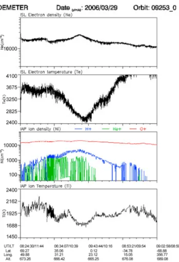
[7] Shown in Figure 2 are the DEMETER measurements
in the daytime half orbit 9253_0. This orbit is preceding the 9254_0 eclipse daytime half orbit by the DEMETER orbital period of∼1.6 h and, therefore, not subject to solar eclipse. The corresponding data are displayed as a typical example of the orbit profile of the topside ionosphere in the African sector. The major ion is O+with a maximum of∼20% H+at low latitudes. Larger plasma densities are observed near the magnetic equator, associated with a lower electron temper-ature. This is consistent with the anticorrelation between electron density and temperature usually observed at mid-latitude because of the heating of a larger number of thermal electrons by a constant photoelectron flux. The absolute accu-racy of the measured ion density is better than∼15%, and its variations are known to be better than∼2%. For ion tempera-tures in the range of 1300 K to 2000 K observed during the eclipse orbit, the absolute accuracy is better than ∼150 K, and its variations are known to be better than∼50 K. The absolute error on the electron density provided by ISL is about 20% to 25%, with errors on their variations better than ∼5%. Measured electron temperature appears to be signifi-cantly larger (by a few hundred degrees kelvin) than that from an empirical ionospheric model such as IRI, an effect attributed to an accidental contamination during launch; however, the errors on their variations are less than∼100 K. DEMETER data are usually displayed as a function of time (UT/LT) with indication of geographic longitude and lati-tude. However, the SAMI2 code, with which we performed the ionosphere modeling, uses a coordinate system based on the Earth’s eccentric magnetic dipole. Therefore, for every position along the orbit, the geographic coordinates are transformed into eccentric magnetic latitude and longitude using the computational method adopted in SAMI2 and described by Huba et al. [2000]. (For the sake of simplicity, the term magnetic will be omitted in the following.) Starting with Figure 3, the four ionospheric parameters, Ne(electron
density), Te(electron temperature), Ni(density of the major
ion species O+), and ion temperature Ti, will thus be
dis-played as a function of eccentric latitudes to ease the direct comparisons between DEMETER data and the SAMI2 results. Because of the high inclination of the DEMETER orbit, the variations of the ionospheric parameters along the orbit mainly depend on the eccentric latitude.
4.
Reference Ionosphere and Eclipse
‐Induced
Disturbances
[8] In order to determine the ionospheric disturbances
induced by the eclipse along the orbit of DEMETER, one has to define a reference ionosphere, i.e., for each ionospheric parameter a baseline that should represent its variation along the eclipse orbit in the absence of solar obscuration. The accurate determination of this reference ionosphere has proved to be difficult in many of the previous works [e.g., Cheng et al., 1992; Huang et al., 1999] because of the lack of suf-ficient observations and, more importantly, because of the large day‐to‐day ionospheric variability [Forbes et al., 2000]. We have thus devoted careful attention to this question.
[9] At the middle and low latitudes, the state of the
ion-osphere depends on several factors, mainly (1) the season; (2) the local time; (3) the solar flux (represented by the F10.7
Figure 2. Orbit profile of ionospheric parameters provided by DEMETER along the day time half orbit 9253 (without eclipse) on 29 March 2006. These data show the usual aver-age state of the ionosphere observed by DEMETER in the African sector at springtime. Coordinates along the horizon-tal axis are UT/LT time, geographic longitude and latitude, and altitude.
WANG ET AL.: IONOSPHERE IN ECLIPSE A11312
A11312
index); (4) the longitude; and (5) two physical parameters, the convection electric field and thermospheric winds that control the dynamics of the plasma in the ionosphere and the plasmasphere.
[10] The convection electric field and thermospheric winds
display large‐scale variations in latitude and local time that mainly depend on auroral activity (represented by the 3 h ap or 3 h Kp index), superimposed with irregular variations responsible for the ionospheric variability. The coupling of auroral phenomena with plasmaspheric electric fields and thermospheric winds is a complicated problem, not well understood so far and beyond the scope of this paper. The influence of auroral activity on the midlatitude ionosphere and plasmasphere depends on the intensity and history of
the auroral events. Strong plasmasphere disturbances are observed following magnetic storms, and the recovery may last many days. However, for the low‐level geomagnetic activity observed on 29 March and 28 March (average ap∼5 and average Kp over the previous 3 days <2), the effects of auroral activity on the midlatitude ionosphere must be low and should not be extended over more than∼12 to 24 h. To build an accurate reference ionosphere, we have thus selected orbits with an instantaneous ap index and a sum of the eight previous ap indices (noted as“ap Sum D1” in Table 1) that are as close as possible to those of the eclipse orbit.
[11] The presence of the South Atlantic anomaly (SAA)
∼30° west of the eclipse orbit and the resulting interaction of quasi‐trapped energetic electrons with the upper atmosphere Figure 3. The DEMETER baselines and observations of the electron and O+densities and of the
elec-tron and ion temperatures during the eclipse orbit (9254_0). The baselines are determined using method I, i.e., the two orbits on 28 and 30 March which cross the equator at a longitude within <5° of that of the eclipse orbit. The color bar represents the period when the ionosphere F region at 250 km conjugate to the satellite position experiences a solar obscuration larger than 20%.
result in noticeable and variable disturbances in the iono-sphere [e.g., Sauvaud et al., 2006]. Since these effects extend significantly eastward from the SAA, using data from orbits more than ∼10° west of the eclipse orbit would likely be a source of inaccuracy in determining the reference ionosphere.
[12] The reference ionosphere can be obtained using three
approaches with their own advantages and drawbacks. The first approach (labeled method I) uses the“same orbits,” i.e., the two orbits 9239_0 (28 March) and 9269_0 (30 March) with descending nodes within≤5° of the eclipse orbit. This has the advantage of making all the variations associated with factors (1), (2), and (4) negligible. In addition the F10.7
index does not vary by more than two units around its mean value between 28 March and 30 March, and the ap Sum D1 in these two orbits are identical to that of the eclipse orbit (see Table 1), and the average Kp over the previous 3 days is <2. Thus, the possible effects of factors (3) and (5) are minimized.
[13] For the sake of completeness, we have also
consid-ered two other approaches, labeled methods II and III, respectively. Method II uses the “same day” orbits, i.e., orbits 9253_0 and 9255_0 in Figure 1. This choice well satisfies the conditions on factors (1), (2), (3), and (5) but not (4) and may thus be impeded by the effect of longitu-dinal variations in the vicinity of the SAA. Method III uses an average over a larger number of orbits in an attempt to lessen the effect of the natural ionospheric variability by averaging over a (hopefully) homogeneous set of random instantaneous conditions. The selected orbits were chosen within a longitude range of maximum 20° east and 15° west of the eclipse orbit to reduce the effects of the SAA. To get a sufficient number of orbits with not too different magnetic activity and solar F10.7 indices, we have been obliged to
extend the selection over a period ±20 days from the eclipse day, which provides a total of 11 orbits, shown in Table 1. Method III should bring some statistical improvement with respect to the first two methods but, using data over an extended period and with more variable auroral activity, certainly prevents reproducing the actual instantaneous conditions of the ionosphere on the eclipse day. In our study we have found that method II and method III offer less reliable references, and by far the most reliable one is method I. The results from method I have thus been used in this study.
[14] The data from each selected orbit of method I are
processed as those of the eclipse orbit, i.e., the eccentric latitude and longitude are computed for satellite positions every ∼2 min and the data are organized as a function of eccentric latitude. The first and last two points are chosen with no (or <10%) solar obscuration, and the reference and eclipse ionospheric parameters should be practically equal at these positions. The mean and standard deviation (shown as error bars in Figure 3) are calculated for each eccentric latitude. Since there are only two data values, the error bar has been represented by the difference between the two values. The baselines for Ne, Te, Ni, Ti estimated are
dis-played in Figure 3, and the observations from the eclipse orbit (9254_0) are also plotted in order to show the varia-tions induced by the eclipse. A color bar is added to indicate the part of the eclipse orbit when the solar obscuration in the conjugate ionosphere is larger than 20%. This part of orbit will be referred as“eclipse zone” in the following.
[15] In Figure 3 (from method I), the baseline electron
temperature (solid blue line) appears to be consistently higher by∼130 K than the eclipse curve (solid red line) on the first and last two points, although no difference should be expected because the conjugate ionospheres are out of the eclipse zone. This gives an estimate of the error made in determining the baseline mainly due to the ionosphere vari-ability and to measurement inaccuracies. An opposite situa-tion is observed on the ion temperature with the baseline about 80 K lower. To take these observations into account we have drawn“corrected baselines” shown as dashed blue lines that are expected to better represent the reference ion-osphere. As far as the electron density and O+ density are concerned, the differences between the baselines and the eclipse observations at the beginning and end of the latitude range are less marked. From a comparison at latitudes >25° South, the Nebaseline may be∼5% too low, but no difference
is observed at the highest northern latitude. A similar ∼5% difference is observed for the Nibaseline at both ends of the
latitude range. This situation does not warrant any improve-ment of the baseline.
5.
Numerical Simulation of Eclipse Effects
[16] In order to help in the interpretation of the
DEME-TER observations, we have performed a numerical model-ing of the ionosphere durmodel-ing the eclipse usmodel-ing the SAMI2 code. SAMI2 is an ionosphere‐plasmasphere simulation code that has been developed at the Naval Research Laboratory (NRL) [Huba et al., 2000] to model the plasma production and transport in any geomagnetic plane. The code uses an eccentric dipole approximation for the Earth’s magnetic field, and one of its main advantages is to set the boundary of the computing domain at 85 km altitude where photo-chemical equilibrium conditions can be safely assumed. In our simulation, the apex of the magnetic field line defining the high‐latitude boundary of the computation plane is at 8000 km altitude, and there are 100 magnetic field tubes with 150 grid points along each tube. The main limitation of SAMI2 is, of course, to be restricted to a geomagnetic plane and thus not to take into account zonal plasma transport. SAMI2 considers seven ions, H+, He+, N+, O+, N2+, NO+,
and O2+, and thermal electrons and solves the continuity and
momentum equations for all species. Thermal balance
equa-Table 1. Selected DEMETER Orbits Used to Determine the Reference Ionosphere With the Corresponding Solar F10.7Index and ap Magnetic Activity Index
Selection
Approach Orbit Number Date ap Sum D1 F10.7
1 9239 and 9269 28 Mar 2006, 30 Mar 2006 35 81 2 9253 and 9255 29 Mar 2006 35 81.5 3 8901 and 8902 5 Mar 2006 13 73 3 8945 and 8946 8 Mar 2006 38 71.3 3 9078 17 Mar 2006 37 71.3 3 9181 24 Mar 2006 22 75.4 3 9210 26 Mar 2006 25 73.3 3 9298 1 Apr 2006 27 86.9 3 9459 12 Apr 2006 21 81.6 3 9562 and 9563 19 Apr 2006 24 76.5
WANG ET AL.: IONOSPHERE IN ECLIPSE A11312
A11312
tions are solved for the three major ionospheric species (H+, He+, and O+) and for electrons. The neutral atmo-sphere is specified by the empirical codes NRLMSISE00 and HWM93. Two parameters control the plasma trans-port: the zonal component of the convection electric field and the meridian component of the thermospheric winds, both being represented by parameterized empirical models. Similarly, the energy transfer from the photoelectrons to the thermal electrons is simulated through an adjustable param-eter cqe in the range from 0.3 to 0.8. By comparing DEME-TER data on orbits close to the eclipse orbit and the SAMI2 results obtained using various models of the electric fields and thermospheric winds and cqe values, we found that the most appropriate configuration for the period of interest is obtained with the Fejer/Scherliess electric field empirical model [Scherliess and Fejer, 1999], the neutral wind model used by Huba et al. [2002] with an amplitude reduced to 80% of its full value and a cqe value of 0.6.
[17] SAMI2 uses the EUVAC solar EUV flux model to
calculate photoionization rates [Richards et al., 1994]. To represent the variation of the solar flux at any position and time during the eclipse, we have introduced in SAMI2 a solar obscuration function that depends on time, latitude, longitude, and altitude using a code developed by Pierre Rocher at Institut de Mecanique Celeste et de Calcul des Ephemerides, Paris Observatory. This code computes at any position the relative area of the solar disk that is masked by the Moon, and the solar UV flux impinging on the ion-osphere is taken proportional to the nonobscured area of the solar disk. This assumption neglects the UV coronal emissions and entails an inaccuracy in the solar UV flux thought to be less than ∼10%. Since the recent Solar EUV Experiment (SEE) aboard the Thermosphere Ionosphere Mesosphere Energetics and Dynamics (TIMED) spacecraft provides solar spectral irradiance measurements with a higher resolution [Woods et al., 2005], we have implemented the new SEE data in the model. Consistent with results pub-lished by Solomon and Qian [2005] with the National Center for Atmospheric Research model, the difference of solar flux induced by replacing the EUV model with SEE observations is however modest, less than about 10%, irrespective of the solar activity (F10.7values of 79 and 200). In order to get a
stable and representative steady state of the ionosphere before simulating the eclipse, the simulation was started at 0000 UT and run for 48 h, with a time step of 30 s.
[18] We have selected 14 positions along the eclipse orbit
(9254_0) ∼2 min apart from each other, with the first and last two points having no eclipse effects at any time as indi-cated above. In each position, the local geomagnetic plane in the eccentric dipole approximation is defined according to the SAMI2 procedure, and SAMI2 is run independently without (A) and with (B) eclipse conditions in each of the 14 computation planes. Since the solar obscuration is dif-ferent in the northern and southern conjugate ionospheres in the same magnetic flux tube, we have calculated separately the nonlocal heating rates by photoelectrons created in the northern and southern ionosphere. Their combination pro-duces the electron temperature at any point along the field line. In each geomagnetic plane the difference (B) – (A) provides the disturbances induced by the eclipse on the four main ionospheric parameters Ne, Te, Ni, Ti. The results are
plotted in Figure 4 as a function of eccentric latitude. Neand
Ni display a clear decrease from ∼30°N to 24°S with a
maximum amplitude of∼15% between ∼10°N and 12°S. A drop in Teand Tiis observed starting at ∼44°N for Teand
later at∼37°N for Ti, respectively, with a maximum
ampli-tude of∼200 K on Teand ∼120 K on Ti. The two
tempera-tures are back to their reference level at ∼15°N and then show an increase above their reference level that extends until 18°S for Te and 12°S for Ti, with a maximum
ampli-tude near the equator of∼230 K for Teand ∼200 K for Ti.
6.
Discussion and Conclusion
[19] Summarizing the ground‐based observations of the
bottomside ionosphere during previous solar eclipses, Afraimovich et al. [2002] have shown that the electron den-sity decrease lags by 5 to 20 min with respect to the maxi-mum solar obscuration and lasts 60 to 120 min. On the other hand MacPherson et al. [2000], using observations from the Arecibo incoherent scatter radar (ISR), have shown that the electron temperature at high altitudes along the mag-netic field lines follows practically without delay the vari-ation of the solar obscurvari-ation. To provide a simple physical insight in our results, we have plotted in Figure 5 two curves showing the varying eclipse conditions at three sets of locations: 14 selected points along the orbit of DEMETER (black curve), their northern conjugates (red curve), and their southern conjugates (blue points) at 250 km altitude. The numbers indicated on the horizontal axis are time in UT and eccentric latitude of DEMETER taken as negative when DEMETER is south from the equator. Because of the 98° inclination of its orbit, DEMETER travels westward on the dayside half orbits. For two DEMETER positions with opposite magnetic latitudes and taking into consideration the declination of the magnetic field in the African sector, the field line corresponding to the negative latitude is west from the field line corresponding to the positive latitude. Figure 5 (top), which displays the instantaneous solar obscuration for the three sets of points mentioned above, shows a striking asymmetry between the northern and southern conjugate points of DEMETER. For all positions of the satellite along its orbit, its southern conjugate ionosphere is fully illuminated, while its northern conjugate ionosphere experiences varying eclipse conditions. On the magnetic field lines crossed by the satellite between 44°N and 24°S the northern ionosphere conjugate points of the satellite are subject to a solar obscuration larger than 20%, with a max-imum of ∼50% on the field line crossed by DEMETER at∼22°N. Shown in Figure 5 (bottom), for the same three sets of points, are the variations of the solar obscuration averaged over the 90 min preceding the time when DEME-TER crosses the corresponding field lines. Contrary to the instantaneous solar obscuration, the 90 min averaged solar obscuration is rather identical for the northern and southern ionospheres conjugate of DEMETER.
[20] From Figures 4 and 5 (bottom), a remarkable
simi-larity is found between the latitudinal variations of Neand Ni
computed by SAMI2 and the 90 min averaged solar obscu-ration. Neand Ni start to drop on the field lines crossed by
DEMETER at∼30°N and are back to normal on the field line crossed at∼24°S, as does the 90 min averaged solar obscu-ration. The decrease in plasma density is maximum over a latitude range of ∼15° centered on the magnetic equator,
which is slightly displaced toward south compared to the solar obscuration peak in Figure 5 (bottom). The decrease in plasma density at 700 km results from a combination of photochemical processes in the bottomside F region and transport processes, involving electric field drift, thermo-spheric winds, and plasma diffusion along the field lines. Figure 4 and 5 (bottom) show that the overall time con-stant of the plasma density variations at 700 km is long, about 90 min, resulting in a maximum effect after such a time interval.
[21] The situation is totally different for the electron and ion
temperatures, as shown by Figures 4 and 5 (top). Teresponds
without delay to the solar obscuration of the northern con-jugate ionosphere and starts to decrease on field lines at ∼44°N latitude simultaneous with the rise of solar obscu-ration on these field lines. The drop in ion temperature Ti
lags by a few minutes, starting on field lines crossed by DEMETER at ∼37°N, about 2° west from the field line where the decrease of Teis first observed. Since the eclipse
is moving eastward, the cooling of electrons associated with the solar obscuration has started earlier on these field lines, leading to the observed decrease of∼70 K. Ions are heated through collisions with electrons, and the small collision frequency at high‐altitude results in a longer time constant, consistent with the delay observed in the rise of Ticompared
to Te. However, the major, and at first sight surprising,
dif-ference between the behavior of the electron and O+ den-sities on one hand and the electron and ion temperatures on the other hand is the increase of temperatures above their undisturbed levels on field lines crossed by DEMETER between∼7°N and ∼20°S. As evidenced by Figure 5 (top), the instantaneous solar obscuration starts to decrease on field Figure 4. Simulation results from SAMI2 along the DEMETER eclipse orbit 9254_0 with two
condi-tions: blue curve without eclipse (i.e., simulated baselines) and red curve with eclipse. The color bar represents the period when the ionosphere F region at 250 km conjugate to the satellite position experi-ences a solar obscuration larger than 20%.
WANG ET AL.: IONOSPHERE IN ECLIPSE A11312
A11312
lines crossed by DEMETER at∼22°N, and the eclipse ends on the field lines crossed by DEMETER at ∼24°S. The electron density has already decreased by ∼15% at 22°N. The energy input from photoelectrons is thus progressively back to normal on the field lines between 22°N and 24°S, while the plasma density, because of its slower response to eclipse, stays∼15% below its undisturbed level over the field lines crossed by DEMETER between∼15°N and 12°S latitudes. Model results (not presented here) show that the drop of the electron content of the tube of forces in the same region is of the same order of magnitude or even
larger. The combination of two simultaneous and opposite effects, i.e., a drop in the total number of electrons in the tubes of force and the increase of the photoelectron pro-duction rate, i.e., of the energy transferred to these electrons, leads to an increased average energy available for each electron and thus to the rise of the electron temperature above undisturbed levels, although the tubes of force are still experiencing partial eclipse conditions.
[22] Now the model results (Figure 4) are compared with
DEMETER observations (Figure 3). At latitudes less than ∼35° the latitude profile of the electron density in the Figure 5. Solar obscuration along the DEMETER orbit (black curve) and in the northern (red curve) and
southern (blue curve) ionosphere at 250 km altitude. (top) The instantaneous obscuration. The southern conjugate ionosphere does not experience eclipse conditions during the eclipse orbit. (bottom) The solar obscuration averaged over the 90 min preceding the time of observation.
SAMI2 reference ionosphere is in fairly good agreement with the DEMETER Ne baseline, showing a maximum of
plasma density near the equator and a difference between model and observations of less than ∼5%. There is some discrepancy between model and observations on the ion composition with DEMETER data showing a ∼25% larger O+ density at equator. Above 35° latitude, there is a sig-nificant difference between model and observations of the electron density, with DEMETER showing a rather flat lati-tude profile, while the SAMI2 plasma density increases toward higher latitudes. As noted earlier, we lack information on the latitude profiles of the electric fields and thermo-spheric winds that need to be used in the SAMI2 model. Also, SAMI2 is limited to a two‐dimensional (2‐D) geo-magnetic plane, and thus the zonal transport is not taken into account. Observations from ISR or from a dense GPS net-work, such as the one over the United States or Japan that allows retrieving ionospheric profiles using tomographic techniques, would have been helpful to answer this ques-tion, but there is no ISR or any dense GPS network in the African longitude sector. However, we can mention that the initial results from a comparison between DEMETER and the Millstone Hill ISR data at a latitude of 42.6° have shown that the two sets of measurements agree very well on day-time half orbits for Ne, Ni, and Ti. Therefore, we believe
that the DEMETER data are reliable and that the differ-ences observed at latitudes above 30° latitude may well be explained by SAMI2 limitations.
[23] Model results and observations are in good
agree-ment for the ion temperature baseline in latitudes less than ∼35°. In both cases the latitudinal profiles display a mini-mum near the equator, associated with the maximini-mum in plasma density, with an average difference less∼200 K. For the electron temperature Te, both DEMETER and SAMI2
show a decrease below 35° and a minimum at the equator with a larger drop of ∼1200 K seen by DEMETER com-pared to the∼800 K drop predicted by SAMI2. There is also a significant difference between the latitude profiles of from DEMETER and from SAMI2 at latitudes above 30°, with the DEMETER data showing larger Tevalues and a
signifi-cant increase toward high latitudes. As already mentioned, the electron temperature measurements performed by ISL on DEMETER have been affected by an accidental tamination of the ISL probe at launch. This has been con-firmed by the comparison with Millstone Hill data that shows that Tefrom DEMETER is consistently larger by 600 K to
1000 K than the ISR data. This effect may explain most of the discrepancies between the values of Tefrom DEMETER
and the SAMI2 results. In addition, at latitudes above 30° and consistent with the larger electron density predicted by SAMI2, one would also expect a smaller SAMI2 Tewhich
would thus result in an increased difference with DEMETER observations.
[24] To summarize, at latitudes less than∼35°, there is an
overall satisfactory agreement between the DEMETER Ne,
Te, Ni, Ti baselines and the latitude profiles of the SAMI2
reference ionosphere. Since the largest eclipse effects take place in this range of latitude, model results provide valuable information to help interpret the DEMETER observations.
[25] Both model and observations show that the solar
eclipse induces a decrease of the electron and O+densities over a fairly extended latitude range centered at the
equa-tor. On the DEMETER profiles, the density drop appears more strongly peaked in latitude than on model curves. The observed maximum density drop amounts to 35% near the equator, and the depleted tubes of force extend from∼15°N to ∼15°S. On the contrary the maximum model density decrease of ∼15% is seen in a large zone from ∼10°N to 10°S, with the depleted tube of force extended from 30°N to 24°S. These differences may be due, at least in part, to the uncertainties in the determination of the baselines of DEMETER data. This is well illustrated in Figure 3: the large error bars near the equatorial maximum on the refer-ence curve have a direct consequrefer-ence on the estimated amplitude of the maximum density drop that, considering the amplitude of the error bar, may be reduced to less than 20%. Errors in the baseline at midlatitudes may also entail significant errors in the appreciation of small differences, hence on the latitude extent of the density depletion. Of course, there are also significant uncertainties in the model curves arising from the already mentioned shortcomings proper to 2‐D models like SAMI2 and, more importantly, from the lack of knowledge of electric fields and thermo-spheric winds on the eclipse day that are known to be subject to a large variability. This variability and the lack of data make it practically impossible to reproduce with a great accuracy a given“instantaneous” state of the ionosphere.
[26] The electron and ion temperature data from DEMETER
show the early decrease as predicted by the model while the density varies with a much longer time constant. The drop in electron temperature is only slightly delayed com-pared to model calculation, since it is first observed on field lines crossed by DEMETER at∼35° latitude, while the drop in the model starts at ∼42° latitude. The maximum decrease in both Te and Ti is∼200 K, estimated from the
corrected baseline, which fits very well with the model disturbance. The data also show a time lag, or equivalently a latitude lag, between the starts of the drops in Teand Ti. In
agreement with the model, the observed drop in Teand Ti
occurs on a limited region, and temperatures are then back to their normal levels practically when the drop in plasma density is maximum, close to∼5°N. A subsequent increase in Temay be seen on the data between∼8°N and 6°S with a
maximum of ∼180 K as estimated from the corrected ref-erence curve, very close to the corresponding value provided by SAMI2.
[27] Considering the uncertainties in the determined
base-lines of the observed parameters and the lack of knowledge of the transport terms (electric fields and thermospheric winds) that have to be inferred from statistical models, we can conclude that there is a fairly good agreement between model predictions and observations. The agreement is nearly perfect for the electron and ion temperature variations. Ther-mal electrons are heated through collisions with photoelec-trons, and, in the upper F region, by heat conduction along the magnetic field, electron temperature follows the solar obscuration with a very short time constant. Thermal elec-trons, in turn, heat the thermal ions with a slightly longer time constant due to the less efficient energy transfer mech-anism by electron‐ion collisions; thus, the ion temperature variations follows the electron temperature variations with a noticeably longer time constant. Thermal effects induced by the eclipse develop along the magnetic field lines with a very short time constant and are therefore practically
WANG ET AL.: IONOSPHERE IN ECLIPSE A11312
A11312
decoupled from the much slower photochemical and trans-port effects that control the plasma density variations which respond to the solar obscuration integrated over typically 1.5 h. In addition, thermal processes are well known and well simulated in SAMI2, which leads to the excellent and detailed agreement between modeled and observed electron and temperature variations. On the contrary the large day‐ to‐day variability of electric fields and thermospheric winds combined with the neglect of zonal transport by the 2‐D SAMI2 leads to a correspondingly large uncertainty in the transport terms during the eclipse period. This likely explains the detailed discrepancies in the densities between SAMI2 and DEMETER results superimposed on an overall satis-factory agreement. As a final remark, it may be noted that smaller‐scale processes, such as gravity waves possibly induced by the cooling of the thermosphere at the passage of eclipse [Farge et al., 2003], may also induce, with even longer time delay, some variations of the plasma density along the DEMETER orbit. However, they are certainly of small amplitude and difficult to observe on DEMETER data. [28] Acknowledgments. This work benefited from the continuous support of CNES both during the development of the DEMETER satellite and during the data analysis phase. We thank Patrick Rocher for making available to us his code to compute eclipse conditions in the ionosphere and J.D. Huba who developed the SAMI2 code. The F10.7data are from
NGDC, and ap indices are provided by ISGI. One of us (J.‐P. L.) wishes to acknowledge the support of ESTEC/RSSD.
[29] Robert Lysak thanks Yuichi Otsuka and another reviewer for their assistance in evaluating this paper.
References
Afraimovich, E. L., E. A. Kosogorov, and O. S. Lesyuta (2002), Effects of the August 11, 1999 total solar eclipse as deduced from total electron content measurements at the GPS network, J. Atmos. Sol. Terr. Phys., 64(18), 1933–1941.
Anastassiades, M. (Ed.) (1970), Solar Eclipses and the Ionosphere, Plenum, New York.
Bamford, R. A. (2001), The effect of the 1999 total solar eclipse on the ion-osphere, Phys. Chem. Earth Part C, 26, 373–377.
Berthelier, J. J., M. Godefroy, F. Leblanc, E. Seran, D. Peschard, P. Gilbert, and J. Artru (2006), IAP, the thermal plasma analyzer on DEMETER, Planet. Space Sci., 54(5), 487–501.
Boitman, O. N., A. D. Kalikhman, and A. V. Tashchilin (1999), The midlatitude ionosphere during the total solar eclipse of March 9, 1997, J. Geophys. Res., 104, 28,197–28,206.
Chen, A., S. Sheng, and J. Xu (1999), Ionospheric response to a total solar eclipse deduced by the GPS beacon observations, Wuhan Univ. J. Nat. Sci., 4(4), 439–444.
Cheng, K., Y.‐N. Huang, and S.‐W. Chen (1992), Ionospheric effects of the solar eclipse of September 23, 1987, around the equatorial anomaly crest region, J. Geophys. Res., 97, 103–111.
Evans, J. V. (1965), An F region eclipse, J. Geophys. Res., 70(1), 131–142. Farge, T., A. Le Pichon, E. Blanc, S. Perez, and B. Alcoverro (2003), Response of the lower atmosphere and the ionosphere to the eclipse of August 11, 1999, J. Atmos. Sol. Terr. Phys., 65, 717–726.
Forbes, J. M., S. E. Palo, and X. Zhang (2000), Variability of the iono-sphere, J. Atmos. Sol. Terr. Phys., 62(8), 685–693.
Huang, C. R., C. H. Liu, K. C. Yeh, K. H. Lin, W. H. Tsai, H. C. Yeh, and J. Y. Liu (1999), A study of tomographically reconstructed ionospheric images during a solar eclipse, J. Geophys. Res., 104(A1), 79–94. Huba, J. D., G. Joyce, and J. A. Fedder (2000), Sami2 is Another
Model of the Ionosphere (SAMI2): A new low‐latitude ionosphere model, J. Geophys. Res., 105, 23,035–23,053.
Huba, J. D., G. Joyce, K. Dymond, S. A. Budzien, S. E. Thonnard, R. McCoy, and J. A. Fedder (2002), Comparison of O+ density from ARGOS LORAAS data analysis and SAMI2 model results, Geophys. Res. Lett., 29(7), 1102, doi:10.1029/2001GL013089.
Lebreton, L. P., et al. (2006), The ISL Langmuir probe experiment pro-cessing onboard DEMETER: Scientific objectives, description and first results, Planet. Space Sci., 54(5), 472–486.
MacPherson, B., S. A. Gonzalez, M. P. Sulzer, G. J. Bailey, F. Djuth, and P. Rodriguez (2000), Measurements of the topside ionosphere over Are-cibo during the total solar eclipse of February 26, 1998, J. Geophys. Res., 105, 23,055–23,067.
Richards, P. G., J. A. Fennelly, and D. G. Torr (1994), EUVAC: A solar EUV flux model for aeronomic calculations, J. Geophys. Res., 99(A5), 8981–8992.
Risbeth, H. (2000), The equatorial F‐layer: Progress and puzzles, Ann. Geophys., 18, 730–739.
Roble, R. G., B. A. Emery, and E. C. Ridley (1986), Ionospheric and ther-mospheric response over Millstone Hill to the May 30, 1984, annular solar eclipse, J. Geophys. Res., 91, 1661–1670.
Sauvaud, J. A., R. Maggiolo, J.‐P. Treilhou, C. Jacquey, A. Cros, J. Coutelier, J. Rouzaud, E. Penou, and M. Gangloff (2006), High‐energy electron detection onboard DEMETER: The IDP spectrometer, description and first results on the inner belt, Planet. Space Sci., 54(5), 502–511, doi:10.1016.j.pss.2005.10.019.
Scherliess, L., and B. G. Fejer (1999), Radar and satellite global equatorial F region vertical drift model, J. Geophys. Res., 104(44), 6829–6842, doi:10.1029/1999JA900025.
Solomon, S. C., and L. Qian (2005), Solar extreme‐ultraviolet irradiance for general circulation models, J. Geophys. Res., 110, A10306, doi:10.1029/ 2005JA011160.
Tomás, A. T., H. Lühr, M. Förster, S. Rentz, and M. Rother (2007), Obser-vations of low‐latitude solar eclipse on 8 April 2005 by CHAMP, J. Geo-phys. Res., 112, A06303, doi:10.1029/2006JA012168.
Woods, T. N., F. G. Eparvier, S. M. Bailey, P. C. Chamberlin, J. Lean, G. J. Rottman, S. C. Solomon, W. K. Tobiska, and D. L. Woodraska (2005), The Solar EUV Experiment (SEE): Mission overview and first results, J. Geophys. Res., 110, A01312, doi:10.1029/2004JA010765.
Yeh, K. C., et al. (1997), Ionospheric response to a solar eclipse in the equatorial anomaly region, Terr. Atmos. Oceanic Sci., 8(2), 165–178. J. J. Berthelier and X. Wang, LATMOS, UVSQ, UPMC, CNRS, 4 Avenue de Neptune, F‐94100 Saint‐Maur, France. ([email protected])
J. P. Lebreton, Research and Scientific Support Department, ESTEC, ESA, Keplerlaan 1, NL‐2201 AZ Noordwijk, Netherlands.