HAL Id: hal-00329344
https://hal.archives-ouvertes.fr/hal-00329344
Submitted on 31 Jan 2005
HAL is a multi-disciplinary open access
archive for the deposit and dissemination of
sci-entific research documents, whether they are
pub-lished or not. The documents may come from
teaching and research institutions in France or
abroad, or from public or private research centers.
L’archive ouverte pluridisciplinaire HAL, est
destinée au dépôt et à la diffusion de documents
scientifiques de niveau recherche, publiés ou non,
émanant des établissements d’enseignement et de
recherche français ou étrangers, des laboratoires
publics ou privés.
Comparison of EISCAT and ionosonde electron
densities: application to a ground-based ionospheric
segment of a space weather programme
J. Lilensten, Lj. R. Cander, M. T. Rietveld, P. S. Cannon, M. Barthélémy
To cite this version:
J. Lilensten, Lj. R. Cander, M. T. Rietveld, P. S. Cannon, M. Barthélémy. Comparison of EISCAT and
ionosonde electron densities: application to a ground-based ionospheric segment of a space weather
programme. Annales Geophysicae, European Geosciences Union, 2005, 23 (1), pp.183-189.
�hal-00329344�
Annales Geophysicae (2005) 23: 183–189 SRef-ID: 1432-0576/ag/2005-23-183 © European Geosciences Union 2005
Annales
Geophysicae
Comparison of EISCAT and ionosonde electron densities:
application to a ground-based ionospheric segment of a space
weather programme
J. Lilensten1, Lj. R. Cander2, M. T. Rietveld3, P. S. Cannon4, and M. Barth´el´emy1 1Laboratoire de Plan´etologie de Grenoble, France
2Rutherford Appleton Laboratory, Chilton, Didcot, OX11 0QX, UK 3EISCAT Association, Norway
4QinetiQ, Malvern, Worcs, WR14 3PS, UK
Received: 3 October 2003 – Revised: 11 August 2004 – Accepted: 6 October 2004 – Published: 31 January 2005 Part of Special Issue “Eleventh International EISCAT Workshop”
Abstract. Space weather applications require real-time data
and wide area observations from both ground- and space-based instrumentation. From space, the global navigation satellite system – GPS – is an important tool. From the ground the incoherent scatter (IS) radar technique permits a direct measurement up to the topside region, while ionoson-des give good measurements of the lower part of the iono-sphere. An important issue is the intercalibration of these various instruments.
In this paper, we address the intercomparison of the EIS-CAT IS radar and two ionosondes located at Tromsø (Nor-way), at times when GPS measurements were also available. We show that even EISCAT data calibrated using ionosonde data can lead to different values of total electron content (TEC) when compared to that obtained from GPS.
Key words. Ionosphere (active experiments; auroral
iono-sphere; instruments and techniques)
1 Introduction
Both ionospheric and thermospheric monitoring is impor-tant in the context of space weather, this having applications in radio communications, navigation and orbital prediction. Space weather requires real-time data and wide area obser-vations but there are few regional or global instrumentation networks.
The TIMED (Thermosphere Ionosphere Mesosphere En-ergetics and Dynamics) spacecraft serves some of the ther-mospheric requirements. TIMED, launched in December
Correspondence to: J. Lilensten
(jean.lilensten@obs.ujf-grenoble.fr)
2001, is studying the influences of both the Sun and the anthropogenic effects on the mesosphere and lower thermo-sphere/ionosphere. It includes four instruments, of which the Doppler Interferometer (TIDI) globally measures wind and temperature profiles to investigate the dynamics and energy balance of the Earth’s mesosphere and lower-thermosphere. However, the upper altitude of the TIDI experiment is only 180 km, which is relatively low and for most space weather applications it is necessary to use thermospheric models, cal-ibrated via indirect (proxy) measurements (Lilensten, 2001). The ionosphere is, on the other hand, monitored more comprehensively. The world-wide network of ionosondes and more recently, global navigation satellite system (GNSS) receivers provide a relatively dense ground-based measure-ment network. GNSS receivers measure the line of sight (slant) total electron content (TEC) (Leitinger, 1998). The world-wide number of two frequency semi-codeless ground global positioning satellite (GPS) receivers providing eas-ily accessible data is 366 as of 28 March 2004 (http:// igscb.jpl.nasa.gov/network/list.html) and is expected to in-crease with the advent of the Galileo system. For space weather applications, ionosondes also need to be networked (e.g. Galkin et al., 1999) – in Europe there are around ten such ionosondes providing real-time data directly or via data servers, e.g. Chilton (UK), Juliusruh (Germany), Rome (Italy), Athens (Greece), Pruhonice (Czech Republic) and Tromsø (Norway).
The strengths and weaknesses of these techniques need to be clearly understood. Lilensten and Cander (2003) used the peak electron density (NmF2) and its height (hmF2) mea-sured by EISCAT as inputs to two profilers (i.e. models based on adjustments of a parameterised profile, expressed in terms of simple mathematical functions). The profilers were run to
184 J. Lilensten et al.: Comparison of EISCAT and ionosonde electron densities
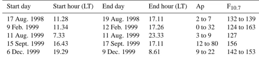
Table 1. Characteristics of the five experiments (decimal hours).
Start day Start hour (LT) End day End hour (LT) Ap F10.7
17 Aug. 1998 11.28 19 Aug. 1998 17.11 2 to 7 132 to 139 9 Feb. 1999 11.34 12 Feb. 1999 17.26 0 to 32 124 to 163 11 Aug. 1999 7.33 11 Aug. 1999 23.33 3 to 9 127 15 Sept. 1999 16.43 17 Sept. 1999 17.11 12 to 80 156 6 Dec. 1999 19.29 9 Dec. 1999 8.61 9 to 22 142 to 153
compute the corresponding modelled electron density pro-files and the modelled TEC was compared to incoherent scat-ter (IS) radar measurements. This study indicated that when
hmF2 and NmF2 data were available – but not the whole
electron density – ionosonde data might be successfully used with profilers to retrieve the electron density profile and the TEC (see also Huang and Reinisch, 2001 and Belehaki et al., 2003). The intercomparison of ionosondes and positioning systems (at the same location) would also provide an indi-rect measurement of the protonosphere, located between the upper altitude of the profiler modelling (about 3000 km) and the altitude of the GPS satellites (22 200 km).
In this paper we undertake a further comparison of ionosonde and EISCAT data at times when GPS-TEC mea-surements were also available. The study particularly ad-dresses the intercalibration of the IS radar electron density (see also Sedgemore et al., 1998).
2 Data sources
Ionosonde data have been obtained from two instruments lo-cated on the Tromsø EISCAT site, namely the Dynasonde and the Digisonde (DGS) (Reinisch et al., 1992). For the observations in this paper the Digisonde and the Dynasonde typically operated every 12 min with the parameters foF2 – being an estimate of the highest frequency with ordinary po-larisation reflected from the F2-region – and hmF2. Both have been automatically scaled on both instruments. The for-mer is related to NmF2 according to f oF2=8.98
√ N mF2, where foF2 is in Hz and NmF2 is in electrons m−3. The Digisonde data were autoscaled and were then manually scaled as a check. Weak echoes were obtained on many oc-casions making interpretation difficult.
In this paper, we focus on EISCAT data from the Tromsø UHF (931 MHz) radar (e.g. Rishbeth and Van Eyken, 1993). The details of the background theory have been reviewed in Bauer (1975). The analysis of the scattered signal provides height profiles of the ion and electron temperature, the ion velocity parallel to the magnetic field line, and the electron density. From the electron density profile, the true-height of the peak, corresponding to hmF2, its density value, sponding to NmF2, and therefore its plasma frequency, corre-sponding to foF2 can be determined. We call these quantities
foF2(IS) and NmF2(IS).
The calibration to absolute density must be done by com-parison with other techniques. Once done, this calibration is in principle valid for a long period, assuming no changes to the radar hardware.
3 EISCAT – GPS comparison: origin of the problem
In a recent study Lilensten and Cander (2003) found five pe-riods with common EISCAT and GPS observations at the Tromsø site and in this paper, we again focus on these peri-ods which correspond to well calibrated GPS-TEC and EIS-CAT CP1 data availability. In this EISEIS-CAT mode, the Tromsø beam is pointing parallel to the local magnetic field line. The integration time for processing the raw data is 1 or 2 min. The measurement of the ionospheric profiles is performed be-tween 90 and 498 km with a computational accuracy of ∼5% for the electron densities (Lathuill`ere, 1994; Lathuill`ere et al., 2002). These five experiments cover 257.75 h during 15 days. Table 1 shows that the experiments cover a wide range of solar and magnetic activities, from very quiet to dis-turbed.
The source of GPS data is the International GPS Service for Geodynamics receiver at Tromsø. TEC estimates along all GPS satellite links in view for elevation angles greater than 10◦are derived using a technique developed by Ciraolo (1993, 2000) and described recently in detail by Cander and Ciraolo (2002). Assuming a single-layer approximation for the ionosphere, these slants TEC data are then converted to equivalent vertical values at the intersection point of the ray-path with an ionospheric shell fixed at 400 km height. The conversion of the slant TEC to the vertical TEC may of course be a source of error, especially at high latitudes where the shell approximation can break down. The accuracy of the TEC deduced from GPS data is of the order of 2 TECU (1 TECU=1016electrons.m−2).
Figure 1 shows a comparison between GPS-TEC and the IS-TEC498 (IS-TEC498 denotes TEC up to a height of
498 km) derived from the EISCAT measurements. This last value has not been corrected by ionosonde calibration. In several cases, the TECs are close to or even smaller than the IS-TEC498– see, for example, 15 to 17 September 1999.
This should never happen, since the radar observes between the ground and 498 km while the GPS-TEC is an integra-tion between the ground and 20 200 km. In order to make
J. Lilensten et al.: Comparison of EISCAT and ionosonde electron densities 185
Fig. 1. Comparison between GPS TEC (thin lines) and the ISTEC498 derived from the uncalibrated EISCAT measurements
(bold lines).
sure that this is not an artefact of the uncalibrated IS data, it is necessary to compare the uncalibrated IS radar data with ionosonde data.
4 EISCAT–ionosonde comparisons
In this study, the Digisonde only has two common periods, 15–17 September 1999, and part of 6–9 December 1999. The Dynasonde data covers all five experimental periods.
In the following figures, we show comparisons between the IS measurements and the ionosondes. We compare foF2, the squared ratio being the correction factor that should be used for the IS-TEC. For ease of plotting, the hours are local time (LT) on the first day of the experiment, LT + 24 on the second day, LT + 48 on the third day, etc.
For the period 15–17 September 1999 (Fig. 2) foF2 is gen-erally closer to the IS measurements than the Dynasonde but both ionosondes give values smaller than those measured by the IS radar. When the least reliable ionosonde mea-surements have been eliminated, the mean foF2(NmF2) ra-tio between the ionosonde and the IS-foF2 is 1.1 (1.23) for the Dynasonde and 1.07 (1.14) for the Digisonde. When we
Accepted for publication in Annales Geophysicae - 2004
V12 - dated 28 July 2004
1
15 – 17 September 1999
Fig. 2. foF2 comparison between the IS radar data (black), the
Dy-nasonde (red) and the DGS (green). The top panel shows the ratio between the ionosonde-foF2 data and the IS-foF2 data in the same colour scheme.
combine the data from both ionosondes and keep the points temporally closest to the IS points, the ratio is 1.01.
For the period 6–9 December 1999 (Fig. 3) we obtain the opposite behaviour: both ionosondes estimate foF2 to be higher than the IS radar. The Digisonde data were only avail-able for the last two days of the experiment. On average, the
foF2 ratio between the Dynasonde and the IS-measurement
is 0.91 (0.83) and 0.88 (0.77) with the Digisonde. When we use the data from both ionosondes and keep the points tem-porally closest to the IS points, the ratios are 0.94 (0.88).
For the period 17–19 August 1998 (Fig. 4) we only have data from the Dynasonde (red). It gives a ratio of 1.13 (foF2) or 1.28 (NmF2). This ratio is computed with the part of the experiment shown in the upper panel of Fig. 4 but even when we include the complete period (and, therefore, some less reliable points), the ratio remains approximately the same.
The 9–12 September 1999 experiment (Fig. 5) is one of those where the TEC measured by the IS radar is very close to the TEC obtained from the GPS signals. It is interesting to notice that the foF2 measured by the Dynasonde fluctu-ates around the foF2 measured by the radar. On average, the ratio is very close to 1. However, if we were using a ratio
186 J. Lilensten et al.: Comparison of EISCAT and ionosonde electron densities
Accepted for publication in Annales Geophysicae - 2004
V12 - dated 28 July 2004
1
15 – 17 September 1999
6 – 9 December, 1999
Fig. 3. foF2 comparison between the IS radar data (black), the
Dy-nasonde (red) and the DGS (green).
dependent on time, we would obtain an increase of the IS-TEC498 when it is already close to or larger than the GPS
data. This is especially true during the period 65 LT to 75 LT (i.e. 11 February, around 20 LT).
The agreement between the ionosonde and the IS-foF2 is almost perfect during most of the 11 August 1999 experi-ment (Fig. 6) but at the end of the experiexperi-ment, the ionosonde critical frequency drops faster than that from the IS radar.
The drop corresponds to weak echoes and non-continuous traces such that the cusp near the penetration frequency is not properly measured. Under such conditions the ionograms may not give foF2 reliably, this being most likely due to ab-sorption, possibly compounded by broadcast or other inter-ference.
5 Effect of ionosonde calibration on the IS-TEC esti-mates
We conclude that if we calibrate EISCAT using the ionosonde measurements, we should use the following fac-tors: 17–18 August: 1.28; 9–12 February: 1; 11 August: 1; 15–17 September: 1.14; 6–9 December: 0.83.
Accepted for publication in Annales Geophysicae - 2004
V12 - dated 28 July 2004
2
17 – 19 August 1998
9 – 12 February 1999
Fig. 4. foF2 comparison between the IS radar data in black andthe IS-ionosonde in red. In the upper panel, the full line shows the points that have been kept to compute the mean ratio.
Figure 7 is similar to Fig. 1 but now we plot the IS-TEC498
measured by the EISCAT after correction by the ionosondes together with the TEC measured by GPS.
Even after calibration, the periods when the IS-TEC498is
larger than the GPS-TEC remain. Moreover, the last exper-iment in December 1999 (bottom panel) shows that the IS data are sometimes identical to the GPS data, which is im-possible, since the IS measures only up to 498 km while the satellites measure between the ground and 22 200 km. This last experiment is the only one to have a correction factor smaller than 1. The ratio between GPS-TEC and IS-TEC is about 2 before correction and 1.7 afterwards. A value of ∼2 would be expected because the electrons below 500 km, on the one hand, and in the range 500–22000 km, on the other hand, account for half of the total each (Lilensten and Blelly, 2002).
6 Interpretation
There may be practical reasons for observing discrepancies between the ionosondes and the IS radar measurements of
J. Lilensten et al.: Comparison of EISCAT and ionosonde electron densities 187
Accepted for publication in Annales Geophysicae - 2004
V12 - dated 28 July 2004
2
17 – 19 August 1998
9 – 12 February 1999
Fig. 5. foF2 comparison between the IS radar data in black and the
Dynasonde.
is wider than that associated with EISCAT measurements. Ionosonde echoes are only returned from regions where the refractive index surface lies perpendicular to the ray path. In a spherically stratified ionosphere this is a relatively nar-row region overhead, appropriate to the Fresnel radius at the measurement frequency. In a nonuniform ionosphere signals can originate from off the vertical - indeed from several re-gions – none of which necessarily correspond to the EISCAT volume. The ionosonde echo might originate from localised high-density structures which may result in an foF2 measured by ionosonde that is higher than a measurement based on the mean density measured by EISCAT.
By comparison, EISCAT measures the average density in a narrower cone: the EISCAT aperture is 0.9◦and the height integration in the F-region is 3 km with the power profile data and 22.5 km with the long pulse. In other words, EISCAT measures in a volume, whereas ionosondes measure reflec-tion heights which are relatively thin, but within large areas. In selecting the echoes from the Dynasonde to compare with the IS radar, there was no strict requirement that the echoes should come from exactly within the EISCAT vol-ume, but most echoes had a direction of arrival of less than 20◦from zenith.
11 August 1999
Fig. 6. foF2 comparison between the IS radar data in black and the
Dynasonde (red).
The discrepancies, although small, between the two ionosondes located only 100 m apart raises another issue. Ionospheric absorption, perhaps by underlying auroral-E, broadcast or other radio interference, can limit the strength and quality of echoes. The determination of foF2 depends on the strength of the echoes, on the software and hardware which registers these echoes and on the quality of the au-tomatic or human data reduction approach, especially under conditions of spread-F.
As shown in this study, the calibration of the EISCAT In-coherent Scatter radar through ionosonde data is not a trivial task. However, it is important to calibrate EISCAT as often as possible, even continuously. The best way to proceed is to use the plasma line (Perkins and Salpeter, 1965; Perkins et al., 1965). In principle, it is a measurement that can be made by any IS radar, provided that the plasma line is enhanced by photo- or auroral electrons or artificially by high-power HF waves. It is directly linked to the absolute electron den-sity, but varies in strength with time and altitude. Most of the plasma lines experiments have been difficult to perform be-cause the plasma line can vary quickly (Nilsson et al., 1996; Guio et al., 1998). The new data-taking program tau2 pl at EISCAT now allows for routine measurements of the plasma
188 J. Lilensten et al.: Comparison of EISCAT and ionosonde electron densities
Fig. 7. Comparison between the TECs derived from the GPS
sta-tions (thin lines) and the calibrated ISTEC498derived from the EIS-CAT measurements (bold lines). Only the three corrected periods are shown.
line and, therefore, the direct and continuous calibration of the ion line.
The importance of ionosonde and GPS measurements to the Space Weather programme is well accepted. However, a better understanding the generality of both TEC derived from
hmF2 and NmF2 profilers and GPS instrumentation used in
regions where the thin shell approximation is likely to break down is needed. The IS technique provides a third refer-ence technique to study this. Therefore, we suggest that it is important to (i) calibrate several IS radars with the plasma line technique, and (ii) compare GPS, ionosonde and IS radar data over a large set of cases in order to better understand the differences.
Acknowledgements. We are grateful to I. Galkin from the Lowell Digisonde team for Digisonde data analysis and to B. Pibaret for the EISCAT data processing. EISCAT is an International Associ-ation supported by the Research Councils of Finland (SA), France (CNRS), Japan (NIPR), Germany (MPG), Norway (NFR), Sweden (VR) and the United Kingdom (PPARC).
Topical Editor M. Lester thanks a referee for his/her help in evaluating this paper.
References
Bauer, P.: Theory of waves incoherently scattered, Phil. Trans. R. Soc. Lond, A, 280, 167–191, 1975.
Belehaki, A., Jakowski, N., and Reinisch, B. W.: Comparison of ionospheric ionization measurements over Athens using ground ionosonde and GPS derived TEC values, Rad. Sci., 6, 1105– 1112, 2003.
Cander, Lj. R. and Ciraolo, L.: First step towards specification of plasmaspheric-ionospheric conditions over Europe on-line, Acta Geod. Geoph. Hung., 37, 153–161, 2002.
Ciraolo, L.: Evaluation of GPS L2-L1 biases and related daily TEC profiles, Proceedings of the GPS/Ionosphere Workshop, Neustre-litz, 90–97, 1993.
Ciraolo, L.: Results and problems in GPS TEC evaluation, Proceed-ings of the Radio Communications Research Units, 1st GPS TEC Workshop, Chilton, 47–60, 2000.
Galkin, I. A., Kitrosser, D. F., Kecic, Z., and Reinisch, B. W.: In-ternet access to ionosondes, J. Atmos. Solar-Terr. Phys. 61, 181– 186, 1999.
Guio, P., Lilensten, J., Kofman, W., and Bjorna, N.: Electron veloc-ity distribution function in a plasma with temperature gradient and in the presence of suprathermal electrons: application to in-coherent scatter plasma lines, Ann. Geophys., 16, 1226–1240, 1998,
SRef-ID: 1432-0576/ag/1998-16-1226.
Hagfors, T.: Plasma fluctuations excited by charged particle motion and their detection by weak scattering of radio waves, Incoher-ent scatter, theory, practice and science, edited by Alcayd´e, D., Technical report 97/53, EISCAT scientific association, 1997. Huang, X. and Reinisch, B. W.: Vertical Electron Content from
Ionograms in Real Time, Radio Science, 36, 2, March/April, 335–342, 2001.
Killeen, T. L., Skinner, W. R., Johnson, R. M., et al.: The TIMED Doppler interferometer (TIDI), SPIE, 3756, 289–301, 1999. Lathuill`ere, C.: Intercomparisons between wind and temperature
measurements by WINDII (O1S) observations and EISCAT in-coherent scatter radar, Proceedings of the Workshop “Wind Ob-servations in the Middle Atmosphere”, CNES, Paris, France, 1994.
Lathuill`ere, C., Gault, W., Lamballais, B., Rochon, Y. J., and Sol-heim, B.: Doppler Temperatures from O1D airglow in the day-light thermosphere as observed by the WINDII interferometer on board the UARS satellite, Ann. Geophys., 20, 203–212, 2002,
SRef-ID: 1432-0576/ag/2002-20-203.
Leitinger, R.: Ionospheric electron content – the European perspec-tive, Ann. di Geofisica 41, 743–755, 1998.
Lilensten, J.: A review of some ionospheric and thermospheric processes relating to space weather, Space Weather Work-shop: Looking towards a European Space Weather Programme, ESTEC, Netherland, 2001.
Lilensten, J. and Blelly, P. L.: The TEC and F2 parameters as tracers of the ionosphere and thermosphere, J. Atm. Sol. Terr. Phys., 64, 775–793, 2002.
Lilensten, J. and Cander, Lj. R.: Calibration of the TEC derived from GPS measurements and from ionospheric models using the EISCAT radar, J. Atm. Sol. Terr. Phys., 65, 833–842, 2003. Nilsson, H., Kirkwood, S., Lilensten, J., and Galand, M.: Enhanced
incoherent scatter plasma lines, Ann. Geophys., 14, 1462–1472, 1996,
SRef-ID: 1432-0576/ag/1996-14-1462.
J. Lilensten et al.: Comparison of EISCAT and ionosonde electron densities 189
fluctuations by nonthermal electrons, Phys. Rev. A, 139, 55–62, 1965.
Perkins, F. W., Salpeter, E. E., and Yngvesson, K. O.: Incoherent Scatter from Plasma Oscillations in the Ionosphere, Phys. Rev. Lett., 14, 579–581, 1965.
Pick, M., Lathuillere, C., and Lilensten, J.: Ground Based measurements, WP 3120, ESA Space Weather study, http://www.estec.esa.nl/wmwww/wma/spweather/ esa initiatives/spweatherstudies/spweatherstudies.html, 2001. Reinisch, B. W., Haines, D. M., and Kuklinski, W. S.: The new
portable Digisonde for vertical and oblique sounding, NATO-AGARD, CP502, (11)1–11, 1992.
Rishbeth, H. and Van Eyken, A. P.: EISCAT : early history and the first ten years of operation, J. Atmos. Terr. Phys., 55, 525–542, 1993.
Sedgemore, K. J. F., Williams, P. J. S., Jones, G. O. L., and Wright, J. W.: Plasma drift estimates from the Dynasonde: comparison with EISCAT measurements, Ann. Geophys., 16, 1138–1143, 1998,