HAL Id: hal-00004549
https://hal.archives-ouvertes.fr/hal-00004549
Submitted on 22 Mar 2005
HAL is a multi-disciplinary open access
archive for the deposit and dissemination of
sci-entific research documents, whether they are
pub-lished or not. The documents may come from
teaching and research institutions in France or
abroad, or from public or private research centers.
L’archive ouverte pluridisciplinaire HAL, est
destinée au dépôt et à la diffusion de documents
scientifiques de niveau recherche, publiés ou non,
émanant des établissements d’enseignement et de
recherche français ou étrangers, des laboratoires
publics ou privés.
NGC1333-IRAS2
Valentine Wakelam, C. Ceccarelli, Alain Castets, Bertrand Lefloch, Laurent
Loinard, Alexandre Faure, N. Schneider, Jean-Jacques Benayoun
To cite this version:
Valentine Wakelam, C. Ceccarelli, Alain Castets, Bertrand Lefloch, Laurent Loinard, et al.. Sulphur
chemistry and molecular shocks: the case of NGC1333-IRAS2. Astronomy and Astrophysics - A&A,
EDP Sciences, 2005, 437, pp.149-158. �10.1051/0004-6361:20042566�. �hal-00004549�
ccsd-00004549, version 1 - 22 Mar 2005
(DOI: will be inserted by hand later)
Sulphur chemistry and molecular shocks: the
case of NGC1333-IRAS2
V. Wakelam
1, C. Ceccarelli
2, A. Castets
1, B. Lefloch
2, L. Loinard
3, A. Faure
2,
N. Schneider
1, J-J. Benayoun
21 L3AB Observatoire de Bordeaux, BP 89, 33270 Floirac, France
2 Laboratoire d’Astrophysique, Observatoire de Grenoble - BP 53, F-38041
Grenoble cedex 09, France
3 Centro de Radioastronom´ia y Astrof´isica, Universidad Nacional Aut´onoma de
M´exico, Apartado Postal Postal 72-3 (Xangari), 58089 Morelia, Michoac´an,
Mexico
Received 17 December 2004 / Accepted 23 February 2005
Abstract. We present SO and SO2 observations in the region of the low mass
protostar IRAS2/NGC1333. The East-West outflow originating from this source
has been mapped in four transitions of both SO and SO2. In addition, CS
obser-vations published in the literature have been used. We compute the SO, SO2and
CS column densities and the physical conditions at several positions of the outflow
using LTE and a non-LTE LVG approximations. The SO2/SO and CS/SO
abun-dance ratios are compared with the theoretical predictions of a chemical model adapted to the physical conditions in the IRAS2 outflow.
The SO2/SO abundance ratios are constant in the two lobes of the outflow
whereas CS/SO is up to 6 times lower in the shocked gas of the East lobe than in the West one. The comparison with the chemical model allows us to constrain
the age of the outflow produced by IRAS2 to ≤ 5 × 10³ yr. We find low densities
and temperatures for the outflow of IRAS2 (< 106 cm−3 and ≤ 70 K) from SO
and SO2 emission probably because the two molecules trace the cooled entrained
material. The East lobe of the outflow shows denser gas compared to the West lobe. We also discuss some constraints on the depleted form of sulphur.
Key words.ISM: abundances – ISM: molecules – Stars: formation – ISM: jets and
1. Introduction
Accretion and ejection are two apparently antithetic phenomena occurring simultane-ously during the first stages of star formation. Both are vital in the overall process: the former for the central object to grow, the latter to eliminate the excess angular momen-tum, and to allow accretion to proceed. In the very first phases of star formation, the ejection occurs through collimated, fast and extended flows of material, often probed by molecular rotational lines, and therefore refered to as molecular outflows and/or jets. Indeed, the forming star being still embedded in the parental molecular cloud, the out-flowing gas strikes the ambient material, often causing molecular shocks at the interaction interface. These shocks can be and indeed often are so violent that the grain mantles are partially destroyed, so that some heavy elements, usually frozen onto the grain surfaces, are released into the gas phase. Depending on the shock velocity, magnetic field and pre-shock density, the pre-shocks may dissociate the existing molecules (J-type pre-shocks: Hollenbach & McKee 1989), or, on the contrary, form many molecules in the “gently” shocked gas (C-type shocks: Draine 1980; Flower & Pineau des Forˆets 2003), or in the post-shocked gas. The SiO molecule represents a representative case in this respect (Schilke et al. 1997), but several other molecules have been observed to have abundances much greater in molecular shocks than in molecular clouds (e.g. Bachiller 1996). The time scale of the ejection process compared to the protostar life is not well known. To date the outflows there are two possible methods. One is dynamical and uses the ejected matter velocity (based on the line profiles) and the distance from the protostar. An other way to con-strain the age of shocks is to study their chemical evolution through chemical clocks. Chemical clocks are abundant species whose abundance depends more on time compared with the dynamical evolution of the source. Thus comparing the observed abundances of these species with their theoretical evolution should indicate the age of the shocked region.
Sulphur-bearing species are of particular interest, for the following two reasons: a) Sulphur is known to be severely depleted in molecular clouds, where its measured abundance is 1000 times less than the cosmic abundance (Tieftrunk et al. 1994). Note that the sulphur depletion likely occurs in the molecular cloud phase because in the diffuse medium the total abundance of sulphur in the gas phase is close to the cosmic abundance of S. On the other hand, SO, SO2 and H2S are often abundant in
molecu-lar shocks (Bachiller & Perez Gutierrez 1997; Codella & Bachiller 1999; Wakelam et al. 2004b); therefore S-bearing molecules can be potentially good shock tracers;
b) Sulphur chemistry is relatively fast, with typical timescales of some 104yr (Wakelam
et al. 2004a); therefore, the relative abundances of “appropriate” S-bearing molecules could in principle be used to date the outflows (Bachiller et al. 2001).
These two properties have long been recognized and several theoretical studies have fo-cused on the use of sulphur-bearing species as “chemical clocks” (Charnley 1997; Hatchell et al. 1998; Bachiller et al. 2001; van der Tak et al. 2003; Wakelam et al. 2004b,a). Several observational studies have targeted the “hot cores” of protostars, regions where the dust mantles evaporate because of the elevated dust temperature. Unfortunately, Wakelam et al. (2004a) have demonstrated that the use of S-bearing molecules as chemical clocks is far from easy. The main difficulty is that, indeed, the time evolution of the S-bearing species abundances critically depends on the initial form of the sulphur on the grain mantles, and on the exact physical conditions of the gas. As a result, it is very difficult to estimate the age of sources belonging to different molecular clouds since the initial sulphur composition could be very different and mask any evolutionary effect on the S-bearing species abundances. It is, however, still possible that the abundance of S-S-bearing molecules in shocked gas belonging to the same system (outflow source and molecular cloud) can be used to date the different shock sites. At least, one can expect that this would be easier to interpret than in the case of hot cores of different sources. In other words, a system where ejection events occurred at different times and caused successive shock sites could be a good benchmark for a time-dependent sulphur chemistry study. For this reason we decided to study an outflow system where multiple ejection events are suspected to have occurred. The basic question we want to answer is: can the (relative) abundance of sulphur-bearing molecules identify shocks that occurred at different times? The article is organized as follows. We describe the selected outflow system (§2), the ob-servations (§3), the obtained maps (§4) of the most abundant S-bearing molecules in the region and the derived relative abundances along the outflow (§5). In §6 we describe the chemical model (Wakelam et al. 2004a) applied to the outflow system studied. Finally, in §7, we discuss the results and compare the observed abundances with the predictions of the chemical model.
2. NGC1333-IRAS2: source background
The selected source, IRAS2, is situated in the NGC1333 molecular cloud, an active star forming region at 220 pc (Cernis 1990), with several low- and intermediate-mass protostars (Aspin et al. 1994; Lada et al. 1997). Evidence of the interaction between the protostars and the parental cloud (like H2 jets, Herbig-Haro objects and molecular
outflows) have been widely reported (Bachiller & Cernicharo 1990; Sandell et al. 1994; Blake et al. 1995; Warin et al. 1996; Langer et al. 1996; Ward-Thompson et al. 1996; Lefloch et al. 1998a,b; Bachiller et al. 1998; Knee & Sandell 2000). NGC1333 hosts a few very young Class 0 sources only detectable in the millimeter to FIR wavelength range (Jennings et al. 1987).
Among them, IRAS2 (IRAS 03258+3104 source of the IRAS Point Source Catalogue) is a low mass Class 0 protostar located at the edge of a cavity (Langer et al. 1996). IRAS2 is indeed composed of three continuum components: A, B and C. The B and C components (IRAS2B and IRAS2C) are respectivelly at 30′′ South-East and 30′′
North-West of the A component (IRAS2A) (Looney et al. 2000; Knee & Sandell 2000). In practice, IRAS2A is the most studied source among the three, and it is often refered to as IRAS2 (Sandell et al. 1994). In the following, we will follow this tradition of calling IRAS2 the A component.
Two bipolar outflows in the North-South and East-West directions emanate from IRAS2, suggesting that it is a non-resolved binary system (Sandell et al. 1994). The North-South outflow was first detected by Liseau et al. (1988) in the CO 1 - 0 transition. Later on, Sandell et al. (1994) showed that this outflow is not very collimated (see also Knee & Sandell 2000, for a detailled study of this outflow). These authors also discovered another outflow coming out from IRAS2 and oriented East-West. This outflow is very powerful, collimated and has a high inclination in the plane of the sky, which makes the East and West lobes spatially well separated (Bachiller et al. 1998). Using interferometric maps of the CH3OH emission, Bachiller et al. (1998) have proposed that the lobes of this outflow
are composed of several bullets, created in successive mass loss episodes. They predicted a difference of ∼ 2 × 10³ yr between the farthest and nearest bullets.
We obtained maps of the IRAS2 East-West outflow system in four transitions of SO and SO2 respectively. The first goal is to estimate the gas temperature and density as
well as the column density of SO and SO2 along the outflow. We also re-computed the
CS column densities along the outflow, using the line emission maps previously published in Langer et al. (1996). The ultimate goal is to compare the SO/SO2/CS ratios observed
along the outflow with the predictions of the chemical model by Wakelam et al. (2004a), and to estimate the age of the shocks along the outflow.
3. Observations
The IRAS2 region was observed with the IRAM 30m telescope at Pico Veleta (near Granada, Spain) during several runs in January and August 1998 and January 1999. We performed large-scale maps at a sampling of 12′′ in the following molecular transitions:
SO (32 → 21, 23 → 12, 43 → 32 and 65 → 54 transitions) and SO2 (31,3 → 20,2,
101,9→100,10, 51,5 →40,4 and 52,4→41,3 transitions). We covered an area of ∆α × ∆δ
= 228′′×96′′in SO and 216′′×84′′in SO
2. The relative coordinates (∆α, ∆δ) used in all
the maps presented here refer to the source IRAS2 (α(2000.0) = 3h28m55s41, δ(2000.0)
= 31014′35.08′′). Table 1 summarizes the relevant parameters of the observed transitions.
All observations were performed using the position switching mode, with an off posi-tion at ∆α = +70′′and ∆δ = +190′′from the nominal position of IRAS2 in NGC 1333.
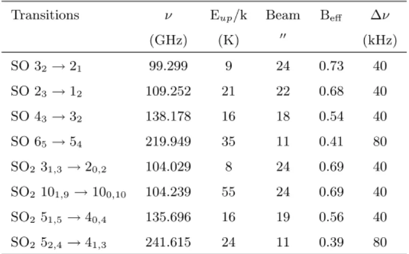
Table 1. Parameters of the observed SO and SO2 transitions: the frequency (ν), the
energy of the upper level divided by the Boltzmann constant (Eup/k), the telescope
beam, the beam efficiency of the telescope (Beff) and the spectral resolution (∆ν).
Transitions ν Eup/k Beam Beff ∆ν
(GHz) (K) ′′ (kHz) SO 32→21 99.299 9 24 0.73 40 SO 23→12 109.252 21 22 0.68 40 SO 43→32 138.178 16 18 0.54 40 SO 65→54 219.949 35 11 0.41 80 SO231,3→20,2 104.029 8 24 0.69 40 SO2101,9→100,10 104.239 55 24 0.69 40 SO251,5→40,4 135.696 16 19 0.56 40 SO252,4→41,3 241.615 24 11 0.39 80
This position is void of molecular emission since it corresponds to the center of the molec-ular cavity described in Langer et al. (1996). Pointing was checked every 1-2 hrs on the nearby continuum source 0333+321. The pointing accuracy was found to be better than 3′′. An autocorrelator split into three parts was connected to three receivers working at
1, 2 and 3 mm respectively, allowing simultaneous observations of three different transi-tions. The achieved spectral resolution is ≤ 0.12 km s−1. The weather conditions were
very good, and typical system temperatures were in the range of 120, 200 and 300 K at 3, 2 and 1.3 mm respectively. The spectra were calibrated with the standard chopper-wheel method and are reported here in units of main-beam brightness temperatures.
4. Results
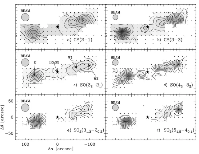
Figure 1 displays the integrated intensity maps of the SO 32→21and 43→32 lines, as
well as the SO231,3→20,2and 51,5 →40,4 lines, and, for comparison, the CS 2 → 1 and
3 → 2 lines (Langer et al. 1996). Three peaks of emission stand out on the maps: one associated with the East lobe of the outflow (marked E in the map - offset 72′′, -12′′) and
two associated with the West lobe (marked W1 -offsets -60′′, 12′′- and W2 -offset -96′′,
24′′- respectively). On the contrary, no enhanced emission is observed towards the source
itself with the exception of the CS 3 → 2 line. The E and W2 regions are symmetrically situated around IRAS2, and have previously been identified by Langer et al. (1996)1 as
the bow shocks at the end of the East and West lobes of the outflow. The three positions E, W1 and W2 coincide with peaks of CH3OH emission (Bachiller et al. 1998).
For a proper comparison of the spectra taken at different frequencies, all spectra were smoothed to the same spatial resolution of 24′′, which corresponds to the largest beam
1 The CS 5 → 4 line has also been observed but is seldon detected. Thus, we did not use it
Fig. 1.Integrated intensity maps of the CS 2 → 1 (a) CS 3 → 2 (b) SO 32→21 (c) SO
43 →32 (d) SO2 31,3 → 20,2 (e) and SO2 51,5 → 40,4 (f) transitions. (a), (b), (c) and
(d) : first level is 0.5 K km s−1 with level step of 2.5 K km s−1. (e) and (f): first level is
0.2 K km s−1 with level step of 0.3 K km s−1. The CS data are taken from Langer et al.
(1996) whereas the SO and SO2 data are from this work. In each map, the black points
represent the observed positions. The star shows the position of the protostellar source IRAS2. The arrows point to the positions whose spectra are displayed in Fig. 2.
(including the CS observations from Langer et al. 1996). Note that the SO2 51,5 →40,4
and 52,4 →41,3 spectra at the IRAS2 position were not smoothed because of the lack
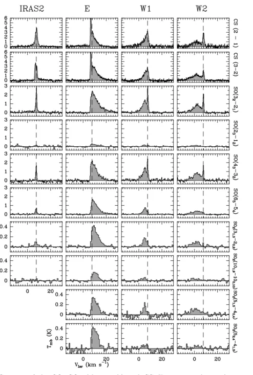
of observed positions around the source. However, since the target of the present study is the outflow and not the source itself, this is not relevant. The spectra of the SO and SO2 transitions observed towards IRAS2, E, W1 and W2 are shown in Fig. 2, and the
derived line parameters are summarized in Table 2.
As already noticed, the emission of the SO and SO2lines is strongly enhanced in the E,
W1 and W2 positions, whereas it is very weak toward the protostar itself. In the direction of IRAS2, the spectra exhibit profiles similar to the ones observed in the molecular cloud: very narrow lines with an intensity decreasing with the energy of the line suggesting that the emission is dominated by the cloud rather than the source. Conversely, the spectra of the outflow regions are very intense and exhibit high-velocity wings. In the western positions (W1 and W2 in Fig. 2), two velocity components can be clearly seen. The first
Fig. 2. Spectra of the SO, SO2 (this work) and CS (Langer et al. 1996) transitions
observed toward IRAS2 and along the outflow, in the three positions E (72′′, −12′′),
W1 (−60′′, 12′′) and W2 (−96′′, 24′′) (see text). All shown spectra are smoothed at the
largest beam 24′′. The SO251,5→40,4and 52,4 →41,3toward IRAS2 are not represented
because they cannot be smoothed (see text). The vertical dashed line on each spectrum marks the position of the cloud systemic velocity (vLSR = 7.6 km s−1).
component, with a broad profile, is blue-shifted by 6 km s−1with respect to the velocity
of the ambient cloud. We will refer to this component as the High Velocity Component, “HVC”. The second component peaks at the systemic velocity of the cloud, 7.6 km s−1.
We will refer to this component as the Low Velocity Component, “LVC”. While the HVC component clearly probes the outflowing gas, the situation is less clear for the LVC
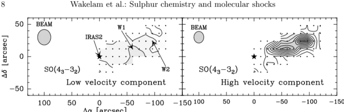
Fig. 3.Integrated intensity maps of the LVC and HVC SO 43→32transition separately
traced on the left and right panels respectively. The first level is 0.5 km s−1 with level
step of 1 km s−1.
component because the maps are not large enough. However, there is some indication that the LVC component is associated with the molecular cloud, for the LVC component is extended and is poorly contrasted (see Fig. 3). Also, the vLSR, 7.6 km s−1, is constant
across the emitting region. The lines of the East lobe (E) are brighter than those of the West lobe, and only one component is detected, red-shifted with respect to the systemic velocity. Most probably the component centered on the cloud velocity is buried of this red-shifted bright component, making it difficult to separate the two components. Similar profiles have been observed in the CS survey of NGC1333 by Langer et al. (1996).
Table 2 reports the velocity-integrated intensity in each position (the area under the Gaussian profile and integrated over the velocity interval at the “zero-intensity” level) which we will use to derive the gas temperature, density and species column densities. Note that we fitted separately the low (LVC) and high (HVC) velocity components. While this is easy for the West lobe emission where the two components are well separated, the fit is more tricky in the East lobe, where the two components are blended. In order to compute the area of the two components in the East lobe, we procede as follows. The LVC component is supposed to be centered on the systemic velocity of the cloud (7.6 km s−1) and to have a fixed width of 1 km s−1 (same width as the LVC component
of the West lobe). The residual spectrum, after removing the LCV component, is HVC. Using this method, the resulting LVC integrated intensity is less than 30% of the HVC one. Therefore, the uncertainty on HVC intensity produced by the mixing of the two components is low whereas the LVC one is less robust. For this reason, we will consider in the following only the HVC component of the East lobe.
Some but not all of the spectra of the West lobe can be fitted by two Gaussians, representing the LVC and HVC components respectively. On the contrary, none of the spectra of the East lobe can be analysed by two Gaussians. In those cases where the two Gaussian fit the line, it would be more correct to consider the line intensity of the LVC and HVC components computed in this way, rather than just integrating over two different velocity intervals, as explained above. However, since the two Gaussian
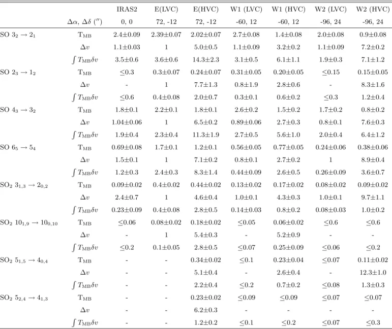
Table 2. Intensity (TMB) in K, velocity width (∆v) in km s−1 and integrated intensity
(RTMBδv) in K km s−1 of the SO and SO2 line profiles shown in Fig. 2. LVC and HVC
mean the low and the high velocity component of the spectra of the west lobe. The linewidth of E(LVC) is fixed to 1 km s−1 based on the linewidths of the West LVC
components because the LVC and HVC components of the East lobe are mixed.
IRAS2 E(LVC) E(HVC) W1 (LVC) W1 (HVC) W2 (LVC) W2 (HVC)
∆α, ∆δ (′′) 0, 0 72, -12 72, -12 -60, 12 -60, 12 -96, 24 -96, 24 SO 32→21 TMB 2.4±0.09 2.39±0.07 2.02±0.07 2.7±0.08 1.4±0.08 2.0±0.08 0.9±0.08 ∆v 1.1±0.03 1 5.0±0.5 1.1±0.09 3.2±0.2 1.1±0.09 7.2±0.2 R TMBδv 3.5±0.6 3.6±0.6 14.3±2.3 3.1±0.5 6.1±1.1 1.9±0.3 7.1±1.2 SO 23→12 TMB ≤0.3 0.3±0.07 0.24±0.07 0.31±0.05 0.20±0.05 ≤0.15 0.15±0.05 ∆v - 1 7.7±1.3 0.8±1.9 2.8±0.6 - 8.3±1.6 R TMBδv ≤0.6 0.4±0.08 2.0±0.7 0.3±0.1 0.6±0.2 ≤0.3 1.2±0.4 SO 43→32 TMB 1.8±0.1 2.2±0.1 1.8±0.1 2.6±0.2 1.5±0.2 1.7±0.2 0.8±0.2 ∆v 1.04±0.06 1 6.5±0.2 0.89±0.06 2.7±0.3 0.8±0.1 7.6±0.3 R TMBδv 1.9±0.4 2.3±0.4 11.3±1.9 2.7±0.5 5.6±1.0 2.0±0.4 6.4±1.2 SO 65→54 TMB 0.69±0.08 1.7±0.1 1.2±0.1 0.56±0.05 0.77±0.05 0.24±0.06 0.38±0.06 ∆v 1.5±0.1 1 7.1±0.2 0.8±0.1 2.7±0.2 1 8.9±0.4 R TMBδv 1.2±0.3 2.4±0.3 8.3±1.4 0.44±0.09 2.6±0.5 0.26±0.09 3.6±0.7 SO231,3→20,2 TMB 0.09±0.02 0.4±0.02 0.44±0.02 0.13±0.02 0.17±0.02 0.08±0.02 0.09±0.02 ∆v 2.4±0.7 1 4.6±0.4 1.0±0.1 4.3±0.3 1.0±0.1 9.7±1.1 R TMBδv 0.23±0.09 0.4±0.08 2.8±0.5 0.14±0.03 0.8±0.2 0.08±0.03 1.0±0.2 SO2101,9→100,10 TMB ≤0.06 0.08±0.02 0.18±0.02 ≤0.05 0.06±0.02 ≤0.6 ≤0.6 ∆v - 1 5.4±0.3 - 5.2±0.9 - -R TMBδv ≤0.2 0.1±0.05 2.8±0.5 ≤0.07 0.25±0.09 ≤0.06 ≤0.2 SO251,5→40,4 TMB - - 0.34±0.02 ≤0.1 0.23±0.04 ≤0.07 0.11±0.02 ∆v - - 5.1±0.4 - 2.6±0.4 - 12.3±1.0 R TMBδv - - 2.2±0.4 ≤0.2 0.7±0.2 ≤0.08 1.3±0.3 SO252,4→41,3 TMB - - 0.23±0.02 ≤0.09 ≤0.09 ≤0.07 ≤0.07 ∆v - - 6.2±0.3 - - - -R TMBδv - - 1.2±0.2 ≤0.1 ≤0.2 ≤0.07 ≤0.3
analysis is not possible everywhere, we decided to adopt the same method for all the points. While this choice does not practically affect the integrated intensity of the HVC component (the errors remain within the observational errors), it affects the LVC line intensity determination. To give the order of magnitude of the possible error associated with the adopted procedure, the two Gaussians analysis would give at most a factor of 2 lower integrated intensity for the SO lines, 20% less for the CS lines and no LVC component would be detected in the SO2lines. The consequencies for the computed LVC
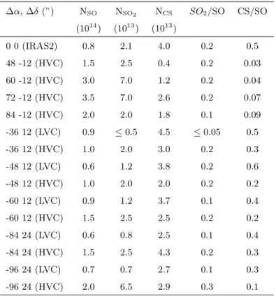
Table 3. Column densities of SO, SO2 and CS, as derived from an LVG analysis, at
several points along the outflow and on the source IRAS2 position The column densities (averaged on the 24′′beam) have been derived with a non-LTE LVG analysis (see text).
As we only have one SO2 transition detected on the source position, we used the same
temperature and density as for CS to derive the SO2column density on IRAS2. LVC and
HVC refer to the low and high velocity component respectively (see Sect. 4 for details). The uncertainties in the derived column densities are given by the observational errors, and are about 30%. Consequently, the uncertainty in the abundance ratios is about 60%. If we compute the LVC SO column densities with the LVG model using a temperature of 20 K and a density of 5 × 104cm−3 instead of the χ2method explained in section 5.2,
we find column densities two times higher than the ones reported in this table.
∆α, ∆δ (”) NSO NSO2 NCS SO2/SO CS/SO (1014) (1013) (1013) 0 0 (IRAS2) 0.8 2.1 4.0 0.2 0.5 48 -12 (HVC) 1.5 2.5 0.4 0.2 0.03 60 -12 (HVC) 3.0 7.0 1.2 0.2 0.04 72 -12 (HVC) 3.5 7.0 2.6 0.2 0.07 84 -12 (HVC) 2.0 2.0 1.8 0.1 0.09 -36 12 (LVC) 0.9 ≤0.5 4.5 ≤0.05 0.5 -36 12 (HVC) 1.0 2.0 3.0 0.2 0.3 -48 12 (LVC) 0.6 1.2 3.8 0.2 0.6 -48 12 (HVC) 1.0 2.0 2.0 0.2 0.2 -60 12 (LVC) 0.9 1.2 3.7 0.1 0.4 -60 12 (HVC) 1.5 2.5 2.5 0.2 0.2 -84 24 (LVC) 0.6 0.8 2.5 0.1 0.4 -84 24 (HVC) 1.5 2.5 4.3 0.2 0.3 -96 24 (LVC) 0.7 0.7 2.7 0.1 0.3 -96 24 (HVC) 2.0 6.5 2.9 0.3 0.1
section and reported in Tables A.1 and 3) are the following: NSO would be 30% to 40%
lower, NCSwould be 20% lower and the SO2/SO abundance ratios would have an upper
limit around 0.08 in the West LVC whereas the CS/SO abundance ratios would be almost the same as in Table 3. For this reason, our analysis will especially focus on the HVC emission, where the determination of the integrated emission is robust. On the contary, we will treat the LVC emission with more caution in the rest of the paper.
5. Column densities and abundance ratios
We estimated the column densities of the SO, SO2 and CS molecules and put some
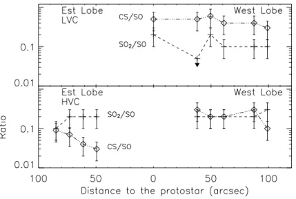
Fig. 4.SO2/SO and CS/SO abundance ratios (Table 3) as a function of the distance to
the protostar. Upper panel represents the LVC ratios of the West lobe (SO2/SO ratios
are upper limits). Lower panel shows the ratios in the HVC of East and West lobes. Note that the uncertainty in the values of the ratios is about 60%.
along the outflow. Both the rotational diagram method and a non-LTE LVG code were used. In this section, we present only a summary of the results. The details of this analysis are given in Appendix A.
For the LVC component, our modeling suggests densities between 2 × 10⁴ and 2 ×
105 cm−3 and temperatures about 25 K. Thus for the modeling of the chemistry (next
section), we will assume a density of 5 × 104 cm−3 and a temperature of 20 K for this
component. For the HVC component, we found a difference in the physical conditions between the two lobes of the outflow: the temperatures and densities derived from SO2
in the East lobe suggest a gradient along the outflow. We also found a slight difference between SO and SO2. Indeed, SO seems to probe a gas less dense that the gas probed
by the SO2 transitions, suggesting a spatial differentiation in the formation of these two
molecules. However, the data are not sufficient to better quantify this, so that in the following we will assume in our chemical modeling that both molecules originate in the same gas, where the density is around 105 cm−3and the temperature is about 50 K, the
median values between SO and SO2derivations.
The column densities derived using both methods differ by less than 30%. The column densities and the SO2/SO and CS/SO abundance ratios obtained with the LVG model
are summarized in Table 3 for the several positions in the outflow. The abundance ratios are shown as a function of the distance to the protostar in Fig. 4. Remarkably, the derived abundance ratios are different in the LVC and HVC components, which, therefore, differ
Table 4.Initial conditions for the chemical modelling. a Elemental abundances used to
compute the gas phase composition in molecular clouds (step 1). b Species contained in
grain mantles and sputtered in the gas phase in shocks (step 2). We took the abundances observed on grains in high mass protostars regions.c The cosmic abundance of sulphur
is 3 × 10⁵(Sofia et al. 1994). We used a 30 times lower abundance to take into account
the high depletion of sulphur in molecular clouds (Tieftrunk et al. 1994; Wakelam et al. 2004a).d We varied the amount of sulphur sputtered from the grain mantle (see text).
Ref: (1) Wilson & Rood (1994); (2) Cardelli et al. (1996); (3) Meyer et al. (1998); (4) Schutte et al. (1996); (5) Keane et al. (2001); (6) Chiar et al. (1996); (7) Boogert et al. (1998); (8) Palumbo et al. (1997); (9) upper limit from van Dishoeck & Blake (1998).
Elemental abundancesa
Species Abundance Ref.
He 0.28 (1)
O 6.5 × 10⁻⁴ (2)
C+ 2.8 × 10⁻⁴ (3)
S+c 1.0 × 10⁻⁶
Grain mantle compositionb
Species Abundance Ref.
H2O 10−4 (4) H2CO 4 × 10⁻⁶ (5) CH3OH 4 × 10⁻⁶ (6) CH4 10−6 (7) OCS 10−7 (8) H2S 10−7 (9) Sd 3 × 10⁻⁷−3 × 10⁻⁵
not only in the kinematics and gas temperature and density, but also in the chemical composition.
In the next section we will try to understand the differences in the chemical com-position of the LVC and HVC components, as well as the gradients observed along the outflow, comparing the observed ratios with the theoretical ratios of the Wakelam et al. (2004a) chemical model, predicted for the physical conditions described above.
6. Chemical model
In this section, we compare the abundance ratios found in the LVC and HVC components with the predictions the chemical model we developed recently to study the sulphur chem-istry (Wakelam et al. 2004a). Briefly, the model computes the evolution of the chemical composition of a gas at a fixed temperature and density, given an initial composition of the gas phase and of the grain mantles components released in the gas phase at time=0.
In this sense, it is a pseudo time-dependent model, for it does not take into account the physical evolution of the gas, but only the chemical evolution. For the specific case of the molecular shocks we model here, the shock is assumed to warm and compress the gas, giving rise to a sudden increase of the gas temperature and density. Also, the grain mantles are sputtered by the ions accelerated in the shock (e.g. Pineau de Forets et al. 1993) and/or destroyed by the collisions between grains (e.g. Jones et al. 1994). As a result, some or all the grain mantle components are injected into the gas phase at the shock passage. The model thus computes the gas chemical composition as a function of time, following those changes: gas density and temperature, as well as the gas chemical composition due to the grain mantle (partial) evaporation.
Note that the model does not aim to reproduce all the molecular abundances, but it specifically focuses on the sulphur chemistry. In this respect, it has the most up-to date and complete set of reactions involving S-bearing molecules.
In practice, in the present study the passage of the shock is simulated by a two-step process:
1) Before the shock, the gas composition is computed for a cloud with the density and temperature derived by the observations of the LVC, namely 5 × 104 cm−3 and 20 K.
The elemental abundances used for this step are summarized in Table 4. The age of the cloud is estimated by comparing the model predictions with the observed CS/SO and SO2/SO abundance ratios.
2) The cloud chemical composition computed in step 1 is used as the initial condition for step 2 computations. To the cloud composition, we add the grain mantle components released into the gas phase (see Table 4), and then the model follows the chemical evolution of the gas at 0.1−10×105cm−3and 25-120 K (namely a range of temperatures
and densities appropriate for the conditions found in the HVC). Following the results of Wakelam et al. (2004a), we assume that sulphur mainly evaporates in the H2S, OCS
and atomic form and we vary the amount of atomic sulphur released in the gas phase. Note that we also considered the possibility that sulphur evaporates in the molecular form S2 but as in the case of the hot cores (Wakelam et al. 2004a) the model with the
evaporation of S2 does not reproduce the observations in shocks. We will therefore not
discuss this case further.
In summary, we studied the influence of four parameters: the temperature, the density, the time since grain mantle sputtering and the amount of atomic sulphur released from the grains.
Observed CS/SO
Observed SO2/SO
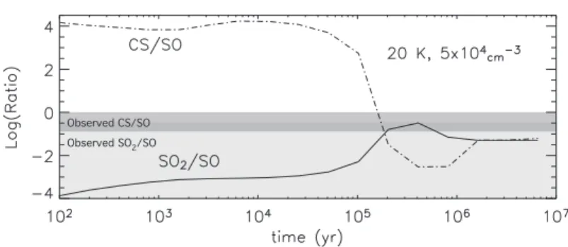
Fig. 5. Theoretical SO2/SO and CS/SO abundance ratios as a function of time. The
temperature is 20 K, and the density 5 × 104 cm−3. The two grey bands represent the
observed ratios in the LVC component of the East lobe (maximum and minimum values from Table 3 with the uncertainty of 50%). Note that for the SO2/SO ratio, we only have
a upper limit in the -36′′, 12′′LVC position. The darker band corresponds to the overlap
of the observed values.
6.1. Results: the cloud gas (LVC component)
Fig. 5 shows the SO2/SO and CS/SO abundance ratios as predicted by the chemical
model for the LVC temperature and density (20 K and 5 × 104 cm−3) as a function
of time. The observed ratios are reported on the same figure. The comparison between the model predictions and the observed ratios indicate that the cloud age is around 2 × 10⁵ yr or greater than about 106 yr. In that case, the observed SO
2/SO ratios are
in agreement with the model whereas the predicted CS/SO ratios are four times lower than the observed ones. An increase of the density or a decrease of the temperature leads to a better agreement between observed and predicted ratios. A decrease of the density or an increase of the temperature would have the opposite effect. For an age of 2 × 10⁵ yr, the model predicts absolute abundances 10 times higher than the observed
ones whereas the observed abundances are reproduced by the model within a factor of 3 for times longer than 106yr. This analysis assumes that SO, SO
2 and CS all originate in
the same gas, which in the case of the molecular cloud is likely a good approximation. As shown in Fig. 5, the CS/SO and SO2/SO ratios are each clocks that work differently
depending on the temperature and density. Indeed, because of the different dependence on the different model parameters, the use of both ratios can help constrain the age along with the density and temperature of the gas, as discussed above.
6.2. Results: the shocked gas
As we already mentioned, in addition to the temperature, the density and the time, we studied a fourth parameter: the amount of atomic sulphur injected in the gas phase which depends on the shock strengh. This last parameter, the amount of atomic sul-phur, is expected to be the same across the outflow. Consequently, we start studying the
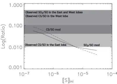
Fig. 6. Theoretical SO2/SO (solid line) and CS/SO (dash dot line) abundance ratios
as a function of the initial amount of atomic sulphur evaporated in the gas phase. We varied the amount of atomic sulphur (abundance compared to H2) evaporated in the
gas phase between 3 × 10⁻⁷ and 3 × 10⁻⁵. All the other model parameters are fixed:
T=50 K, n(H2)=105cm−3t=2000 yr. The two grey bands represent the observed ratios
in the shocked gas of the East and West lobes (see Table 3). Note that the two bands are superimposed in the middle (Log(Ratio)=0.004-0.1).
dependence of the predicted abundance ratios on this parameter. We took the average density and temperature previously derived by the SO emission in the HVC, namely 105 cm−3 and 50 K respectively. Anticipating the results on the time dependence of the
predicted ratios, we took an early time, 2000 yr. For these conditions, we ran several models, varying the initial amount of atomic sulphur. Fig. 6 shows the results of the modelling together with the range of observed ratios in the two lobes of the outflow. The first robust result is that only a small fraction of the sulphur is evaporated in the gas phase: ≤ 1/100 of the elemental sulphur in the West lobe and ≤ 1/40 of the elemental sulphur in the East lobe. This suggests that the shocks in IRAS2 are rather mild. The second result is that H2S and OCS evaporate from the grain more easily than atomic
sulphur. Indeed, decreasing the OCS injected in the gas by the same amount as S would give predictions not in agreement with the observations, because the abundance of CS in the warm shocked gas highly depends on the initial abundance of OCS. The decrease of H2S does not influence the results significantly. We will discuss this point further in
Sect. 7.
Taking the above composition for the injected material, we explored the dependence of the SO2/SO and CS/SO abundance ratios as function of the other three parameters
of the model: the density, temperature and age of the shock. The results are shown in Fig. 7.
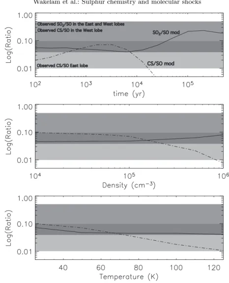
Fig. 7.Theoretical SO2/SO and CS/SO abundance ratios as a function of three
param-eters: time (upper panel), the H2 density (middle panel) and the temperature (lower
panel). In each panel, the other parameters are fixed: T=50 K and n(H2)=105cm−3 in
the upper panel, T=50 K and t=2000 yr in the middle panel, and n(H2)=105cm−3 and
t=2000 yr in the lower panel. For all the figures, the initial amount of evaporated atomic sulphur is 3 × 10⁻⁷. The two grey bands represent the observed ratios in the shocked gas
of the East and West lobes.(see Table 3). Note that the two bands are superimposed in the middle (Log(Ratio)=0.004-0.1).
The SO2/SO ratio depends weakly on the shock age, until 104yr, and on the density
and temperature of the shocked gas. On the contrary, the CS/SO ratio increases with time for (2 − 3) × 103yr before decreasing sharply because SO is efficiently produced whereas
the abundance of CS does not change. The CS/SO also decreases with the density, for nH2 ≥105 cm−3 and with the temperature. The CS/SO ratio is therefore an efficient
constraint on the shock age, temperature and density. We will discuss the constraints derived along the outflow in Sect. 7.
Finally, we notice that the HVC chemical modelling depends on the initial gas phase composition computed in step 1 (see Sect. 6), because the gas temperature (50 K) is
too low to reset the chemistry as is the case for the hot cores. In addition, the CS/SO ratio depends more on the initial composition than the SO2/SO ratio because CS is also
directly influenced by the initial abundance of atomic carbon (wich is a function of the cloud age). Indeed, the initial abundances are parameters hard to constrain, which we decided not to alter. The absolute abundances depend even more on the model parameters than the abundance ratios. Indeed, we are not able to reproduce the observed absolute abundances which are two orders of magnitude higher than the modelled ones. This discrepancy can have various causes. The first is that the modelling is wrong, and only further observations will be able to rule out this possibility. Other possibilities include the uncertainty on the adopted density and temperature. Here we are using average values across each modeled point, but there may be a stratification of density, temperature and chemical composition, that may affect the results. Also, the derived absolute abundances are rather uncertain because they are based on observations of low J CO transitions and this may be the most important cause of the discrepancy between the model and the observations. These observations have relatively large beams, and the amount of gas probed by the CO lines can be substantially larger than the gas where the SO, SO2and
CS lines are emitted, even up to a factor of 100. Only high spatial resolution observations will be able to clartify this possibility. In addition, the CO 2-1 line used to derive the H2
column density may be optically thick, underestimating the H2 column density, and only 13CO observations will be able to clarify this point. In the absence of such observations
we think that our modelling, based on the molecular abundance ratios -which are more robust than the absolute abundances- gives a reasonable and consistent interpretation of the observations. We will try to explore in detail the consequences of this interpretation in the next section.
7. Discussion
7.1. Nature of the LVC component
The density and temperature derived in the LVC (Sect. A.3) are consistent with the hypothesis suggested in §4, that the LVC is associated with the molecular cloud. Indeed, observations of the extended12CO and13CO emission suggest a density of ∼ 105 cm−3
and temperature of ∼ 20 K for the gas cloud (see Warin et al. 1996; Bergin et al. 2003). Likely, this gas is rather in the warm layers just behind the PhotoDissociation Region created by the illumination from a G0∼100 − 400 FUV field (see discussion in Bergin
et al. 2003). The SO column density in the LVC component is about 5 − 9 × 1013 cm−2,
which would translate into a SO abundance of about 0.6 − 1 × 10⁻⁹, assuming that the
warm layers extend for about 8 × 1022 cm−2 as derived by Warin et al. (1996). This
Hirahara et al. 1995) and the modeling of them (Wakelam et al. 2004a), so that we are tempted to conclude that the LVC component is dominated by the cloud emission.
Also from a chemical point of view, the SO2/SO and CS/SO ratios observed in LVC
seem to reflect the cloud chemistry, even though the chemical model predicts a CS/SO ratio lower than what is observed.
Finally, the constraints on the cloud age given by the sulphur chemistry, i.e. ∼ 2 × 10⁵yr or ≥ 106yr, are remarkably in agreement with previous estimates from Lada et al.
(1996), ≤ (1 − 2) × 106 yr, obtained by analysing Near-IR survey data. Therefore, the
cloud hosting IRAS2/NGC1333 is chemically young, less than 106yr old.
7.2. Age and physical conditions of the outflow
The comparison between the observed abundance ratios and the chemical modelling presented in Sect. 6 gives some constraints on the shock age, density and temperature. First, the sulphur bearing species indicate an age of 5 × 10²−7 × 10³ yr for the outflow
of IRAS2. This age is in agreement with the range estimated by Bachiller et al. (1998), 4 × 10²−5 × 10³ yr, based on the dynamics of the bullets of the IRAS2 outflow. The
estimated age of the outflow is also in agreement with the general scheme of formation and destruction of molecules in shocks proposed by Wakelam et al. (2004a, , Table 7): the simultaneous presence of SO and SO2would indicate a relatively young shock (≤ 103yr).
The accuracy on the SO2/SO and CS/SO ratios is however not good enough to constrain
the age of each clump and therefore to test if they are different events. The density of the HVC component in the West lobe is constrained by the CS/SO ratios to be lower than 2 × 105 cm−3 and the temperature lower than 70 K. These physical conditions are in
remarkable agreement with the non-LTE analysis of the SO emission presented in Sect. 5 (Table A.2). No constraints on the temperature or density can be deduced for the HVC component in the East lobe. However, the chemical modelling shows that an increase of the density and/or of the temperature leads to smaller CS/SO ratios. Thus, the lower CS/SO ratios observed in the East lobe compared with the West part of the outflow can be explained by a denser and/or warmer gas. The study of molecular excitation conditions (Table A.2) seems to confirm that the gas in the East lobe is denser than in the West lobe.
The density and temperature we derived in HVC are lower than that obtained by Jørgensen et al. (2004, 70 K and 106cm−3). For the temperature, we are still within the
mutual uncertainties. For the density value, we are forced to conclude that 106cm−3is not
in agreement with the HVC SO and SO2emission data since a high density would require
gas temperatures too low, similar to the rotational temperatures (in Table A.1). Indeed, we showed that optically thick lines cannot explain these low rotational temperatures (see Annex). One possible explanation for the different results by Jørgensen et al. (2004) is
that they did not consider the two lobes of the outflow separately, and also they treated all the studied molecules without studying the excitation conditions of each molecule individually. As we showed, the physical conditions are different in the East and West lobes, and different molecules probably trace different layers of shocked gas (see also Bachiller et al. 2001). In any case, the SO and CS densities computed by Jørgensen et al. (2004) are similar to ours in both LVC and HVC.
The low temperature (≤ 70 K) derived in the HVC component from SO and SO2
emission, and from other molecular emission by Jørgensen et al. (2004), as well as the small fraction of sulphur released in the shocked gas found from the chemical modelling suggest mild shocks. The SO, SO2and CS molecules seem rather to trace the entrained
material, mildly shocked, rather than the shock from the outflowing wind. This would explain both the lack of gas compression and the low gas temperature.
7.3. Consequences for the depleted form of sulphur
In this work on sulphur chemistry in shocks, we assumed that sulphur was sputtered from the grains in the OCS, H2S and S forms. This assumption does not imply that
sulphur is depleted in the atomic form but that the third form of depleted sulphur is quickly converted into S once evaporated in the gas phase. We denote this species S?.In Wakelam et al. (2004a), we proposed that S? is a polymeric form of sulphur such as S8.
One conclusion of this work is that it is more difficult to sputter S? than OCS and H2S. The efficiency of each molecule sputtering depends on the binding energy of that
molecule. Thus S? should have a higher binding energy than OCS and H2S. Unfortunatly,
this parameter is poorly known and depends highly on the grain surface composition.
8. Conclusions
We studied the SO, SO2 and CS emission in the protostar IRAS2 region and its
East-West outflow. Using both LTE and non-LTE methods, we computed the species column densities of the gas associated with the outflow and the ambient medium respectively. The computed CS/SO and SO2/SO abundance ratios were compared with the predictions
of a chemical model. The results are:
- The sulphur bearing emission is similar in the IRAS2 position and in the ambient medium whereas it is enhanced in the shocked regions at the interface between the cloud and the wind.
- The low velocity component (LVC) of the sulphur bearing spectra reflects the physical conditions and the chemistry of the cloud younger than 106 yr.
- The chemical modelling suggests that the IRAS2 outflow is young (≤ 2 × 10³ yr) but
time each clump of the outflow. The density of the gas traced by SO and SO2is lower
than 2 × 105 cm−3 and the temperature lower than 70 K in the West lobe. The gas
density in the East lobe is higher.
- The theoretical modeling suggests than SO and SO2 trace different layers of gas
and the entrained material rather than the shock itself. Thus, these molecules are not appropriate to study the physical conditions of the gas and the evolution of the outflow. CS on the contrary seems to be more sensitive to these parameters and the use of CS/SO ratios can help in understanding the molecular shocks associated with the outflows.
- Sulphur-bearing species depleted on the grain mantles may be more difficult to sputter than OCS and H2S. Thus, this species should have a higher binding energy than OCS
and H2S.
Acknowledgements. We thank the IRAM staff in Pico Veleta for their assistance with the
ob-servations, and the IRAM Program Committee for their award of observing time. V.Wakelam wishes to thanks Guillaume Pineau des Forˆets for helpful discussions.
References
Aspin, C., Sandell, G., & Russell, A. P. G. 1994, A&AS, 106, 165 Bachiller, R. 1996, ARA&A, 34, 111
Bachiller, R. & Cernicharo, J. 1990, A&A, 239, 276
Bachiller, R., Codella, C., Colomer, F., Liechti, S., & Walmsley, C. M. 1998, A&A, 335, 266
Bachiller, R., P´erez Guti´errez, M., Kumar, M. S. N., & Tafalla, M. 2001, A&A, 372, 899 Bachiller, R. & Perez Gutierrez, M. 1997, ApJ Lett., 487, L93
Bergin, E. A., Kaufman, M. J., Melnick, G. J., Snell, R. L., & Howe, J. E. 2003, ApJ, 582, 830
Blake, G. A., Sandell, G., van Dishoeck, E. F., et al. 1995, ApJ, 441, 689
Boogert, A. C. A., Helmich, F. P., van Dishoeck, E. F., et al. 1998, A&A, 336, 352 Cardelli, J. A., Meyer, D. M., Jura, M., & Savage, B. D. 1996, ApJ, 467, 334 Ceccarelli, C., Baluteau, J.-P., Walmsley, M., et al. 2002, A&A, 383, 603 Cernis, K. 1990, Ap&SS, 166, 315
Charnley, S. B. 1997, ApJ, 481, 396
Chiar, J. E., Adamson, A. J., & Whittet, D. C. B. 1996, ApJ, 472, 665 Codella, C. & Bachiller, R. 1999, A&A, 350, 659
Draine, B. T. 1980, ApJ, 241, 1021
Flower, D. R. & Pineau des Forˆets, G. 2003, MNRAS, 343, 390 Goldsmith, P. F. & Langer, W. D. 1999, ApJ, 517, 209
Green, S. 1995, ApJS, 100, 213
Hatchell, J., Thompson, M. A., Millar, T. J., & MacDonald, G. H. 1998, A&A, 338, 713 Hirahara, Y., Masuda, A., Kawaguchi, K., et al. 1995, PASJ, 47, 845
Hollenbach, D. & McKee, C. F. 1989, ApJ, 342, 306
Jennings, R. E., Cameron, D. H. M., Cudlip, W., & Hirst, C. J. 1987, MNRAS, 226, 461 Jones, A. P., Tielens, A. G. G. M., Hollenbach, D. J., & McKee, C. F. 1994, ApJ, 433,
797
Jørgensen, J. K., Hogerheijde, M. R., Blake, G. A., et al. 2004, A&A, 415, 1021
Keane, J. V., Tielens, A. G. G. M., Boogert, A. C. A., Schutte, W. A., & Whittet, D. C. B. 2001, A&A, 376, 254
Knee, L. B. G. & Sandell, G. 2000, A&A, 361, 671 Lada, C. J., Alves, J., & Lada, E. A. 1996, AJ, 111, 1964 Lada, E. A., Evans, N. J., & Falgarone, E. 1997, ApJ, 488, 286 Langer, W. D., Castets, A., & Lefloch, B. 1996, ApJ Lett., 471, L111
Lefloch, B., Castets, A., Cernicharo, J., Langer, W. D., & Zylka, R. 1998a, A&A, 334, 269
Lefloch, B., Castets, A., Cernicharo, J., & Loinard, L. 1998b, ApJ, 504, L109+ Liseau, R., Sandell, G., & Knee, L. B. G. 1988, A&A, 192, 153
Looney, L. W., Mundy, L. G., & Welch, W. J. 2000, ApJ, 529, 477 Meyer, D. M., Jura, M., & Cardelli, J. A. 1998, ApJ, 493, 222
Palumbo, M. E., Geballe, T. R., & Tielens, A. G. G. M. 1997, ApJ, 479, 839
Pickett, H. M., Poynter, R. L., Cohen, E. A., et al. 1998, J. Quant. Spectrosc. Radiat. Transfer, 60, 883
Sandell, G., Knee, L. B. G., Aspin, C., Robson, I. E., & Russell, A. P. G. 1994, A&A, 285, L1
Schilke, P., Walmsley, C. M., Pineau Des Forets, G., & Flower, D. R. 1997, A&A, 321, 293
Schutte, W. A., Tielens, A. G. G. M., Whittet, D. C. B., et al. 1996, A&A, 315, L333 Sofia, U. J., Cardelli, J. A., & Savage, B. D. 1994, ApJ, 430, 650
Swade, D. A. 1989, ApJ, 345, 828
Tieftrunk, A., Pineau Des Forets, G., Schilke, P., & Walmsley, C. M. 1994, A&A, 289, 579
Turner, B. E., Chan, K., Green, S., & Lubowich, D. A. 1992, ApJ, 399, 114
van der Tak, F. F. S., Boonman, A. M. S., Braakman, R., & van Dishoeck, E. F. 2003, A&A, 412, 133
van Dishoeck, E. F. & Blake, G. A. 1998, ARA&A, 36, 317
Wakelam, V., Caselli, P., Ceccarelli, C., Herbst, E., & Castets, A. 2004a, A&A, 422, 159 Wakelam, V., Castets, A., Ceccarelli, C., et al. 2004b, A&A, 413, 609
Table A.1. Rotational temperatures and column densities of SO and SO2 computed
from the rotational diagrams of Fig. A.1. Note that the detected lines of SO2transitions
towards IRAS2, W1(LVC) and W2(LVC) are not numerous enough to construct the SO2
rotational diagram in these regions. Thus the SO2 column densities towards IRAS2 and
the LVC components (W1 and W2 LVC) are derived assuming LTE and an excitation temperature of 10 K. SO SO2 CO ∆α, ∆δ (′′) T rot(K) NSO(1014cm−2) Trot(K) NSO2(1013cm−2) NCO(1017cm−2) 0, 0 (IRAS2) 11 ± 3 0.9 ± 0.01 10 0.5 ± 0.2 72, -12 (E HVC) 13 ± 3 4.0 ± 0.4 28 ± 11 10 ± 1 0.75 -60, 12 (W1 LVC) 7.3 ± 0.2 0.8 ± 0.04 10 0.3 ± 0.07 -60, 12 (W1 HVC) 11.7±2.8 1.6±0.2 28.1±12.9 2.8±0.2 0.45 -96, 24 (W2 LVC) 7.2 ± 0.6 0.6 ± 0.07 10 0.2 ± 0.07 -96, 24 (W2 HVC) 12.5±1.6 2.6±0.1 19.6±7.1 3.2±0.3 MNRAS, 281, L53
Warin, S., Castets, A., Langer, W. D., Wilson, R. W., & Pagani, L. 1996, A&A, 306, 935 Wilson, T. L. & Rood, R. 1994, ARA&A, 32, 191
Appendix A: Determination of the column and physical densities
In this section we report the details on the estimates of the column densities of the SO, SO2and CS molecules at selected positions along the ouflow. We used both the rotational
diagram method and a non-LTE LVG code. The two methods and the relevant results are discussed separately in the following. We anticipate that they give values for the column densities that differ by less than 30%.
A.1. Rotational diagram method
As widely discussed in the literature (e.g. Goldsmith & Langer 1999), the rotational di-agram method rests on the assumption that the molecular levels are in local thermal equilibrium (LTE) and that the lines are optically thin. Using the four observed transi-tions of SO and SO2, we constructed rotational diagrams at the three positions E, W1
and W2, and at the IRAS2 position (see Fig. A.1). Note that we did not perform this analysis for the CS data because we have only two transitions available. The obtained SO and SO2 rotational temperatures and column densities are reported in Table A.1.
As previously found for CH3OH (Sandell et al. 1994; Bachiller et al. 1998), the
ro-tational temperatures are relatively low when compared to the expected temperatures in the shocked gas. Sandell et al. concluded that IRAS2 was the first example of a cold shock, while Bachiller et al. proposed that the CH3OH lines are subthermally excited.
Fig. A.1.Rotational diagrams of the SO and SO2 molecules in the direction of IRAS2,
E, W1 and W2 regions. In W1 and W2 we have constructed separate diagrams for the LVC and HVC components: W1(LVC), W1(HVC), W2(LVC) and W2(HVC) whereas in E, we give only the HVC component (see text). Stars and triangles correspond to the SO and SO2 observed data respectively.
Indeed, the gas temperature in the IRAS2 outflow is certainly higher (i.e. ≥ 60 K) than the rotational temperatures in Table A.1 since bright NH3(3,3) emission has been
detected towards the two lobes (see Bachiller et al. 1998). We therefore endorse the interpretation by Bachiller et al., and we demonstrate that this is also the case for the SO and SO2 molecules in Appendix B: the low rotational temperatures are simply due
to non-LTE effects.
A.2. Non-LTE LVG method
In order to take into account the expected non-LTE effects, we analysed the data by means of a non-LTE LVG (Large Velocity Gradient) code. The general details of the code are described in Ceccarelli et al. (2002). We included the molecular data and the collisional coefficients for the SO, SO2 and CS molecules, by taking the former from the
JPL Catalogue (http://spec.jpl.nasa.gov/; Pickett et al. 1998) and the latter from Green (1994), Green (1995) and Turner et al. (1992) respectively. Briefly, the used non-LTE LVG
Fig. A.2.χ2contour at 2σ (95.4% in confidence) of the LVC and HVC SO line emission
in the 5 positions of the West lobe (upper panels) and the HVC SO and SO2line emission
in the 4 positions in the East lobe (lower panels) compared to the non-LTE LVG code.
code computes the rotational line fluxes solving simultaneously the statistical equilibrium of the levels and the radiative transfer of the emitted photons. The approximation of the LVG consists of assuming that the photons emitted at any point of the medium either are absorbed in the immediate vicinity or they escape (this is the so-called photon escape formalism), because the different regions are moving at high velocities. In practice, the photons cannot be absorbed if their frequency -shifted by the Doppler effect- is outside the thermal width centered on the rest frequency of the transition. The LVG approximation assumes homogeneous and isothermal semi-infinite slab. Although this approximation is strictly correct in the presence of large velocity gradient, and the absence of temperature and density gradients, it is very often used to give a first estimate of the average gas density and temperature of the observed medium. In this work, we will use the non-LTE code in this way. More sophisticated models would be required for a more sophisticated analysis. However, given the quality of the obtained data, a greater sophistication of the analysis would be unjustified.
Table A.2. Temperatures and densities constrained by the SO and SO2 observed line
emission using a non-LTE LVG method (see text) for the different positions along the outflow. The last two columns summarise the temperatures and densities used to compute the CS column densities reported in Table 3.
SO SO2 Adopted for CS ∆α, ∆δ (′′) T (K) n (cm−3) T (K) n (cm−3) T (K) n (cm−3) 0 0 (IRAS2) - ≥2 × 10⁴ - - 20 5 × 10⁴ 48 -12 (HVC) - ≥2.5 × 10⁴ ≤35 ≥6.3 × 10⁶ 50 105 60 -12 (HVC) ≥30 3.1 × 10⁴ - 4.0 × 10⁵ 20-80 2.5 × 10⁵ - 6.3 × 10⁶ 50 105 72 -12 (HVC) - ≥5 × 10⁴ 20-50 5 × 10⁵ - 7.9 × 10⁶ 50 105 84 -12 (HVC) - ≥2.5 × 10⁵ ≤30 ≥1.2 × 10⁶ 50 105 -36 12 (LVC) 14 - 75 2.2 × 10⁴ - 2.5 × 10⁵ - - 20 5 × 10⁴ -36 12 (HVC) - ≥2.5 × 10⁴ - - 50 105 -48 12 (LVC) 14 - 130 2.2 × 10⁴ - 5.0 × 10⁵ - - 20 5 × 10⁴ -48 12 (HVC) ≥70 4 × 10⁴ - 1.6 × 10⁵ - - 50 105 -60 12 (LVC) 15 - 24 1.0 × 10⁵ - 2.2 × 10⁵ - - 20 5 × 10⁴ ≥25 2.8 × 10⁴ - 6.3 × 10⁴ -60 12 (HVC) ≥45 2.5 × 10⁴ - 1.2 × 10⁵ - - 50 105 -84 24 (LVC) ≤130 ≥2.2 × 10⁴ - - 20 5 × 10⁴ -84 24 (HVC) ≥60 2.8 × 10⁴ - 1.0 × 10⁵ - - 50 105 -96 24 (LVC) ≤55 ≥2.5 × 10⁴ - - 20 5 × 10⁴ -96 24 (HVC) - ≥2.5 × 10⁴ - - 50 105
The code has three free parameters to be constrained by comparing the model pre-dictions with observed data: the gas density and temperature and the column density of the species. Implicitly, we are assuming that the emission fills the beam (24′′) and the
observed linewidth, namely 4 and 5 km s−1 for HVC of SO and SO2 and 1 km s−1 for
LVC of both molecules. We ran several cases varying the SO and SO2 column densities
from 1013 to 1017 cm−2, the density between 104 and 107 cm−3 and the temperature
between 10 and 200 K. We then searched for the minimum χ2 in this 3-D space, where
the χ2 is defined as usual :
χ2= 1 N − 2 N X 1 (Observations − M odel)2 σ2
We computed the SO and SO2 column densities, as well as the temperature and
density of the gas in five and four positions of the west and east lobes of the outflow respectively (Tables 3 and A.2). These positions include the E, W1 and W2 regions discussed in previous sections.
Taking the species column densities with the lowest absolute χ2 (Table 3), we
con-strained the gas density and temperature by plotting the χ2 contour at 2σ (95.4% in
temperature and density can reproduce the observed fluxes, so that they are only ap-proximatively constrained. Table A.2 reports the kind of constraints we obtained at each studied position.
Having available only two transitions for CS we could not carry out a similar method to constrain the gas density and temperature and the CS column density simultaneously. We assumed instead the average density and temperature as suggested by the SO ob-servations and reported in Table A.2 (see the detailed discussion in section 5.3), and computed the CS column density consequently using the LVG model. The results are reported in Table 3. Note that CS having the same density and temperature as SO im-plies that the two species are also chemically related. This is a major assumption, which is partially supported by the theoretical predictions that, in dense and warm gas, CS is mainly formed by C + SO (thus SO and CS are chemically linked; Charnley 1997; Wakelam et al. 2004a). However, even our observations cast some doubt on the robust-ness of this assumption, for the SO and CS emissions in the maps are slightly displaced. Not having other possibilities, we will adopt this assumption, but in the following we will keep in mind the limits of the assumption used.
A.3. Modeling results
Gas temperature and density
The non-LTE analysis gives an indication of the gas density and temperature along the outflow and in the LVC and HVC components (Fig. A.2 and Table A.2), within the limits discussed in the previous section and summarized again at the end of this section. In the following, we discuss the two velocity components separately.
i) LVC component
Although it is difficult to constraint exactly (with the presented observations) the gas den-sity and temperature in this component, the plot in Fig. A.2 suggests densities between 2 × 10⁴and 2 × 105cm−3 and temperatures somewhat higher than 15 K. Complementary
CO J=2-1 line observations of the IRAS2 outflow indicate brightness temperatures of 20-22 K, which implies a gas kinetic temperature of about 25 K (Wakelam 2005 in prep). This is consistent with Warin et al. (1996) who derived a similar temperature (about 20 K) and a similar density (about 105 cm−3) for the ambient gas by using 13CO and
C18O observations with a larger beamsize (2.5 arcmin). Thus, for the modelling of the
chemistry (next section), we will assume a density of 5 × 104cm−3 and a temperature of
20 K for this component. ii) HVC component
Here, the temperatures and densities are higher than in the LVC component and different in the two lobes of the outflow. Indeed, the gas temperature and density in the two
lobes (East and West), and as derived from SO and SO2respectively, present a slightly
different behaviour. The temperature and density derived from SO2 in the East lobe
suggest a gradient along the outflow. The two positions of maximum SO2 emission at
(60′′, −12′′) and (72′′, −12′′) display the highest kinetic temperatures, whereas the other
points, at the edge of the emission peak, display higher densities and lower temperatures. The gas probed by the SO2 emission seems therefore warmed at the peak position, and
compressed around it. A similar behavior may also be present in the gas probed by the SO transitions but it is less evident. Remarkably, Fig. A.2 shows that the T-n curves of the SO transitions do not overlap the curves of the SO2 transitions. The SO data
seem to probe a gas less dense than the gas probed by the SO2 transitions, suggesting
a spatial differentiation in the formation of these two molecules. Indeed, the map of the emission extent of the HVC component suggests that the SO emission is more extended than the SO2. However, the data are not sufficient to better quantify this, so that in the
following we will assume in our chemical modeling that both molecules originate in the same gas, where the density is around 1 × 105 cm−3 and the temperature is about 50 K,
the median values between the SO and SO2derivations. The same applies for CS, which
is also assumed to originate in the same gas the SO and SO2. As previously mentioned
(§5.2), this is likely a rough approximation, but the available data do not allow a better refinement of the treatment.
iii) Column densities and abundance ratios
As anticipated, the column densities computed with the non-LTE LVG method (Table 3) are very similar to the ones derived by the rotational diagrams. They differ by less than 30% with the exception of the SO2 column density in W2(HVC) where the difference
reaches 50%. The uncertainty on this latter value is higher because two transitions of SO2were not detected in W2. Note that the SO and SO2transitions are predicted to be
optically thin at the derived column densities.
Using the derived column densities, we estimated the abundance ratios reported in Table 3 and shown as function of the distance from the protostar in Fig. 4. The absolute abundances were derived from the CO column density, assuming a standard CO to H2
abundance [CO] = 10−4, following Warin et al. (1996). We adopted the value estimated
by Warin et al. (1996) for the LVC : 8×1022cm−2. For the HVC, we took the CO column
densities obtained from complementary observations of the CO J=2-1 line for our study of the SiO emission in the IRAS2 protostellar outflow (Wakelam 2005, in prep). The CO column density was estimated assuming the levels to be populated according to LTE and the transition to be optically thin. This assumption is motivated by the fact that the CO profiles are similar to the CS 2-1 ones with a line width of 10-20 km s−1. However,
only13CO 2-1 observations could confirm this hypothesis and the real H
2column density
for the CO gas. The values in the HVC are close to 1017cm−2; they are summarized in
Table 4 and are in agreement with the values obtained by Bergin et al. (2003), averaged over a region of 4 arcmin size.
We derive the following average absolute abundances for SO, SO2 and CS
respec-tively : 9 × 10⁻¹⁰, 10−10and 4 × 10⁻¹⁰ in the LVC. We obtain much higher values in the
HVC : 2 × 10⁻⁷, 4 × 10⁻⁸ and 4 × 10⁻⁸ in the West lobe, and 3 × 10⁻⁷, 7 × 10⁻⁸ and
2 × 10⁻⁸in the East lobe. Unfortunatly, we cannot perform an accurate analysis at each
point because of the lack of observations. Therefore, we will use the abundance ratios for the subsequent modelling.
Remarkably, the derived abundance ratios are different in the LVC and HVC components, which, therefore, differ not only in the kinematics and gas temperature and density, but also in the chemical composition. The CS/SO ratio is 0.3-0.6 in the LVC component, with the ratio steadily decreasing going outward (across the outflow). On the contrary, the CS/SO ratio in the HVC component is much more variable: it is between 0.03 and 0.1 in the East lobe, and 0.1-0.3 in the West lobe, i.e. up to 6 times larger in the West lobe. Contrary to the LVC component, it increases going outward in both lobes, with the exception of the farthest point in the West lobe. However, the largest difference between the LVC and HVC components is seen in the SO2/SO ratio;
less than 0.005 in the LVC component and about 0.2 in the HVC component, almost constant along the outflow.
iv) Uncertainties
One has to keep in mind the various approximations/assumptions used when trying to interpret these results. First, in our analysis we assumed that the three molecules originate in the same gas, which may not be the case. Second, in practice we assumed that the emission fills the beam, or that the filling factor is the same for the three molecules. If the lines are optically thin this would give values (gas density and temperature, as well as the species column density) that are correct, but if the lines are optically thick this may not be the case. In practice, we estimate that the computed abundance ratios are likely uncertain by about 60%. Higher spatial resolution observations are required for better estimates.
Appendix B: Excitation conditions
In this appendix, we present a study of the SO and SO2 excitation in the shocked gas
using a LVG model and following the Bachiller et al. (1998) idea. In practice, we would like to understand what physical conditions can explain an underestimation of the rotational temperatures derived from the SO and SO2emission (section A.1). In addition, we studied
Fig. B.1.SO (left panel) and SO2 (right panel) rotational temperature as a function of
density computed for several kinetic temperatures between 60 and 100 K. We assumed the SO and SO2 column densities found in W1(HVC) (NSO = 1.5 × 1014cm−2 and
NSO2 = 3 × 1013cm−2) using rotational diagrams. See text for details.
log (N SO r e a l / NSO c o mpu te d ) log (N SO 2 r e a l / NSO 2 c om pu te d )
Fig. B.2. Left pannels: SO and SO2 rotational temperatures as a function of column
densities computed for several H2densities between 104and 107cm−3and a kinetic
tem-perature of 100 K. Right pannels: Error on the SO and SO2column densities computed
with rotational diagrams as a function of H2densities and for several column densities.
the robustness of the column densities derived with the rotational diagrams if the basic hypothesis of the method is not verified.
Using the SO and SO2 fluxes computed by the LVG model, we reconstruct
theo-retical rotational diagrams for different column densities, kinetic temperatures and H2
densities. From these rotational diagrams, we derived theoretical rotational temperatures and column densities. To compare the theoretical diagrams with the observed ones, we constructed them only using the LVG fluxes of the four observed transitions of SO and SO2. The rotational diagram method is based on the assumptions of local thermal