HAL Id: hal-02993705
https://hal.archives-ouvertes.fr/hal-02993705
Submitted on 10 Nov 2020
HAL is a multi-disciplinary open access
archive for the deposit and dissemination of
sci-entific research documents, whether they are
pub-lished or not. The documents may come from
teaching and research institutions in France or
abroad, or from public or private research centers.
L’archive ouverte pluridisciplinaire HAL, est
destinée au dépôt et à la diffusion de documents
scientifiques de niveau recherche, publiés ou non,
émanant des établissements d’enseignement et de
recherche français ou étrangers, des laboratoires
publics ou privés.
Sulphur and carbon isotopes towards Galactic centre
clouds
P. Humire, V. Thiel, C. Henkel, A. Belloche, J.-C. Loison, T. Pillai, D.
Riquelme, V. Wakelam, N. Langer, A. Hernández-Gómez, et al.
To cite this version:
P. Humire, V. Thiel, C. Henkel, A. Belloche, J.-C. Loison, et al.. Sulphur and carbon isotopes towards
Galactic centre clouds. Astronomy and Astrophysics - A&A, EDP Sciences, 2020, 642, pp.A222.
�10.1051/0004-6361/202038216�. �hal-02993705�
Astronomy & Astrophysics manuscript no. main ESO 2020c September 21, 2020
Sulphur and carbon isotopes towards Galactic centre clouds
P. K. Humire,
1V. Thiel,
1C. Henkel,
1, 2, 3A. Belloche,
1J.-C. Loison,
4T. Pillai,
1, 5D. Riquelme,
1V.
Wakelam,
6N. Langer,
1, 7A. Hernández-Gómez,
1R. Mauersberger,
1and K. M. Menten
11
Max-Planck-Institut für Radioastronomie, Auf dem Hügel 69, 53121 Bonn, Germany e-mail: [email protected]
2
Dept. of Astron., King Abdulaziz University, P.O. Box 80203, Jeddah 21589, Saudi Arabia 3
Xinjiang Astronomical Observatory, Chinese Academy of Sciences, 830011 Urumqi, China 4
Institut des Sciences Moléculaires (ISM), CNRS, Univ. Bordeaux, 351 cours de la Libération, F-33400, Talence, France
5
Institute for Astrophysical Research, 725 Commonwealth Ave, Boston University Boston, MA 02215, USA 6
Laboratoire d’astrophysique de Bordeaux, CNRS, Univ. Bordeaux, B18N, allée Geoffroy Saint-Hilaire, F-33615 Pes-sac, France
7 Argelander-Institut für Astronomie, Universität Bonn, Auf dem Hügel 71, 53121 Bonn, Germany Received xxx, yyy; accepted xxx, yyy
ABSTRACT
Context. Measuring isotopic ratios is a sensitive technique used to obtain information on stellar nucleosynthesis and chemical evolution.
Aims. We present measurements of the carbon and sulphur abundances in the interstellar medium of the central region of our Galaxy. The selected targets are the +50km s−1Cloud and several line-of-sight clouds towards Sgr B2(N). Methods. Towards the +50 km s−1Cloud, we observed the J =2–1 rotational transitions of 12C32S, 12C34S, 13C32S, 12
C33S, and13C34S, and the J =3–2 transitions of12C32S and 12C34S with the IRAM-30 m telescope, as well as the J =6–5 transitions of12C34S and13C32S with the APEX 12 m telescope, all in emission. The J =2–1 rotational transitions of12C32S,12C34S,13C32S, and13C34S were observed with ALMA in the envelope of Sgr B2(N), with those of 12C32S and12C34S also observed in the line-of-sight clouds towards Sgr B2(N), all in absorption.
Results. In the +50 km s−1Cloud we derive a 12C/13C isotopic ratio of 22.1+3.3
−2.4, that leads, with the measured 13C32S/12C34S line intensity ratio, to a 32S/34S ratio of 16.3+3.0
−2.4. We also derive the 32S/34S isotopic ratio more directly from the two isotopologues13C32S and13C34S, which leads to an independent32S/34S estimation of 16.3+2.1−1.7 and 17.9±5.0 for the +50 km s−1Cloud and Sgr B2(N), respectively. We also obtain a 34S/33S ratio of 4.3±0.2 in the +50 km s−1Cloud.
Conclusions. Previous studies observed a decreasing trend in the32
S/34S isotopic ratios when approaching the Galactic centre. Our result indicates a termination of this tendency at least at a galactocentric distance of 130+60−30pc. This is at variance with findings based on12C/13C,14N/15N and18O/17O isotope ratios, where the above-mentioned trend is observed to continue right to the central molecular zone. This can indicate a drop in the production of massive stars at the Galactic centre, in the same line as recent metallicity gradient ([Fe/H]) studies, and opens the work towards a comparison with Galactic and stellar evolution models.
Key words. Galaxy: abundances – Galaxy: centre – Galaxy: evolution – ISM: abundances – ISM: molecules – radio lines: ISM
1. Introduction
Studying stellar nucleosynthesis and chemical enrichment of rare isotopes of a given element at optical wavelengths is difficult because the observed atomic isotope lines are usually affected by blending (e.g. Hawkins & Jura 1987;
Levshakov et al. 2006;Ritchey et al. 2011). However, at ra-dio and (sub)millimeter wavelengths, transitions from rare isotopic substitutions of a given molecular species, called isotopologues, are well separated in frequency from their main species, typically by a few percent of their rest fre-quency.
While the relative abundances of C, N, and O isotopes provide information on carbon–nitrogen–oxygen (CNO) and helium burning, sulphur isotopes allow us to probe late evolutionary stages of massive stars and supernovae (SNe)
of Type Ib/c and II (oxygen-burning, neon-burning, and s-process nucleosynthesis) (Wilson & Rood 1994;Chin et al. 1996; Mauersberger et al. 1996), filling a basic gap in our understanding of stellar nucleosynthesis and the chemical evolution of the universe (e.g.Wang et al. 2013).
In the interstellar medium (ISM), atomic sulphur is thought to freeze out on dust grain mantles and to be later released from the grains due to shocks, leading to the for-mation of several molecular species in the gas phase, such as OCS, SO2, H2S, and H2CS (Millar & Herbst 1990), which
serve as both shock and high-mass star formation tracers in starburst galaxies (Bayet et al. 2008).
Among the sulphur-bearing compounds, CS (carbon monosulfide) is the most accessible molecular species: its lines are ubiquitous in the dense ISM and tend to be strong
at sites of massive star formation in the spiral arms of our Galaxy, in the Galactic centre (GC) region and in external galaxies (e.g.Linke & Goldsmith 1980;Mauersberger et al. 1989;Bayet et al. 2009;Kelly et al. 2015).
Sulphur has four stable isotopes:32S,33S,34S, and36S. Their solar system fractions are 95.018:0.750:4.215:0.017 (Lodders 2003), respectively. In the ISM, Chin et al.
(1996) found a relation between 32S/34S isotope
ratios and their galactocentric distance (DGC) of 32S/34S=(3.3±0.5)(D
GC/kpc)+(4.1±3.1) by using a
linear least-squares fit to the unweighted data, with a correlation coefficient of 0.84, while no correlation was obtained between 34S/33S ratios and D
GC. However, most
of the sources observed in that study are located within the galactocentric distance range 5.5 ≤ DGC ≤ 7.0 kpc, with
the minimum distance at 2.9 kpc from the Galactic centre. Therefore, it is important to also cover the inner region of the Milky Way to find out whether the trend proposed by Chin et al. (1996) is also valid for the inner Galaxy as has been reported for the 12C/13C (see e.g. Yan et al. 2019), 14N/15N (Adande & Ziurys 2012) and 18O/17O (Wouterloot et al. 2008;Zhang et al. 2015) isotopic ratios. The GC region harbours one of the most intense and luminous sites of massive star formation in the Galaxy, Sgr B2 (Molinari et al. 2014;Ginsburg et al. 2018). It pro-vides an extreme environment in terms of pressure, turbu-lent Mach number, and gas temperature (Ginsburg et al. 2016) over a much more extended region than encountered in star-forming regions throughout the Galactic disc ( Mor-ris & Serabyn 1996; Ginsburg et al. 2016; Schwörer et al. 2019;Dale et al. 2019). These conditions are comparable to those in starburst galaxies (Belloche et al. 2013; Schwörer et al. 2019). We therefore expect unique results in this GC study from sulphur ratios, which are a tool for tracing stel-lar processing (see Sect.6). For a compilation of sulphur ratios determined in our Milky Way, we refer to Tables 2 and 7 inMauersberger et al.(2004) andMüller et al.(2006), respectively.
As is true for our Galaxy, detections of 34S in
extra-galactic objects remain scarce. Some observations, also ac-counting for12C/13C ratios (using the double-isotope ratio
method, Sect.4.1.1) led to values of ∼16–25 and 13.5±2.5 for the 32S/34S ratio in the nuclear starbursts of NGC 253
and NGC 4945, respectively (Wang et al. 2004;Henkel et al. 2014), although the value for NGC 4945 might be underesti-mated due to saturation of the CS lines (Martín et al. 2010). A ratio of 20±5 was obtained for N159 in the Large Mag-ellanic Cloud (Johansson et al. 1994). At redshift z=0.89, a 32S/34S ratio of 10±1 has been derived using absorption lines from the spiral arm of a galaxy located along the line of sight (l.o.s.) towards a radio loud quasar (Müller et al. 2006).
In the present study we focus on the J =2–1 transitions of 12C32S (hereafter CS), 12C34S (hereafter C34S), 13C32S (hereafter13CS),12C33S (hereafter C33S), and13C34S, the
J =3–2 transitions of CS and C34S, and the J =6–5
transi-tions of C34S and 13CS, all observed together towards the
Sgr A Complex (see, e.g., Sandqvist et al. 2015). We have also studied absorption features caused by the envelope of Sgr B2(N) in the J =2–1 rotational transition of CS, C34S, 13CS and 13C34S, as well as CS and C34S absorption
fea-tures caused by l.o.s. clouds towards Sgr B2(N). These ab-sorption and emission profiles allow us to obtain 12C/13C and the missing 32S/34S ratios close to the Galactic
nu-cleus. Expanding the database for sulphur isotope ratios in the GC region is important in order to constrain models of stellar interiors as well as models of the chemical evolution of the Galaxy (e.g.Kobayashi et al. 2011).
The paper is organised as follows. In Sect.2we describe the observations. In Sect.3we describe in detail our targets. In Sect.4 we present measured opacities and isotopologue ratios from CS species, the modelling of our Sgr B2(N) data, and a comprehensive study of CS fractionation. In Sect.5
we compare our results with previous studies. In Sect.6we discuss the results in the context of trends with galactocen-tric distance and give some explanations for our findings, before summarising and concluding in Sect.7.
2. Observations
2.1. +50 km s−1Cloud
The +50 km s−1Cloud observations were conducted with the IRAM 30 m and the APEX 12 m telescopes over a pe-riod of 1.5 years, from 2015 May to 2016 September, un-der varying weather conditions. The observed position was EQ J2000: 17h45m50.20s, −28◦590
41.100 for both telescopes, and the representative spectral resolution was 0.6 km s−1. With the IRAM 30 m telescope, three frequency set-ups were observed with the E090 and E150 receivers in com-bination with the Fast Fourier Transform Spectrometer (FFTS, at 195 kHz resolution mode1). For the observations
presented in this paper, we covered the 93.2–100.98 GHz frequency range (CS, C34S, and C33S J =2–1) in one
set-up with the E090 receiver. In a separate E090 set-set-up, our tuning covered the frequency range 85.5-93.3 GHz (13CS
and13C34S J =2–1), while simultaneously the E150 receiver covered the frequency range from 143.5 to 151.3 GHz (for CS and C34S J =3–2). The observations were conducted in total power position switching mode. No spectral con-tamination was found in our off-source reference position (17h46m10.4s, −29◦070
0800). The main beam efficiencies for our IRAM 30 m measurements were computed using the Ruze formalism (Ruze 1966). Adopted values were 0.8 and 0.7 at 98 and 147 GHz, respectively2. We discarded data
taken under poor weather conditions (precipitable water vapour content (pwv) > 7 mm) by discarding data taken with system temperatures > 500 K. The representative half-power beam widths (HPBW) values are about 2500at 98 GHz and 1700at 147 GHz for the IRAM 30 m observa-tions.
The Atacama Pathfinder Experiment 12 m telescope (APEX) 12 m (Güsten et al. 2006) was used for observa-tions of the J =6–5 lines of the CS, 13CS, and 13C34S iso-topologues at roughly 280 GHz. The measurements were conducted simultaneously using the FLASH345 (Klein et al. 2014) receiver connected to the extended FFTS (XFFTS) backend. These observations were also executed in total power position switching mode and the same off-source ref-erence position, which was found to be clean. The HPBW was about 2200 at the observed frequency and the adopted main beam efficiency was 0.7.
All line intensities are reported in main beam brightness temperature units (TMB). While the spectral resolution was
1
http://www.iram.es/IRAMES/mainWiki/Backends 2
calculated following the table in https://www.iram.fr/ GENERAL/calls/w08/w08/node20.html
instrument dependent (between 0.4 and 0.6 km s−1 for the IRAM and 0.08 km s−1 for the APEX data), all spectra were smoothed to a resolution of 3 km s−1 for analysis.
The data were reduced with the GILDAS package3and required minimal flagging, followed by a baseline subtrac-tion of order two.
2.2. Line-of-sight clouds towards Sgr B2(N)
For Sgr B2(N), we used the Exploring Molecular Complex-ity with ALMA (EMoCA) survey (Belloche et al. 2016) that was performed with the Atacama Large Millime-ter/submillimeter Array (ALMA) in the direction of this source. The centre of the observed field (see Fig.1) lies in the middle (EQ J2000: 17h47m19.87s, −28◦2201600) be-tween the two main hot cores, N1 and N2, which are sep-arated by 400. 9 along the north–south direction, or around 0.19 pc in projection assuming a distance to the Galactic centre, Sgr A∗, of 8.122 kpc (Gravity Collaboration et al. 2018). The survey covers the frequency range from 84.1 to 114.4 GHz, which includes carbon monosulfide J =2–1 lines, with a spectral resolution of 488 kHz (1.7 to 1.3 km s−1) at a median angular resolution of 100. 6, or ∼0.06 pc. The
av-erage noise level is ∼3 mJy beam−1 per channel. Details of the calibration and deconvolution of the data are reported in Belloche et al. (2016, Sect. 2.2). For this work, we cor-rected the data for primary beam attenuation. Several iso-topologues of CS are detected in the EMoCA survey. To determine the32S/34S and 12C/13C isotopic ratios, we use four isotopologues: CS, C34S, 13CS, and 13C34S.
A list of the observed transitions of CS isotopologues and some associated parameters is given in Table1.
3. Sources
The +50 km s−1Cloud (also known as M–0.02–0.07, al-though the +50 km s−1Cloud could include additional molecular knots on its positive-longitude side; (Ferrière 2012)), observed here with IRAM and APEX, is a giant molecular cloud (GMC) of hook or indented-sphere shape, considered to be one of the most prominent high-mass star formation sites in the GC. It has a mass of ∼5×10⁵M ;
a density of 104–105cm−3; a gas temperature of 80–100 K
(from NH3, CH3CN, and CH3CCH; Güsten et al. 1985),
∼190 K (from H2CO,Ao et al. 2013), or 410±10 K (from
NH3,Mills & Morris 2013); and a dust temperature of 20–
30 K (Sandqvist et al. 2008). The energetics of at least a part of the +50 km s−1Cloud are influenced by the super-nova (SN) remnant Sgr A East (Ferrière 2012;Uehara et al. 2019). In CS emission, its dense core peaks at a l.o.s. dis-tance of 3±3 pc relative to the Galactic centre (Ferrière 2012), coincident with 1.2 mm observations (Vollmer et al. 2003, and references therein), and peaks at (∆α, ∆δ) ≈ (3.0,0
10.5) with respect to Sgr A∗, corresponding to ≈7±3 pc to
the east along the Galactic plane and 4.5±3 pc to the south from the Galactic plane (see the explanation for galactocen-tric Cartesian coordinates inFerrière 2012, and their Table 1).
With ALMA we have observed Sgr B2(N)orth, one of the sites of massive star formation associated with Sgr B2, the most massive cloud in our Galaxy. The whole Sgr B2 complex has a total mass of 107M
(Goldsmith et al. 1990)
3
https://www.iram.fr/IRAMFR/GILDAS
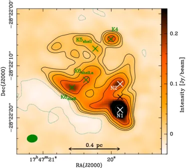
Fig. 1: ALMA continuum map of Sgr B2(N) at 85 GHz. The black contour lines show the flux density levels at 3σ, 6σ, 12σ, and 24σ and the dotted lines indicate -3σ, where σ is the rms noise level of 5.4 mJy beam−1. The white crosses denote the positions of the two main hot cores, Sgr B2(N1) and Sgr B2(N2). The black cross, located between the white ones, indicates the phase centre. The green crosses show peaks of continuum emission selected for our absorption study. They label the ultra compact H ii region K4, two peaks in the shell of the H ii region K6 and one peak in the shell of the H ii region K5 (Gaume et al. 1995). The green ellipse in the lower left corner shows the size of the synthesised beam of ∼100. 6 (see Table1).
and gas temperatures of at least 50 K (from p–H2CO in Ginsburg et al. 2016, their Sect. 5.8). Most of the mass in Sgr B2(N) (∼73%) is contained in one single core (AN01) (Sánchez-Monge et al. 2017). The densities and column den-sities of the hot cores in Sgr B2(N) are high (>106cm−3 and >1023cm2;Sánchez-Monge et al. 2017;Bonfand et al. 2019).
Sgr B2(N) is located at a galactocentric distance of 130+60−30pc from Sgr A∗ (from Reid et al. 2009, consider-ing the projected distance of 100 pc as lower limit) or ∼8 kpc from us. Its diameter is ∼0.8 pc (Lis & Goldsmith 1990;Schmiedeke et al. 2016). Several diffuse and translu-cent clouds are detected in absorption along the l.o.s. to Sgr B2(N) (see e.g. Greaves & Williams 1994; Thiel et al. 2019). The exact locations of the different velocity compo-nents of the l.o.s. clouds towards Sgr B2(N) are not yet fully constrained. In the case of our observations (see Table4), we can only suggest that the lines with negative velocities arise from l.o.s. clouds between the Expanding Molecular Ring (with a galactocentric radius of 200–300 pc, Whiteoak & Gardner 1979) and the 1 kpc disc, while the lines with posi-tive velocities arise from the envelope of Sgr B2(N) (Greaves & Williams 1994;Wirström et al. 2010;Thiel et al. 2019). Specifically, our lines in the range −105 to −70 km s−1 are believed to be located within 1 kpc of the GC (Corby et al.
Table 1: Some observational and physical parametersafor the five measured CS isotopologue transitions in the +50km s−1 Cloud and the four transitions from the l.o.s. clouds towards Sgr B2(N), which are also located in the Galactic centre region.
Target Telescope Isotopologue Transition ν0b Eup/kc Au,ld HPBWe
[GHz] [K] [s−1] [00] +50 Cloud IRAM 30 m 13C34S 2–1 90.9260260 6.55 1.19 × 10⁻⁵ 27.0 +50 Cloud IRAM 30 m 13CS 2–1 92.4943080 6.66 1.41 × 10⁻⁵ 26.6 +50 Cloud IRAM 30 m C34S 2–1 96.4129495 6.25 1.60 × 10⁻⁵ 25.5 +50 Cloud IRAM 30 m C33S 2–1 97.1720639 7.00 1.63 × 10⁻⁵ 25.3 +50 Cloud IRAM 30 m CS 2–1 97.9809533 7.05 1.67 × 10⁻⁵ 25.1 +50 Cloud IRAM 30 m C34S 3–2 144.6171007 11.80 5.74 × 10⁻⁵ 17.0 +50 Cloud IRAM 30 m CS 3–2 146.9690287 14.10 6.05 × 10⁻⁵ 16.6 +50 Cloud APEX 12 m 13CS 6–5 277.4554050 46.60 4.40 × 10⁻⁴ 22.1 +50 Cloud APEX 12 m C34S 6–5 289.2090684 38.19 4.81 × 10⁻⁴ 21.2 Sgr B2(N) ALMA 13C34S 2–1 90.9260260 6.55 1.19 × 10⁻⁵ 1.8×1.6 Sgr B2(N) ALMA 13CS 2–1 92.4943080 6.66 1.41 × 10⁻⁵ 2.9×1.5 Sgr B2(N) ALMA C34S 2–1 96.4129549 6.25 1.60 × 10⁻⁵ 1.9×1.4 Sgr B2(N) ALMA CS 2–1 97.9809533 7.05 1.67 × 10⁻⁵ 1.8×1.3
Notes. (a) The spectroscopic information for each molecule is taken from the Cologne Database for Molecular Spectroscopy (CDMS,Müller et al. 2005;Endres et al. 2016).(b)Rest frequency.(c)Upper energy level.(d)Einstein coefficient for spontaneous emission from upper u to lower l level. (e) Half-power beam width. For the IRAM sources it was calculated following Eq. 1 in
http://www.iram.es/IRAMES/telescope/telescopeSummary/telescope_summary.html.
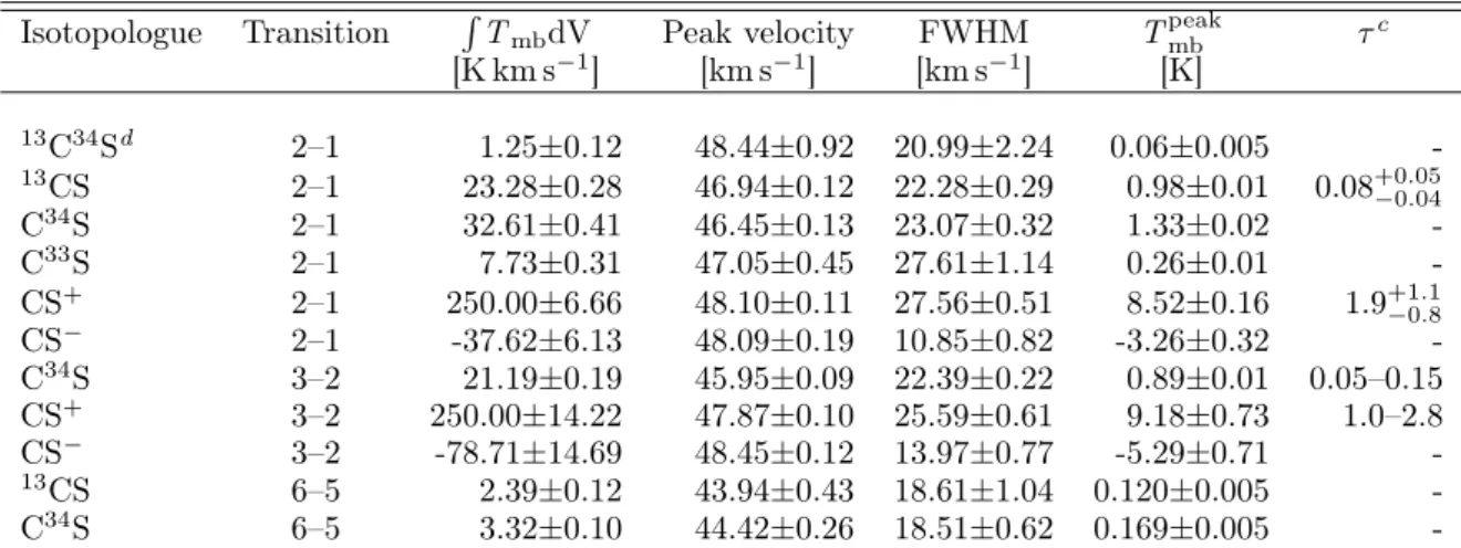
Table 2: Line parameters for the nine measured CS isotopologue transitions in the +50 km s−1Cloud. Isotopologue Transition R TmbdV Peak velocity FWHM T
peak mb τ c [K km s−1] [km s−1] [km s−1] [K] 13C34Sd 2–1 1.25±0.12 48.44±0.92 20.99±2.24 0.06±0.005 -13CS 2–1 23.28±0.28 46.94±0.12 22.28±0.29 0.98±0.01 0.08+0.05 −0.04 C34S 2–1 32.61±0.41 46.45±0.13 23.07±0.32 1.33±0.02 -C33S 2–1 7.73±0.31 47.05±0.45 27.61±1.14 0.26±0.01 -CS+ 2–1 250.00±6.66 48.10±0.11 27.56±0.51 8.52±0.16 1.9+1.1−0.8 CS− 2–1 -37.62±6.13 48.09±0.19 10.85±0.82 -3.26±0.32 -C34S 3–2 21.19±0.19 45.95±0.09 22.39±0.22 0.89±0.01 0.05–0.15 CS+ 3–2 250.00±14.22 47.87±0.10 25.59±0.61 9.18±0.73 1.0–2.8 CS− 3–2 -78.71±14.69 48.45±0.12 13.97±0.77 -5.29±0.71 -13CS 6–5 2.39±0.12 43.94±0.43 18.61±1.04 0.120±0.005 -C34S 6–5 3.32±0.10 44.42±0.26 18.51±0.62 0.169±0.005
-Notes.(c)Peak opacity .(d)a CH3OCH3(see Sect.4.1and Fig.2) contribution was subtracted before performing a single Gaussian fit to this line .(+)Positive component (in blue in Fig.2) .(−)Negative component (in green in Fig.2).
2018, and references therein), and our lines with veloci-ties around +60 km s−1are associated with the envelope of Sgr B2(N) (Wirström et al. 2010).
This massive star-forming region harbours five hot cores, namely Sgr B2(N1–N5), with kinetic temperatures ranging from ∼130 to 150 K for N3–N5, between 150 and 200 K for N2, and between 160 and 200 K for N1, assum-ing LTE conditions in all these cases (Belloche et al. 2016;
Bonfand et al. 2017;Belloche et al. 2019). In addition, there are 20 ∼1.3 mm continuum sources associated with dense clouds in Sgr B2(N) that exhibit a rich chemistry ( Sánchez-Monge et al. 2017; Schwörer et al. 2019). Recently, Gins-burg et al.(2018) detected 271 compact continuum sources at ∼3 mm in the extended Sgr B2 cloud, thought to be high-mass protostellar cores, representing the largest
clus-ter of high-mass young stellar objects reported to date in the Galaxy.
4. Results
In the following we first discuss the measured profiles to-wards the +50 km s−1 Cloud, and provide the equations used to determine peak opacities and the carbon isotope ratio (Sect.4.1). Then we determine the 32S/34S isotope
ratio in two different ways (Sects.4.1.1 and 4.1.2) from the J =2–1 lines of the different detected CS isotopologues. The J =3–2 opacities and the 34S/33S ratio are the top-ics of Sects.4.1.3 and 4.1.4. Sgr B2(N) data are analysed in Sect.4.2, while the relation between the32S/34S isotope ratios from CS and the actual interstellar32S/34S values is
50 0 50 100150
v
lsr[km s
1]
-2.0
0.0
2.0
4.0
6.0
8.0
T
MB[K
]
vr
CS J=2-1
50 0 50 100150
v
lsr[km s
1]
0.0
0.2
0.4
0.6
0.8
1.0
1.2
1.4
NCCHO CH2 5 OHC
34S J=2-1
50 0 50 100150
v
lsr[km s
1]
0.0
0.2
0.4
0.6
0.8
1.0
13CS J=2-1
50 0 50 100150
v
lsr[km s
1]
0.0
0.1
0.2
0.3
C
33S J=2-1
50 0 50 100150
v
lsr[km s
1]
0.00
0.05
0.10
0.15
CH3 OC H3 13C
34S J=2-1
50 0 50 100150
v
lsr[km s
1]
-4.0
-2.0
0.0
2.0
4.0
6.0
8.0
T
MB[K
]
vr
CS J=3-2
50 0 50 100150
v
lsr[km s
1]
0.0
0.2
0.4
0.6
0.8
C
34S J=3-2
50 0 50 100150
v
lsr[km s
1]
-0.05
0.00
0.05
0.10
0.15
0.20
C
34S J=6-5
50 0 50 100150
v
lsr[km s
1]
-0.05
-0.03
0.00
0.03
0.05
0.07
0.10
0.12
0.15
13CS J=6-5
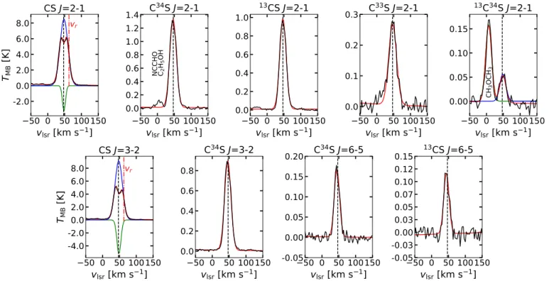
Fig. 2: From left to right and top to bottom: Observed line profiles of the J =2–1 transitions of CS, C34S,13CS, C33S, and 13C34S, the J =3–2 transitions of CS and C34S, and the J =6–5 transitions of C34S and 13CS, in the +50 km s−1Cloud
(EQ J2000: 17h45m50.20s, −28◦590
41.100). Measured profiles are shown in black; the resulting Gaussian fitting is presented in red. For the CS J =2–1 and J =3–2 lines, a double Gaussian fitting was performed to account for the self-absorbed component (in green) in an attempt to retrieve the undisturbed emission line (in blue) (see Sect.4.1). All the other lines are well fitted by a single component. In the case of 13C34S J =2–1, the companion line is subtracted because of its
relatively strong emission and potential contamination. The dashed vertical lines denote the13CS J =2–1 peak position
(46.94 km s−1, see Table2). Dash-dotted red lines denote the redshifted velocity (vr=63 km s−1) at which the CS J =2–1
and J =3–2 transition lines are not affected by self-absorption (see Sect.4.1). Nearby lines likely observed are labelled.
the topic of Sect.4.3. Generally, the analysis assumes that lines with the same rotational quantum numbers, related to different CS isotopologues, are co-spatial. We present a summary of our results in Table3.
4.1. Peak opacities and column density ratios in the +50 km s−1 Cloud
The CS emission lines observed towards the +50 km s−1Cloud are presented in Fig.2. All lines show peaks in agreement with the local standard of rest (LSR) velocity of the system, ∼50 km s−1 (Sandqvist et al. 2008; Requena-Torres et al. 2008). In addition to the CS J =2–1 isotopologue lines, there are probably weak features of cyanoformaldehyde (NCCHO) and ethanol (C2H5OH)
at 96.4260958 GHz and 96.4273380 GHz, respectively, on the blue-shifted side (∼0 km s−1) of C34S; dimethyl ether (CH3OCH3) at 90.9375080 GHz or ∼10 km s−1 on the
blue-shifted side dominates the 13C34S spectrum. Those molecules have been observed already in Sgr B2 ( Zucker-man et al. 1975; Nummelin et al. 1998; Martín-Pintado et al. 2001;Remijan et al. 2008;Belloche et al. 2013).
Moreover, the CS J =2–1 and J =3–2 line profiles show double-peaked profiles, which are readily explained by self-absorption, centred at the systemic velocity of the cloud in the J =2–1 transition and with a self-absorption marginally redshifted (by ∼0.4 km s−1) in the J =3–2 transition. The
CS parameters allowed to vary freely and obtained from single- or double-component Gaussian fitting are sum-marised in Table2. They were obtained using a series of Python codes, mainly within the lmfit package4.
As can be seen in Fig.2, for the CS J =2–1 and J =3–2 lines, we have fitted a double Gaussian considering a posi-tive (in blue) and a negaposi-tive (in green) Gaussian component each. Their parameters are summarised in Table2, where the uncertainties were taken directly from the lmfit package (for details see AppendixD).
Given that CS J = 2–1 and J = 3–2 show double-peaked profiles, while the rare isotopologues exhibit a single peak in between, the CS lines are likely optically thick. This was also suggested by Tsuboi et al. (1999) who find that CS J = 1–0 is moderately optically thick in this object, with an opacity (τ ) of around 2.8. Then, we can further assume as a first approximation that C34S J = 2–1 is optically thin
in the expected case that 32S/34S 3 (see Sect.4.1.2 for
a confirmation of this assumption; see alsoFrerking et al.
(1980) andCorby et al.(2018)). In this case13C34S J = 2–1
is definitively optically thin.
In the following we consider an excitation temperature range of 9.4–300 K for our column density computations in order to obtain conservative estimates. Our column density values were calculated using Eq. 80 in Mangum & Shirley
(2015) assuming a filling factor of unity. We then deduce
4
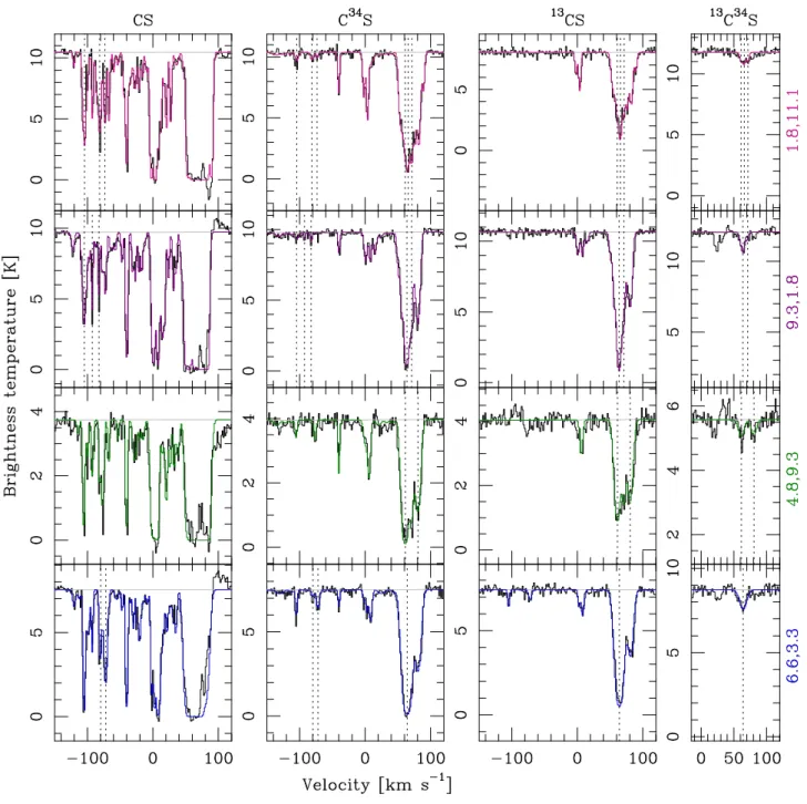
Fig. 3: EMoCA absorption spectra of four isotopologues of CS towards four positions in Sgr B2(N). The offsets (in units of arcseconds, see Table4and Fig.1) from the phase centre are indicated at the right of each row. The observed spectra are shown in black and the synthetic spectra in magenta, purple, green, and blue, depending on the position. The synthetic spectra were obtained by Thiel (2019). The dotted vertical lines indicate the velocities at which we determined the isotopic ratios using the corresponding isotopologue. The velocities are listed in Table4. The grey horizontal lines show the continuum level.
from the integrated line intensities of C34S J =2–1 and 13C34S J =2–1, converted to column densities, a 12C/13C
ratio of 22.1+3.3−2.4. This value is used in Equations 1 and2
(denoted RC), and it agrees with previous observations in
the GC within the uncertainties (∼17-25; e.g.Frerking et al. 1980;Corby et al. 2018), and with the values derived from many transitions of complex organic molecules (COMs) in the hot core Sgr B2(N2) (Belloche et al. 2016;Müller et al. 2016), indicating that our approach is correct and confirm-ing that C34S is indeed optically thin.
Assuming equal excitation temperatures (see Ap-pendixB) and beam filling factors for 12CS and13CS, the
13CS J =2–1 peak opacity τ (13CS) can then be determined
from TMB(12CS) TMB(13CS) =1 − e −τ (13CS)R C 1 − e−τ (13CS) , RC= 12C 13C. (1)
However, as there is a self-absorption feature at the centre of the12CS J =2–1 and J =3–2 profiles, we measure the line
temperatures of both12CS and13CS at a redshifted veloc-ity, vr= 63 km s−1, where the line shape is not affected by
self-absorption. We can then retrieve the opacity at the sys-temic velocity, assumed to be the13CS J =2–1 peak velocity, vsys=46.94 km s−1, by considering a Gaussian distribution.
First, we compute the opacities at vrin the following way:
TMB(12CSvr) TMB(13CSvr) =1 − e −τ (13CS vr)RC 1 − e−τ (13CS vr) , RC= 12C 13C, (2) 4.26 ± 0.11 0.24 ± 0.11 = 1 − e−22.1+3.3−2.4τ (13CSvr) 1 − e−τ (13CS vr) . (3) Here TMB(12CSvr) and TMB( 13CS
vr) are the
main-beam brightness temperatures of CS and 13CS J =2–1 at
vr. This results in τ (13CSvr) = 0.02±0.01, considering the
same uncertainties for the peak temperatures as those ob-tained by performing a single Gaussian fit in those lines. We can now retrieve the opacity at the systemic velocity as
τ (13CSvsys) =
τ (13CS vr)
e−(vr−vsys)2/2σ2, (4)
where σ is the full width at half maximum (FWHM) of 13CSvsys divided by p8ln(2) (FHWM/p8ln(2) =
9.46±0.12 km s−1) and vsys=46.942±0.118 km s−1. We
ob-tain τ (13CSvsys) = 0.08 +0.05 −0.04. Multiplying this by RC, we obtain τ (13CS vsys)RC= τ (CSvsys)=1.9 +1.1 −0.8, consistent with
previous observations (τ (CSvsys) ∼2.8;Tsuboi et al. 1999).
The uncertainty on vsys corresponds to a 0.15% variation
in the τ (CSvsys) value in the worst case. Therefore, it is
ignored in the following.
4.1.1. A32S/34S ratio obtained through the double isotope
method
As we have seen, CS must be moderately optically thick. Then, the32S/34S isotope ratios cannot be determined from the observed N (12CS)/N (C34S) ratio. Instead, we can use
the column densities of 13CS and C34S by realistically as-suming that those lines are optically thin (see Sect.4.1). Therefore, we have derived the values for 32S/34S making
use of the carbon isotope ratio mentioned above, in the following way: 32S 34S = 12C 13C N (13CS) N (C34S). (5)
From Eq.5 we obtain a 32S/34S J =2–1 ratio of 16.3+3.0 −2.4.
By using the13CS and C34S J =6–5 transitions, we obtain a 32S/34S J =6–5 ratio of 15.8+4.2
−3.4. This agreement within the
uncertainties can be taken as another argument in favour of the low opacity of C34S and the subsequent validity of
our assumptions and calculations. If some of the C34S lines in the rotational ladder were not optically thin, we would expect different N (13CS)/N (C34S) ratios in the J =2–1 and 6–5 transitions due to photon trapping leading to higher ex-citation temperatures in the more abundant isotopologue, which is not observed.
4.1.2.32S/34S ratio from direct observations
As we have measured the13C34S J =2–1 transition, we can
also obtain the32S/34S ratio directly from 32S
34S =
N (13CS)
N (13C34S). (6)
Using this we obtain a32S/34S J =2–1 ratio of 16.3+2.1 −1.7,
con-sistent with the ratio obtained through the double-isotope method in Eq.5 and again indicating that our initial as-sumptions concerning line saturation were correct. In the following, we use the latter value for our analysis because it was determined in the most direct way. In order to estimate the opacity of CS from C34S (see Sect.4.1.3), we use this C32S/C34S J =2–1 ratio of 16.3+2.1
−1.7 as the sulphur isotopic
ratio32S/34S and call it R S.
To compare our results with those ofChin et al.(1996), we also derived a sulphur ratio from the integrated intensi-ties:32S/34S ∼ I(13CS)/I(13C34S). This results in a32S/34S
value of 18.6+2.2−1.8. The differences between the column den-sity and integrated intenden-sity ratios are due to the rota-tional partition functions, rotarota-tional constants, and Ein-stein A-coefficients for spontaneous emission of radiation that slightly differ for the different isotopologues.
4.1.3. CS and C34S J=3–2 opacities
Now we are able to determine the opacities of CS and C34S J =3–2 by proceeding in the same way as in Equations 2
and 4, but considering this time the sulphur ratio. Here, as in Equation2, we also assume equal excitation temper-atures (see AppendixB) and beam filling factors, this time for12CS and C34S J =3–2: TMB(12CSvr) TMB(C34Svr) = 1 − e −τ (C34S vr)RS 1 − e−τ (C34Svr) , RS= 32S 34S. (7) From Eq.7, τ (C34S
vr)=0.01–0.03. Following the formalism
in Eq.4, we obtain a τ (C34S
vsys) value of 0.05–0.15.
En-tering this value and replacing τ (C34S
vsys)RS by τ (CSvsys),
the CSvsys opacity results in a proper range of 1.0–2.8,
con-sidering throughout this calculation that this latter value cannot lie below unity, since CS shows clear signs of opti-cal thickness (see Sect4.1). This is consistent with previous observations (Tsuboi et al. 1999). All the derived opacities are summarised in Table2.
4.1.4.34S/33S ratio from direct observations
The C33S J =2–1 line was also observed. This offers the
possibility of obtaining the34S/33S ratio for the GC. Since
C33S is less abundant than C34S, we can expect a clearly
optically thin profile. This ratio is easily obtained by
34S 33S =
N (C34S)
N (C33S). (8)
We obtain a 34S/33S ratio of 4.3±0.2 for the +50 km s−1Cloud. If we take the integrated intensi-ties instead of the column densiintensi-ties, this ratio would be 4.2±0.2, consistent with the lower end of the range of ratios obtained byChin et al.(1996), who derived34S/33S ratios between 4.38 and 7.53, irrespective of Galactic
radius. Whether this is a first hint of a gradient remains to be seen. Better data from the Galactic disc are necessary to tackle this question.
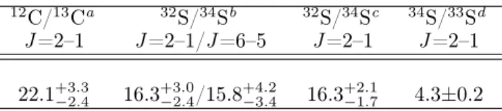
Table 3: Summary for our carbon and sulphur column den-sity ratio calculations in the +50 km s−1Cloud.
12C/13Ca 32S/34Sb 32S/34Sc 34S/33Sd
J =2–1 J =2–1/J =6–5 J =2–1 J =2–1 22.1+3.3−2.4 16.3+3.0−2.4/15.8+4.2−3.4 16.3+2.1−1.7 4.3±0.2
Notes.(a)From N (C34S)/N (13C34S) J =2–1 lines, as described in Sect.4.1.(b)Through the double isotope method in Sect.4.1.1. (c)
From direct observations in Sect.4.1.2.(d)Sect.4.1.4.
4.2. Modelling the Sgr B2(N) data
Here we rely on the modelling of the absorption profiles of the isotopologues of CS carried out by Thiel (2019) using the EMoCA survey, following the same method as Thiel et al. (2019). They used the software Weeds (Maret et al. 2011) to model the absorption profiles. Their work assumes that all transitions of a molecule have the same excitation temperature and that the beam filling factor is unity, which is a reasonable assumption given that most absorption fea-tures are extended on scales of 1500or beyond in the ALMA maps (seeThiel et al. 2019, their Sect. 5.4), while the beam size is 100. 6 (see Sect.2.2, Fig.1, and Table1). The fitted
parameters were the column density, line width, and the centroid velocity, under the assumption that the excitation temperature is equal to the temperature of the cosmic mi-crowave background (2.73 K).
We selected four continuum peaks inside Sgr B2(N) (Fig.1). We excluded the two strong continuum peaks at which the main hot cores N1 and N2 are located because at these positions the spectra are full of emission lines of organic molecules (e.g. Bonfand et al. 2017) contaminat-ing the carbon monosulfide absorption features. The offsets to the centre of the observed field are (100. 8, 1100. 1), (900. 3,
100. 8), (400. 8, 900. 3), and (600. 6, 300. 3) (see Fig.1and Table4). The
observed absorption profiles and the corresponding Weeds models for the four isotopologues and the four positions are shown in Fig.3. Using their results for the column densities, we determined the isotopic ratios CS/C34S, 13CS/13C34S,
and C34S/13C34S. We determined those ratios separately for the envelope of Sgr B2(N) and some GC clouds along the l.o.s. to Sgr B2(N), the latter with velocities lower than −50 km s−1. We only determine the ratio CS/C34S in those
cases where the absorption caused by CS is not optically thick.
The resulting unweighted average values of the isotopic ratios are listed in Table4, namely a32S/34S isotope ratio
of 16.3±3.8 in the GC l.o.s. clouds towards Sgr B2(N) and 17.9±5.0 in the envelope of Sgr B2(N). For this envelope we obtain a12C/13C ratio of 27.6±6.5. It should be noted that our uncertainties correspond to the standard deviation for independent measurements, i.e. without dividing it by the square root of the number of studied spectral components.
4.3. Discussion on the validity of using C32S/C34S as a proxy
for32S/34S
Chin et al. (1996) estimated that sulphur fractionation is marginal for CS isotopic ratios. If the bulk of the CS emis-sion, which allows us to measure rare isotopes, arises from the densest parts of the molecular clouds only, the heating from the massive stars should inhibit significant fractiona-tion (Chin et al. 1996). In that case, CS emission can be used directly to determine sulphur isotope ratios from such sources.
In their oxygen fractionation study,Loison et al.(2019) analyse sulphur fractionation including CS. Some sulphur fractionation is induced at low temperature by the 34S+
+ CS → S+ + C34S reaction. To determine the potential fractionation of sulphur, we used the network from Loi-son et al. (2019) in the +50 km s−1Cloud, the l.o.s. clouds
towards Sgr B2(N) and the envelope of Sgr B2(N), with re-alistic physical conditions for these objects, in particular a much higher value of the cosmic-ray ionisation rate (CRIR) than the usual value in more local dense molecular clouds. Some typical results are shown in Fig.4 and are described below.
In the simulations all elements with an ionisation po-tential below the maximum energy of ambient UV photons (13.6 eV) are assumed to be initially in an atomic, singly ionised state. We considered all sulphur in the S+ form without depletion, and we performed some tests to quantify the effect of depletion, which is low (see below). Hydrogen, with its high degree of self-shielding, is taken to be entirely molecular. The initial abundances are similar to those in Table 1 of Hincelin et al. (2011), the C/O elemental ratio being equal to 0.7 in our study. We verified that the initial state of carbon and nitrogen (C+ versus CO and N versus
N2) have very little influence on sulphur fractionation (less
than 4% for the typical ages considered: 105−6 years). The estimation of the dense cloud ages is deduced from clouds with similar density (104 to a few 105cm−3) for which the age is given by the best agreement between calculations and observations for key species given by the so-called dis-tance of disagreement (Wakelam et al. 2006). By key species we mean species typically encountered in molecular clouds such as HCN, HNC, CN, CH, C2H, c–C3H, c–C3H2, CO, H2CO, CH3OH, NO, SO, CS, HCS+, and H2CS (see e.g. Wakelam et al. 2010; Agúndez & Wakelam 2013; Agúndez et al. 2019).
For Fig.4a, which represents conditions in the +50 km s−1Cloud, we adopted a density of 105cm−3and a
CRIR of ζH2 = 7×10⁻¹⁶s−1based on measurements in hot
cores of Sgr B2(N) by using COMs (Bonfand et al. 2019). For Fig.4b and c, which represent the conditions for the en-velope of Sgr B2(N) and the l.o.s. clouds towards Sgr B2(N), respectively, we chose a density of 104cm−3, an upper limit
for the volume density in those regions (see Thiel et al. 2019, their Table 12), in order to avoid possible UV heating in our models. Due to this high density, we have adopted a CRIR of ζH2 = 3×10⁻¹⁵s−1, i.e. one order of
magni-tude lower than the value usually obtained in the l.o.s. of translucent and diffuse clouds towards the Galactic centre, but within the range obtained for the nuclear ∼100 pc of our Galaxy (Indriolo et al. 2015;Le Petit et al. 2016). The
32S/34S isotope ratio chosen for each simulation is that
ob-tained from our measurements, namely 16.3+2.1−1.7, 17.9±5.0, and 16.3±3.8 for Figs.4a, b, and c, respectively.
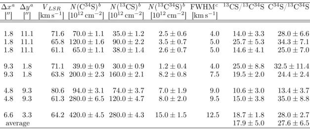
Table 4: Isotopic ratios determined in the envelope of Sgr B2(N) (13CS/13C34S and C34S/13C34S) and in GC clouds along the line of sight to Sgr B2(N) (CS/C34S) using absorption lines of CS isotopologues.
Isotopic ratios determined in the envelope of Sgr B2(N)
∆xa ∆ya V LSR N (C34S)b N (13CS)b N (13C34S)b FWHMc 13CS/13C34S C34S/13C34S [00] [00] [km s−1] [1012cm−2] [1012cm−2] [1012cm−2] [km s−1] 1.8 11.1 71.6 70.0 ± 1.1 35.0 ± 1.2 2.5 ± 0.6 4.0 14.0 ± 3.3 28.0 ± 6.6 1.8 11.1 65.8 120.0 ± 1.6 90.0 ± 2.2 3.5 ± 0.7 5.0 25.7 ± 5.3 34.3 ± 7.1 1.8 11.1 61.1 65.0 ± 1.1 38.0 ± 1.4 2.6 ± 0.7 5.0 14.6 ± 4.1 25.0 ± 7.0 9.3 1.8 71.1 39.0 ± 0.9 30.0 ± 0.9 1.2 ± 0.4 4.0 25.0 ± 8.8 32.5 ± 11.4 9.3 1.8 63.8 200.0 ± 2.3 160.0 ± 2.1 8.2 ± 0.8 7.5 19.5 ± 2.0 24.4 ± 2.4 4.8 9.3 80.6 94.0 ± 3.1 74.0 ± 3.7 7.0 ± 1.9 9.0 10.6 ± 3.0 13.4 ± 3.7 4.8 9.3 61.3 280.0 ± 6.5 120.0 ± 4.7 8.0 ± 2.0 9.5 15.0 ± 3.8 35.0 ± 8.8 6.6 3.3 64.2 420.0 ± 4.5 280.0 ± 4.3 15.0 ± 1.5 12.5 18.7 ± 1.8 28.0 ± 2.7 average 17.9 ± 5.0 27.6 ± 6.5
Isotopic ratios determined in GC clouds along the line of sight to Sgr B2(N)
∆xa ∆ya V LSR N (CS)b N (C34S)b FWHMc CS/C34S [00] [00] [km s−1] [1012cm−2] [1012cm−2] [km s−1] 1.8 11.1 -73.3 26.0 ± 0.7 1.4 ± 0.5 3.5 18.6 ± 6.3 1.8 11.1 -81.2 45.0 ± 0.9 2.5 ± 0.6 5.0 18.0 ± 4.0 1.8 11.1 -104.2 58.0 ± 1.0 3.0 ± 0.6 5.0 19.3 ± 3.6 9.3 1.8 -82.5 16.0 ± 0.7 1.4 ± 0.4 2.5 11.4 ± 3.7 9.3 1.8 -92.6 20.0 ± 0.7 1.2 ± 0.5 2.5 16.7 ± 7.3 9.3 1.8 -104.7 63.0 ± 1.1 3.0 ± 0.7 6.5 21.0 ± 4.9 6.6 3.3 -71.8 65.0 ± 1.5 7.2 ± 0.8 5.5 9.0 ± 1.0 6.6 3.3 -79.8 29.0 ± 1.0 1.8 ± 0.6 4.0 16.1 ± 5.8 average 16.3 ± 3.8
Notes.(a)The offset positions (∆x, ∆y) in units of arcseconds: (1.8, 11.1), (9.3, 1.8), (4.8,9.3), and (6.6, 3.3), correspond to K4, K6shell, K5shell, and K6shell,a, in Fig.1, respectively. See the caption to Fig.1and the green crosses in the image.(b)Column densities determined using Weeds.(c) It is assumed that all isotopologues have the same FWHM . The average isotope ratios presented by the lowest line of each panel are unweighted and provide the standard deviation of an individual measurement (without dividing by the square root of the number of ratios).
Despite the limited literature on the subject, according to models fromLaas & Caselli(2019), the +50 km s−1Cloud is the only object in this study that could show signs of sulphur depletion. However, for a depletion level of up to 90%, our models give results consistent with no sulphur de-pletion (which is the case for the results shown in Fig.4) because of the high temperatures that prevent any efficient fractionation. It should be noted that if this cloud’s chem-istry was determined in an earlier colder evolutionary pe-riod with possibly significant sulphur fractionation, CS, in contrast to CO, could not accumulate because it would have been destroyed by protonation as the dissociative recombi-nation of HCS+leads mainly to S + CH and not to CS + H (see AppendixA). Therefore, the memory effect for the CS fractionation of such a dense cloud is small. For the l.o.s. clouds towards Sgr B2(N) and the envelope of Sgr B2(N), some runs (those shown in Fig.4) give some sulphur frac-tionation when the gas temperature is low. This is due to the combination of low density limiting the depletion of
sul-phur and a high CRIR (ζH2 = 3×10⁻¹⁵s−1). These
char-acteristics induce an elevated concentration of S+ in the
gas phase and then a34S enrichment through the34S+ +
CS → S+ + C34S reaction (see Table 2 in Loison et al. 2019). It should be noted that the cases with some34S
en-richment only concern low kinetic temperatures, and that this relatively low enrichment will be even lower with some sulphur depletion. This depletion is not well constrained in the +50 km s−1Cloud, the l.o.s. clouds towards Sgr B2(N), and the envelope of Sgr B2(N), but it is high for some cold dense molecular clouds (between 10 and 25 for the dark cloud L1544 Barnard 1b (Fuente et al. 2016) and even up to 200 for the dark cloud L1544 (Vastel et al. 2018).
The extremely low gas temperature cases in our models (black lines in Fig.4) are shown to demonstrate the de-pendence of sulphur depletion on gas temperature. Since Galactic centre molecular cloud temperatures are higher (Ginsburg et al. 2016), CS shows likely very little fraction-ation in34S for the purposes of this study and our
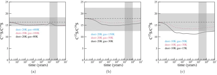
measure-dust=20K gas=80K dust=20K gas=100K dust=20K gas=400K 1 101 102 103 104 105 106 107 0 5 10 15 20 25 C 32 S /C 34 S time (years) (a) dust=20K gas=30K dust=20K gas=50K dust=20K gas=150K 1 101 102 103 104 105 106 107 0 5 10 15 20 25 C 32 S /C 34 S time (years) (b) dust=10K gas=15K dust=10K gas=30K dust=10K gas=50K 1 101 102 103 104 105 106 107 0 5 10 15 20 25 C 32 S /C 34 S time (years) (c)
Fig. 4: Calculated abundance ratios of gas phase species C32S/C34S as a function of cloud age for conditions in (a) the
+50 km s−1Cloud, (b) the envelope of Sgr B2(N), and (c) l.o.s. clouds towards Sgr B2(N) (see Sect.4.2for details). Low values for the gas temperatures were chosen to illustrate an upper limit for fractionation. The vertical grey loci represent values given by the most probable chemical age. The observational results from this study are illustrated as horizontal light grey rectangles (including the uncertainties).
ments of the C32S/C34S ratio are a good approximation to
the 32S/34S ratio (even if the values thus obtained may
be slightly underestimated when considering the results of the models). We can then expect a .10% increase in the
32S/34S ratios obtained for the +50 km s−1Cloud in Fig.4a
and slightly more for the l.o.s. clouds towards Sgr B(N) and its envelope (.15%), considering the conditions labelled in red and blue in Figs.4b and c.
Some measurements using the double-isotope ratio method (see Sect.4.1.1), which take the12C/13C ratio into
account, may induce a bias since CS may show a non-negligible fractionation into13C. There is no specific study of the 13C fractionation of CS, but the reactivity of C+
and C, in particular with CO and CN (but also with CS), can induce an enrichment or depletion in 13C of
carbona-ceous species including CS (Smith & Adams 1980; Roueff et al. 2015). In that case, the good agreement between the sulphur fractionation measurements using C32S/C34S and
the values obtained using the double-isotope method also suggests a low13C fractionation of CS. This result is
inter-esting and could initiate future studies on the modelling of
13C fractionation in CS.
5. Our results in the light of previous studies
If we assume that the gradient proposed by Chin et al.
(1996) would also be valid in the Galactic centre region, the 32S/34S ratio would decrease to values of 4.1±3.1 at
the centre of our Galaxy, i.e. to a very low value, only 1/4 of the solar system ratio. This value is less than one fourth of the value derived from integrated intensities in this work, 18.6+2.2−1.8.
This difference can be explained in terms of the12C/13C
ratios assumed in Chin et al. (1996), required to obtain the 32S/34S ratio through the double-isotope method by using the formalism of Eq.5(although using intensities in-stead of column densities). The 12C/13C ratios were de-rived from the relation found byWilson & Rood(1994) of
12C/13C = (7.5 ± 1.9)(D
GC/kpc) + (7.6 ± 12.9) that gives
a value of 7.6+12.9−7.6 for the Galactic centre, although the
authors claimed a value of ∼20 near the Galactic nucleus (Wilson & Rood 1994, Sect 5.1). This provides an idea of the large uncertainty in this relation.
On the other hand, we are confident about our12C/13C ratio of 22.1+3.3−2.4(Sect.4.1) for two reasons: first, the agree-ment between the 32S/34S ratio obtained through the
double-isotope method (Sect.4.1.1), which makes use of the
12C/13C ratio, and the32S/34S ratio obtained directly from 13CS/13C34S (Sect.4.1.2), i.e. independently of the carbon
ratio (this also indicates that the carbon fractionation is low, as described in Sect.4.3) and second, its proximity to the ratio obtained through decades of observations in the nuclear regions of our Galaxy (12C/13C = 17–25, Frerking et al. 1980;Wilson & Rood 1994;Milam et al. 2005;Müller et al. 2008; Corby et al. 2018), including LTE modelling of complex organic molecules (Belloche et al. 2016; Müller et al. 2016). There is no abrupt redirection in the12C/13C ratio (e.g.Henkel et al. 1985).
Recently, Corby et al. (2018) found 32S/34S ratios
mostly in the 5–10 range, based on C32S and C34S J =1–0
absorption lines from diffuse clouds near the GC, with a resolution of ∼1500. Considering their data in the –73 to – 106 km s−1 velocity range, corresponding to our GC l.o.s. clouds towards Sgr B2(N), their observations reach values between 6.6±6 and 29±14, consistent with our values be-tween 9.0±1.0 and 21.0±4.9 (Table4, lower panel).
In addition,Armijos-Abendaño et al.(2015), with a res-olution of ∼3000–3800, found values of &22 and 8.7±1.3 for
32S/34S isotope ratios in l.o.s. clouds towards Sgr A and
Sgr B2, respectively, consistent with previous estimations (Frerking et al. 1980). However, their sulphur ratios were obtained from OCS/OC34S, with OCS being potentially
op-tically thick and OC34S spectra being badly affected by band pass ripples, possibly providing only tentative detec-tions. So we propose a more conservative lower limit for the l.o.s. clouds towards Sgr A of ∼10 and we suggest that the uncertainty for their ratio in Sgr B2 was underestimated.
Both Corby et al.(2018) and Armijos-Abendaño et al.
(2015) employed integrated column density ratios, so we should compare those measurements with our normal
32S/34S isotope ratio estimation, that is 16.3+2.1
−1.7 for the
+50 km s−1 Cloud (as an approximation for their l.o.s. clouds towards Sgr A) and 16.3±3.8 for the l.o.s. clouds towards Sgr B2 (see Table4). Our data represent a signifi-cant improvement in terms of accuracy and precision with respect to those previous observations. In addition, our es-timation of 17.9±5.0 for the envelope of Sgr B2(N) agrees with both estimations for the +50 km s−1 Cloud and also with previous calculations for the whole Sgr B2 region: ∼16, from the OCS/OC34S ratio, which is claimed to be derived from optically thin lines (Goldsmith & Linke 1981).
Cutting-edge model calculations performed by
Kobayashi et al. (2011) relate sulphur isotope ratios (32S/33,34,36S) with metallicity ([Fe/H]5). We can use this relation in combination with a given metallicity gradient along the Milky Way ([Fe/H] versus DGC/kpc), to derive a 32S/34S versus D
GC/kpc relation and compare it with our
measurements.
Table 3 of Kobayashi et al. (2011) gives values for the 32S/34S ratio as a function of [Fe/H] over the range
–0.5≤[Fe/H]≤0.0. We can derive the following relation by interpolating their data:
32S
34S = −19.8 × [Fe/H] + 23.2. (9)
Extrapolating up to [Fe/H]≤0.85, we can account for the inner part of our Galaxy. Then, to relate 32S/34S to the galactocentric distance, we can make use of the relations obtained by Bovy et al. (2014) and Genovali et al.(2014), valid for 5≤DGC/kpc≤14–19, respectively:
[Fe/H] = (−0.09 ± 0.01) × (DGC/kpc − 8) + 0.03 ± 0.01, (10)
[Fe/H] = (−0.06 ± 0.002) × DGC/kpc + 0.57 ± 0.02, (11)
and combine them with Eq.9, to obtain the following rela-tions:
32S
34S = (1.8 ∓ 0.2) × (DGC− 8 kpc) + 22.6 ∓ 0.2, (12)
32S
34S = (1.2 ∓ 0.04) × DGC+ 11.9 ∓ 0.4. (13)
Equations (12) and (13) are plotted in Fig.5 as hatched-shaded regions. As described in the legend, their extrapo-lations down to 2.53 kpc, following Inno et al.(2019, their Figure 11), for both Eqs.10and11, are indicated as hatched regions only.
Additionally, we have accounted for iron abundances ob-tained from high-resolution near-infrared observations by
Davies et al. (2009) and Najarro et al.(2009) in the inner 30 pc of the Galaxy (see alsoKovtyukh et al. 2019). Their measurements are [Fe/H]=0.1±0.2 and −0.06±0.2, respec-tively, and we converted them to 32S/34S ratios of 21.2±4
and 24.4±4 by applying Eq.9.
In summary, the relations of both Bovy et al. (2014) andGenovali et al.(2014), through Eq.9, give results closer to those obtained from the double-isotope method (Eq.5),
5
where [Fe/H] = log10([NFe/NH])star- log10([NFe/NH])sun
considering12C/13C ratios byYan et al.(2019) in
combina-tion with the13C32S/C34S ratios fromChin et al.(1996), as can be seen in Fig.5(dotted blue line). In the nuclear region of the Galaxy the Davies et al. (2009) and Najarro et al.
(2009) observations, when accounting for Eq.9, are both consistent with our measurements for the +50 km s−1Cloud and the envelope of Sgr B2(N).
6. Discussion
Among the four stable sulphur isotopes (32S,33S,34S, and 36S), 32S is a primary nucleus which could be synthesised
in a single generation of massive stars.32S is mostly formed
during stages of hydrostatic and explosive oxygen-burning (Wilson & Matteucci 1992) either preceding a Type II su-pernova event or in a Type Ia susu-pernova, where two 16O
nuclei collide to form28Si and4He, with these products sub-sequently fusing to yield32S. Type II supernovae synthesise
around ten times more 32S than Type I supernovae, and occur roughly 5 times as often as those of Type I (Hughes et al. 2008). 33S is partly a secondary isotope because it can be formed by neutron capture from newly made32S if
the star not only has hydrogen and helium, but also car-bon and oxygen in its initial composition (Clayton 2007). It is synthesised in hydrostatic and explosive oxygen- and neon-burning, also produced in massive stars.34S is partly a secondary product because it can be formed from newly made32S and33S by neutron capture, but also during oxy-gen burning in supernovae like the primary isotope, 32S
(Hughes et al. 2008, and references therein). While the com-prehensive calculations ofWoosley & Weaver (1995) iden-tify 32S as a primary isotope, the same study also found
that 34S is not a clean primary isotope; its yields decrease with decreasing metallicity. However, they identify33S as a
primary isotope, in contradiction with later findings ( Clay-ton 2007). 36S is probably the only purely secondary
sul-phur isotope, being produced by s-process nucleosynthesis in massive stars (Thielemann & Arnett 1985;Mauersberger et al. 1996) and also by explosive C and He burning and via direct neutron capture from 34S, according to models (Pignatari et al. 2016).36S could be the only S isotope not
only produced from massive stars but also, to a lesser ex-tent, from AGB stars (Pignatari et al. 2016). However, lines from C36S are too weak to be detected in this study. Mas-sive stars, as well as Type Ib/c and II supernovae, appear to slightly overproduce34S and underproduce33S compared
to32S, relative to the solar vicinity (Timmes et al. 1995).
The main result of our study is that the previous trend observed byChin et al.(1996) is broken near the centre of our Galaxy. In other words, the increase in 32S/34S with
DGC is not valid in the Galactic centre region. The values
of 16.3+2.1−1.7 from the +50 km s−1 Cloud and 16.3±3.8 and 17.9±5.0 from the GC l.o.s. clouds towards Sgr B2(N) and its envelope, respectively, contrast with the expected ∼5– 10 regardless of the value of12C/13C adopted (see Fig.5)
when accounting for the 13C32S/C34S ratios used in Chin et al.(1996). It is also worth mentioning that our32S/34S
isotope ratios derived from absorption lines from diffuse or translucent clouds (Sgr B2(N)) are consistent with values derived from emission lines from a prominent star-forming region with dense molecular gas (the +50 km s−1Cloud), even though the chemistry for CS formation is completely different in those regions (see AppendixA).
0
2
4
6
8
D
GC[kpc]
0
10
20
30
40
50
32S/
34S
extrapolation following Inno et al. (2019) extrapolation following Inno et al. (2019) Najarro et al. (2009) + Kobayashi et al. (2011) from Genovali et al. (2014) + Kobayashi et al. (2011)
from Bovy et al. (2014) + Kobayashi et al. (2011) Davies et al. (2009) + Kobayashi et al. (2011)
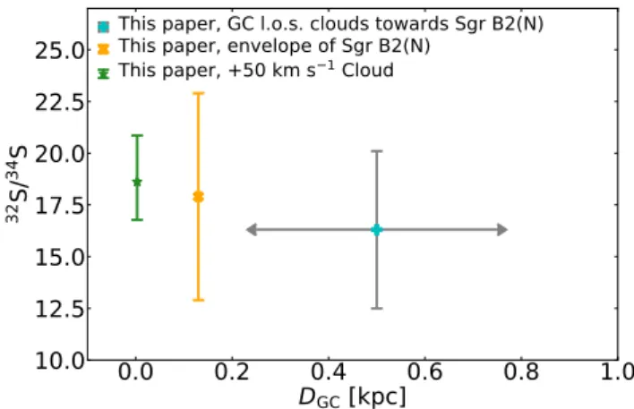
12C/13C from Wilson and Rood (1994) 32S/34S = (3.4±0.5)×DGC+ (3.9±3.1) 12C/13C from Milam et al. (2005) 32S/34S = (2.7±0.5)×DGC+ (9.4±3.1) 12C/13C from Halfen et al. (2017) 32S/34S = (2.2±0.5)×DGC+ (11.3±2.9) 12C/13C from Yan et al. (2019) 32S/34S = (2.2±0.4)×DGC+ (6.0±2.4)
This paper, GC l.o.s. clouds towards Sgr B2(N)
This paper, envelope of Sgr B2(N)
This paper, +50 km s
1Cloud
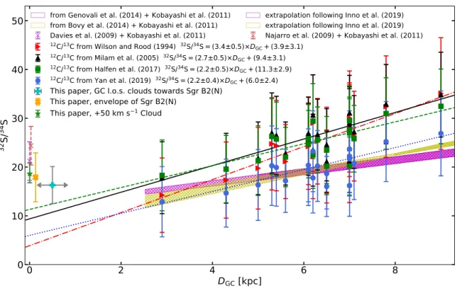
Fig. 5: Sulphur isotope 32S/34S ratio variation when accounting for different carbon 12C/13C ratios as a function of galactocentric radius, DGC (e.g. Wilson & Rood 1994; Halfen et al. 2017; Milam et al. 2005; Yan et al. 2019) (for the
implemented 13C32S/C34S ratios, see Chin et al. 1996). The 32S/34S to DGC relations obtained from a linear
least-squares fit to weighted data (taken as 1/σ, see Sect.5) are shown and plotted as lines with different styles (see legend). The 32S/34S ratios from this work are shown in orange, cyan, and light green. All ratios were gleaned from integrated
intensity ratios except for Sgr B2(N) (see Fig.3), where our derived integrated column density ratios are used. Possible differences between integrated column density ratios and line intensity ratios for the mean values in Sgr B2(N) fall inside the error bars. For the case of the GC l.o.s. clouds towards Sgr B2(N), their distances are uncertain and they are believed to be located within 1 kpc from the GC (see Sect.3). As described in Sect.5, the purple and yellow hatched-shaded loci are derived from [Fe/H] vs DGCrelations obtained byBovy et al.(2014) andGenovali et al.(2014), after accounting for
the models ofKobayashi et al.(2011); hatched-only loci correspond to an extrapolation of those relations, followingInno et al. (2019). Using the same models, two32S/34S ratios are included. These ratios are derived from iron abundances measured in the central 30 pc of the Galaxy byDavies et al. (2009) andNajarro et al. (2009). A zoom on the results of our study displayed in the left part of the figure is shown in Fig.C.1.
Frerking et al.(1980), even before the32S/34S slope was
found, suggested values for32S/34S of ∼22 for the Galactic centre. Therefore, the sulphur ratio seems to be constant, or even increases with decreasing DGC, within the inner
2.9 kpc of the Milky Way, in contrast to12C/13C (e.g.Yan et al. 2019), 14N/15N (e.g. Adande & Ziurys 2012), and 18O/17O (Wouterloot et al. 2008; Zhang et al. 2015).
In-triguingly, 32S/34S behaves in a similar way to 16O/18O
(Polehampton et al. 2005), two nuclei with the bulk of their formation taking place in massive stars (≥10 M ) (Clayton 2007). This is surprising because34S is a tracer of secondary processing as 13C and 15N, and therefore its abundance is
expected to increase in the same manner as observed for those isotopes.
The fact that sulphur traces late evolutionary stages of massive stars can give a clue to this difference in comparison to C and N, which give information on CNO and helium burning (Chin et al. 1996). Due to their short lives, the
star formation rate of massive stars can be traced by their SN rate. Although the amount of 34S is related to metal-licity, which decreases with increasing galactocentric radius especially in spiral galaxies (e.g. as observed from oxygen,
Henry & Worthey 1999), leading to a trend similar to C and N, the production of34S is mostly related to SNe II, which
show a dip in the inner regions of our Galaxy and other spiral galaxies (Anderson & James 2009), in good agree-ment with our higher than expected 32S/34S ratios in the Galactic centre. However, these results are still under de-bate (see e.g.Hakobyan et al. 2009) and more observations are needed.
Another argument in favour of the above could be that metallicities traced by iron (Genovali et al. 2014;Kovtyukh et al. 2019) instead of oxygen (Henry & Worthey 1999) show a trend in good agreement with our observations (after converting [Fe/H] to DGC/kpc not only outside the central