HAL Id: hal-01711436
https://hal.archives-ouvertes.fr/hal-01711436
Submitted on 24 Oct 2019
HAL is a multi-disciplinary open access
archive for the deposit and dissemination of
sci-entific research documents, whether they are
pub-lished or not. The documents may come from
teaching and research institutions in France or
abroad, or from public or private research centers.
L’archive ouverte pluridisciplinaire HAL, est
destinée au dépôt et à la diffusion de documents
scientifiques de niveau recherche, publiés ou non,
émanant des établissements d’enseignement et de
recherche français ou étrangers, des laboratoires
publics ou privés.
Heliospheric interstellar H temperature from
SOHO/SWAN H cell data
Jorge Costa, Rosine Lallement, Eric Quémerais, Jean-Loup Bertaux, Erkki
Kyrölä, Walter Schmidt
To cite this version:
Jorge Costa, Rosine Lallement, Eric Quémerais, Jean-Loup Bertaux, Erkki Kyrölä, et al.. Heliospheric
interstellar H temperature from SOHO/SWAN H cell data. Astronomy and Astrophysics - A&A, EDP
Sciences, 1999, 349 (2), pp.660-672. �hal-01711436�
AND
ASTROPHYSICS
Heliospheric interstellar H temperature
from SOHO/SWAN H cell data
J. Costa1, R. Lallement1, E. Qu´emerais1, J.-L. Bertaux1, E. Kyr¨ol¨a2, and W. Schmidt2 1 Service d’A´eronomie du CNRS, Verri`eres le Buisson, France ([email protected])
2 Finnish Meteorological Institute, P.O. Box 503, FIN-00101 Helsinki, Finland Received 5 May 1999 / Accepted 4 June 1999
Abstract. We show a first comparison between selected
SOHO/SWAN H cell data recorded in 1996–1997 and a simple classical “hot model” of the interstellar (IS) H flow in the inner heliosphere. Our goal is to obtain some constraints on the inter-planetary background Ly-α profiles, for the first time without any assumption on the H cell characteristics. For this purpose the H cell optical thickness and its temperature are free parame-ters of the study, but we assume that the direction of the flow and the allowed range for the upwind line-of-sight apparent Doppler shift are known from previous studies.
We derive apparent temperatures (or line-of-sight (LOS) temperatures) between 11,000 and 20,000 K according to the direction. This implies a significant broadening with respect to the linewidths expected for a flow at the same temperature as the interstellar helium flow (6,000± 1000 K) in the optically thin approximation. Radiative transfer is probably responsible for a fraction of this effect, and heating at the heliospheric interface for the remaining. The best solutions are found for an upwind velocity of 26 km s−1, in excellent agreement with an indepen-dent study by Qu´emerais et al. (1999), and for very similar H cell absorption width and temporal decrease. The deceleration of interstellar H at heliopause crossing is found to be between 2.5 and 4.5 km s−1.
We also use one particular H cell absorption map to derive directly from the data how the LOS temperature (or linewidth) varies with the angle with the wind direction. Interestingly, we measure a temperature minimum between the upwind and crosswind directions, while classical models predict a monotonic increase of the LOS temperature from upwind to downwind. We believe that this behavior is the first evidence for the existence of two distinct populations at different velocities (primary and secondary IS atoms), as predicted by heliosphere-interstellar gas interface models. If confirmed, this should be an extremely good diagnostic of the interface.
Key words: Sun: solar wind – inteplanetary medium – ISM:
general
Send offprint requests to: J. Costa
1. Introduction
The Sun is moving through the Local Interstellar Cloud (LIC) at a velocity of the order of 26 km s−1(Lallement & Bertin, 1992, Bertin et al., 1993). The solar wind builds a cavity, the helio-sphere, within the ionized gas component of the LIC (for recent developments see Von Steiger et al., 1996). On the contrary, neutral atoms of the LIC enter the heliosphere where they can be observed by remote sensing of resonance scattering of solar lines (121.6 nm for H (Lyman-alpha or Lα) and 58.4 nm for He). Helium atoms and neutral derivatives as pick-up ions and cosmic rays have also been detected “in situ”, but not hydro-gen atoms. The helium flow properties are now well constrained from a series of measurements (M¨obius, 1996, Witte et al., 1996, Gloeckler, 1996, Flynn et al., 1998) which result in a common interval for the bulk velocity and the temperature V(He)= 25.5± 0.5 km s−1and T(He)= 5000–7000 K. These velocity and tem-perature are in agreement with the velocity and the temtem-perature of the LIC deduced from stellar spectroscopy (Lallement et al., 1995, Linsky et al., 1995), as expected for helium which is sup-posed to enter freely the heliospheric cavity. At variance with helium, hydrogen is expected to be perturbed by coupling with the decelerated plasma via charge-exchange (e.g. Izmodenov et al., 1999). Neutral hydrogen heating and deceleration thus pro-vide a measurement of this coupling and in turn of the plasma density in the local interstellar medium which is responsible for most of the confinement of the heliosphere. One of the objec-tives of the SWAN (Solar Wind Anisotropies) experiment on board SOHO is the determination of the H flow characteristics precisely enough to measure departures from the helium flow and infer the deceleration and heating of H at the heliopause due to charge-exchange interaction. Recently Qu´emerais et al. (1999) have done a model-independent study of a first year of SWAN data. The present work is conducted in parallel and is complementary, as we will see below. Ideally, the analysis of the SWAN data should be done with the use of a unified model including many second order effects as the solar wind and radi-ation anisotropies (e.g. Kyr¨ol¨a et al., 1998), time dependence of the solar parameters (e.g. Rucinski & Bzowski, 1996, Bzowski et al., 1997), heliospheric interface modifications (e.g. Bara-nov & Malama, 1993, Williams et al., 1997, IzmodeBara-nov et al., 1999), and radiative transfer. These effects have been studied
es-sentially separately but each refinement requires large amounts of computer time. This, plus the huge amount of data to study, explains why we start with a simplified model in order to get a zero degree solution in a preliminary phase. Before summariz-ing the results obtained to this date for hydrogen, we first recall some definitions.
Hereafter what we call “temperature” of the flow or temper-ature “at infinity” T0is the maxwellian temperature of the gas just before it begins to suffer perturbations by solar gravity, su-personic wind and radiation, i.e. at a distance of about 50 A.U. for hydrogen, and 20 A.U. for helium. This means inside the heliosphere, after the gas has flown through the heliospheric in-terface. For helium, which keeps the characteristics it had in the interstellar medium, T0is identical to the interstellar tempera-ture TLIC, and the assumption of a maxwellian flow is valid. For hydrogen, the velocity pattern is influenced by the heliospheric interface, T0 >TLIC and the velocity distribution of the flow “at infinity” may depart from a pure maxwellian. Nevertheless, in this paper which presents a first approach we still assume that we can represent the flow as it comes out from the interface by a maxwellian flow with a bulk velocity V0and a temperature T0, that we attempt to retrieve from a comparison of a forward model to SWAN data.
On the other hand, what we call “apparent” temperature of the H Ly-α emission or “line-of-sight (LOS) temperature” in a given direction of sight is simply the line-width of the Lyα emis-sion from this direction, interpreted in terms of a maxwellian profile (See Fig. 1). The emission is the integrated light from the observer up to large solar distances where the emissivity be-comes negligible. In other words, LOS temperatures reflect the local velocity distribution (by local we mean in the inner helio-sphere), weighted by the solar illumination (variable along the LOS) and averaged along the LOS. The reason we are mainly interested in LOS temperatures is that they are the only measur-able quantity in terms of spectroscopy, and thus we are forced to model it.
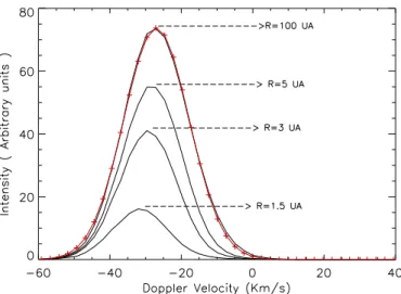
The LOS temperature differs significantly from the temper-ature at infinity T0for two main reasons: (i) gravitation, radia-tion pressure and selecradia-tion of particles during the ionizaradia-tion pro-cesses modify the velocity distribution, and (ii) radiative transfer of Lyα light modifies the line profiles. The broadening actu-ally connected to the modification of the velocity distribution is shown in Fig. 1, which displays the line profile as calculated by the model when integrated from the earth orbit up to 100 A.U. The main effect is the increase of the flow bulk velocity when approaching the Sun, even when radiation pressure balances gravitation (µ=1), due to a longer lifetime against ionization of the fast particles. The figure shows the particular case of the upwind direction, but the phenomenon is similar in other direc-tions. According to the classical hot models, which start with a maxwellian flow and calculate its evolution in the inner helio-sphere under the action of supersonic solar wind, and solar ra-diation and gravitation (e.g. Lallement et al., 1985, see Sect. 3), the velocity distribution broadening is increasing from upwind (from where comes the flow) to downwind (the opposite direc-tion) and varies between 0 (upwind) and 35–80% (downwind),
Fig. 1. Example of building up of an emission line profile during the
integration along the line-of-sight. The profile is computed for an ob-server located at 1 A.U. on the crosswind side and looking towards the upwind direction. The emission originating in the closest regions has a higher Doppler shift, even in caseµ=1, due to selection of fast particles. The curve marked with plus signs is a maxwellian fit to the 100 AU integrated emission.The apparent temperature or LOS temper-ature is associated with the linewidth of this fitted maxwellian profile. Parameters are those from model 3.
depending on the location of the spacecraft and the model pa-rameters. This broadening is thus by definition precisely taken into account in the classical modeling. The broadening con-nected with radiative transfer, however is only very partially taken into account in the model we use here (see Sect. 3).
Time dependence of the solar wind properties and solar ra-diation have been studied and shown to introduce some depar-tures from the stationary case in terms of intensity (Rucinski & Bzowski, 1996, Bzowski et al., 1997). However, we do not expect very important effect in terms of bulk velocity and tem-perature changes. At variance with such effects, the influence of the solar line shape is mainly on the bulk velocity (Scherer et al., 1999).Variations of the order of up to 2 km s−1are to be considered. However, we have kept a flat solar profile for the following reason: the self-reversal of the line is responsible for a preferential illumination of the faster atoms. On the upwind side, this will result in a stronger blueshift of the line. On the other hand, those atoms which are better emitters are also those which suffer the strongest radiation pressure and thus are more repulsed. This repulsive effect acts in an opposite way when compared to the line shape effect. Only models taking into ac-count velocity dependent radiation pressure can really acac-count for the whole phenomenon. This is beyond the scope of this paper which deals with first-order effects first. However, this deserves further modelling, especially full time-dependent and velocity-dependent models.
Two types of spectroscopic tools have been applied up to now to the measurement of the H resonance glow line profile at Lα, hydrogen cell absorption and direct spectroscopy of the interplanetary glow. In the case of a H cell (see next Sect. 2 for its principle), the profile retrieval is not direct. Depending on
the quantity and geometry of data, more or less assumptions are necessary. The Prognoz data analysis (Bertaux et al., 1985) led to V0= 20± 1 km s−1 and T0=8000± 1000 K, assuming the temperature in the cell was Tc= 300 K, i.e. the experiment temperature, and the optical thickness in the range of 8–10. Due to this assumption, the parameters V0and T0were not totally independently derived, but there was no reason at this time to question the H cell parameters. There was also a specificity of the Prognoz experiment: there were no mechanisms allowing to vary the line-of-sight, and only the earth motion along its orbit and the spin of the spacecraft around the Earth-Sun line could be used to probe different directions. Due to this restricted geometry, regions of the sky probed by the cell (i.e. with actual absorption by the cell) were all perpendicular to the flow and at high ecliptic latitudes (where the LOS is perpendicular to both the Earth’s and the wind velocities).
Direct spectroscopy provides the line width of the emission without any assumption. Spectra of the H Ly-α glow recorded with the HST-GHRS have been obtained by Clarke et al. (1998), who report apparent temperatures as high as 17000 K± 4000 K and 30000 K± 15000 K respectively for the upwind and down-wind directions in 1995, which implies a temperature T0 signifi-cantly above the 8,000 K deduced from Prognoz H cell data. On the other hand, they report Tapp=9000 K (± 2000 K) in 1994 for the crosswind side (or perpendicularly to the flow), i.e. a range compatible with T0 =8,000 K. They argue that such a pattern may be satisfyingly explained by preferential broadening along the wind axis as predicted by interface models when there is a very strong coupling with the plasma (Lallement et al., 1992). But the required electron density later appeared too strong to really match the filtration or interstellar measurements (Lalle-ment, 1996). The HST results have also been compared with line profiles resulting from models including an interface (Scherer et al., 1997,99). In this case, the input parameter is the temperature outside the heliosphere, in the unperturbed interstellar medium. Since interface models of any kind predict a heating of the gas, these model temperatures can be chosen much smaller than the temperature of the flow in the inner heliosphere, the departure between the two temperatures being strongly dependent on the assumed electron density in the surrounding ISM. As an ex-ample, for plasma densities of 0.10–0.14 cm−3, those used by Scherer et al. (1999), the heating predicted in the 2-shocks case is of the order of 6000–8000 K (Izmodenov et al., 1999), i.e. of the same order as the initial temperature itself (of the order of 7000 K). Here our goal is to obtain from the data an estimate of the temperature inside the heliosphere, independently of any assumption on the interface. The results will serve later as a diagnostic of the interface all along with the improvements of interface models.
The H cell is presently the unique technique to provide spectroscopic diagnostics over the full sky, especially because high resolution spectrometers in space do not have a large enough etendue (S xω) to allow measurements within a rea-sonably small time, and their spectra recorded from low alti-tude orbits are strongly contaminated by the geocorona, which
is not the case at the SOHO location (L1 Lagrange point at 1,500,000 km s).
On the other hand, a careful analysis of laboratory measure-ments performed during the preparation of the SWAN project has recently shown that for optical thicknessesτ of the order of 10, the H gas produced in the cell may be heated above 300 K and that absorption equivalent widths could have been underes-timated when interpreting the calibration measurements of the H cell parameters. This is why we have undertaken the present study and use SWAN data for a data-model comparison with-out assumptions on the H cell characteristics. The price to pay being a large computer time, our goal here is restricted to the determination of a velocity-temperature range for the H flow, and not a full multi-parameter fit to the data.
HST direct spectroscopy provided a measurement of the Doppler shift of the emission profile. On the upwind side the Doppler shift represents the velocity distribution of the ap-proaching gas weighted by the solar illumination. It was found to be 23 (resp. 21.5 and 23.5) km s−1in 1992 (resp. 1994 and 1995), with uncertainties of the order of 1 km s−1. In the frame of classical models these shifts were estimated to correspond to a bulk velocity at infinity V0 of 20± 1 km s−1 (resp. 18 and 21 ± 2 km s−1) (Lallement et al., 1993, Clarke et al., 1998). These velocities being substantially smaller than the helium flow velocity, such results were interpreted as a sign for the deceleration of H at the interface. However, it is important to note that the emission from the upwind side originates mainly within the first 2 or 3 A.U. from the Sun, i.e. where the gas is illuminated and still not totally ionized. At such distances, ve-locity changes induced by the combination of gravitation and radiation pressure play an important role. For this reason, the relationship between the measured upwind Doppler shift and the initial velocity (before solar influence) does depend on the Lα radiation pressure modulus, classically expressed by µ, the ratio between the radiation pressure force and the gravitational force. The recent UARS-SOLSTICE measurements of the so-lar H Ly-α radiation favor a stronger intensity (and a stronger
µ) in comparison with previous data (De Toma et al., 1997).
While the Prognoz analysis suggested µ= 0.75 at solar cycle minimum activity, in agreement with integrated solar disc Lα SME data, SOLSTICE on UARS predictsµ= 1.0 for the same period. This uncertainty onµ introduces an uncertainty on V0 and thus on the deceleration. This is why a precise measurement of the heating, in addition to the deceleration, would be an im-portant improvement. In what follows, we will use the fact that the Doppler shifts themselves (and only the Doppler shifts) are directly obtained from the HST-GHRS spectra and do not suffer other uncertainties than the error bars on the measurements.
Very recently, and independently of the present study, Qu´emerais et al. (1999) have used an entire year of SWAN H cell data and performed a deconvolution using absorptions by the cell in the same direction at different periods of the year, which means for different Doppler shifts between the observer and the gas flow (see Fig. 3). They have provided a measure-ment of the L-O-S Doppler shift and linewidth for all direc-tions. This method is model-independent and does not use any
Model 3 & T=10250 K Model 4 & T=12850 K UPWIND DOWNWIND C,D A B
SIDEWIND (Through cavity) SIDEWIND (Outside cavity)
E,F
H
G
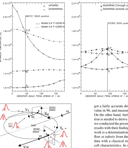
Fig. 2. Model apparent
tempera-tures or line-of-sight temperatempera-tures for 4 directions (upwind, downwind, sidewind) as a function of the loca-tion of the observer along the earth orbit. Models 3 and 4 are shown
V0 Vrel V0 V0 Vs Vs Vrel SUN ZDSC 3 2 plane ZDSC plane 1 Ly-a light a
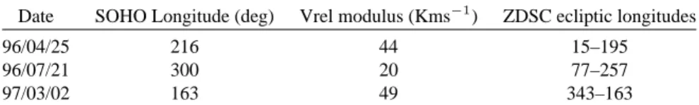
Fig. 3. Locations of SOHO along its orbit for the 3 maps and
approx-imate geometries for the wind, SOHO, and relative velocity vectors. Also drawn are the corresponding approximate Zero Doppler Shift Cir-cle planes for locations 2 and 3. Emission lines from line-of-sight in or close to the plane are strongly absorbed by the cell, i.e. the cell absorbs in the middle of the line. L-O-S at increasing angles from the ZDSC plane correspond to increasing Doppler shift and then smaller absorp-tion. Due to gravitation and selection of particles, the loci of maximum H cell absorption actually depart from planes, and this geometry is also slightly modified by the non-zero inclination of the flow with respect to the ecliptic plane.
assumption on the cell, but assumes that the emission profile from one particular direction does not vary when the observer moves along the earth (or SOHO) orbit. Models show that this is not true (see Fig. 2), especially on the crosswind (perpendic-ularly to the flow) and downwind sides, where corrections have to be done. On the upwind side this approach is justified. This is why the upwind Doppler shift of 25.4± 1 km s−1measured by Qu´emerais et al. (1999) in 1996–1997 is a very precise and unbiased measurement which can be directly compared with the above HST results as discussed in Sect. 3. These authors also
got a fairly accurate determination of the cell equivalent width value in 96, and measured its temporal variation in 1996–1997. On the other hand, further works to remove stellar contamina-tion is needed to derive l-o-s temperatures, which explains why we conducted the present study in parallel. We will compare our results with their findings. As said above, the goal of the present work is a determination of an interval for the temperature of the flow at infinity from the comparison of a selected set of SWAN data with a classical model, withoutany assumption on the H cell characteristics. In order to keep a reasonable computation time, we have made some symplifying assumptions which are based on the 3 following results deduced from previous obser-vations and analyses: (i) the direction of the flow is now well constrained, from Helium flow measurements and LIC absorp-tion spectroscopy towards nearby stars. (ii) the mean moabsorp-tion of the gas close to the Sun (measured by the upwind Doppler shift) is now constrained within an interval of a few km s−1from the different observations we have quoted above. (iii) the ionisation rate can be kept fixed in the study, since we are concerned with the H cell data, i.e. velocity distribution only. As a matter of fact, it has a noticeable influence on the density distribution and resulting Lα intensity pattern, but a much smaller one on the LOS line shapes.
In Sect. 2, data and geometry are described. Sect. 3 gives a brief description of the hot model used for the data/model comparison. Sect. 4 describes in detail the method we are ap-plying in the data analysis. In Sect. 5, we present the results of the data-model comparison and compare with some of the conclusions of Qu´emerais et al. (1999). In Sect. 6, we use the results of Sect. 4 and show a model-independent determination of the LOS temperature along a great circle. Sect. 7 discusses the different results.
2. H cell data
The SWAN experiment has been described in details in Bertaux et al. (1995). SWAN has provided full-sky maps of the H Lα glow every two days since Dec 1995 up to this date, thanks to two sensors symmetrically located on the spacecraft. The maps are used to measure the solar wind in three dimensions, the first objective of SWAN (Kyr¨ol¨a et al., 1998). On the other hand, the use of the H cell allows us to measure the velocity distribution of H atoms in the heliosphere. Data have been shown by Bertaux et al. (1997), Qu´emerais et al. (1999), Lallement (1999).
2.1. The H cell
Each SWAN sensor is equipped with a hydrogen absorption cell in the light path to the detectors which is alternatively acti-vated or deactiacti-vated. When the cell is ON, atomic H is produced from the dissociation of molecular H2, and the incoming light is absorbed by a column-density N of cold atomic hydrogen characterized by a temperature Tc and an optical thicknessτc = 5.9×10⁻¹²N T0.5c at line center. Photons are scattered away from the light path to the walls of the cell where they are ab-sorbed. All H cell measurements are obtained by comparing the counting rate when the cell is OFF (Ioff = total intensity) and the cell is ON (Ion = transmitted intensity), for the same line of sight. If I(λ) is the emission line profile, the transmission profile isT (λ, τc, Tc) defined by Eq. (1)
T (λ, τc, T c) = e−τce−x2 (1) wherex = λ−λ0 ∆λc ,∆λc = λ0 c q 2kT c mh = λ0Vc c is the H cell
thermal Doppler width,Vcis the thermal velocity of the atomic H in the cell andλ0is the Lymanα wavelength (1215.663 ˚A). We then have: Ioff = Z +∞ −∞ I(λ) dλ (2) Ion = Z +∞ −∞ I(λ)T (λ, τc, T c) dλ (3) R = IIon off = R+∞ −∞ I(λ)T (λ, τR c, T c) dλ ∞ −∞I(λ) dλ (4) The ratioR is called the transmission factor (it was also often called reduction factor in the past, although this term may be misleading), and is a function of the cell parametersTcandτc, and, for a given cell, of both the relative motion of the emitting gas and the absorbing gas of the cell along the line-of-sight (the Doppler shiftVD) and of the emission linewidth, i.e. the temperature of the emitting atoms. The absorption A by the cell is A= 1-R.
The equivalent widthWλ of the absorption line profile in the H cell is defined, as is classical, by:
Wλ= Z +∞
−∞ (1 − T (λ, τc, T c)) dλ
(5) It can be measured in wavelenght units or in km s−1. Since the thermal Doppler velocity spread inside the cell, where the
tem-perature is close to 300 K, is smaller than the thermal broadening of the interplanetary H line profile, where the temperature is of the order of 10000 K, the absorption line created by the cell (half-width 0.015 ˚A) is narrower than the interplanetary H line profile emission (half-width 0.07 ˚A) and only a fraction of the light is absorbed, even when the Doppler shift between the H cell (SOHO) and the interplanetary H is zero. When the Doppler shift is not zero, the H cell absorption is even smaller and may go to zero for higher values of Doppler shift. The H cell atoms do absorb the incoming photons when their wavelength in the frame of the cell falls within the thermal Doppler width of the cold gas.
2.2. Selected transmission maps
Fig. 3 shows the approximate geometry for the three trans-mission maps we have selected for the present study. On this simplified plot the interstellar wind motion is assumed to be maxwellian and constant everywhere and characterized by the vector −→Vo. The heliocentric orbital motion of SOHO (about 30 km s−1) is represented by the vector−→Vs. The absorption is at first order a function of the projection of the relative motion
−−→
Vrel = −V→o− −→Vsbetween the flow and the cell, onto the
line-of-sight. When the line of sight is along theVrelaxis, the cell absorption is shifted out from the center of the emission line and there is no (or a small) absorption for these directions. On the contrary, when the SWAN line of sight is perpendicular toVr, the emission line is not Doppler shifted for an observer linked to SWAN and the H cell atoms do absorb at the center of the emission line (see Fig. 3). Such a maximum absorption occurs close to the plane perpendicular to V−rel→intersecting the celes-tial sphere along a circle called the Zero Doppler Shift Circle (ZDSC) (Bertaux & Lallement,1984).
Table 1 gives the characteristics of the 3 configurations for the data maps which are schematized in Fig. 3. The three maps have been chosen because their respective ZDSC’s are oriented in specific ways. For maps 2 and 3 the angles between the ZDSC’s and the wind axis are close to 0◦ (along the axis: map 2), and 90◦(map3) respectively. Map 1 corresponds to and an intermediate value of about 30◦. Together the three ZDSC’s represent a good coverage of the sky. We have used for this par-ticular study the data of the North sensor only (the SU+Z), i.e. the one which operates at positive ecliptic latitudes, because the two H cells on the two sensors are different and have evolved with time in different ways, and the south sensor has a lower signal to noise ratio. Data points contaminated by starlight and straylight (solar and anti-solar directions) have been carefully removed from the data using a hot star catalog. About 50% of the data points are removed, leaving for each map about 18,500 pts. Coordinates are ecliptic.
2.3. Sensitivity of the ZDSC to velocity and temperature of the flow
The relationship between the relative velocity vector and the ZDSC angular width is an essential point and the basis of the
Table 1. Characteristics of the 3 transmission maps. The relative velocity modulus and the ecliptic longitudes at which the ZDSC crosses the
ecliptic plane has been estimated for V0=20 km s−1
Date SOHO Longitude (deg) Vrel modulus (Kms−1) ZDSC ecliptic longitudes
96/04/25 216 44 15–195
96/07/21 300 20 77–257
97/03/02 163 49 343–163
present data-model comparison. The larger (resp. smaller) the relative velocity modulus Vr, the smaller (resp. larger) the an-gle from the ZDSC center for which the H cell absorption line is shifted out from the emission line, for a constant Tapp(or emission linewidth), which is equivalent to a constant T0. If one wants to reproduce a given (measured) ZDSC angular width4α with different couples of values for Vrand T0, increasing (resp. decreasing) Vrrequires to increase (resp. decrease) T0. An ap-proximate relationship, valid for a gaussian homogeneous flow, is Vrsin(4α) ≈ (2kTmapp)1/2 (Bertaux & Lallement, 1984). Now, because the relative velocity Vris either decreasing or in-creasing with the gas velocity V0according to the location along the orbit (see Fig. 3), adjustingV0to fit transmission maps like map 2 (sidewind-right) and map 3 (sidewind-left) will influence on T0(and then on Tapp) in opposite ways for the 2 maps. This shows that the use of different parts of the orbit brings indepen-dent constraints on T0 and V0. Unless V0is well fitted, maps such as 2 and 3 will be fitted with different temperatures, which is unacceptable. We will see that this effect is conspicuous in our results.
3. The “hot” model
The model used in what follows is the so-called classical “hot” model (e.g. Lallement et al., 1985), which assumes a maxwellian flow far from the Sun, where it has not yet been modified by so-lar ionization, gravitation and radiation pressure (say, 50 A.U.). Here, it is applied to the H gas after it has been modified by the heliospheric interface. In other words this model represents the H flow in the inner heliosphere. It computes all individual atom trajectories under action of gravitation and radiation pres-sure (or the ratioµ), as well as the losses by ionization along each individual path. Note that this method differs from models in which dynamics and ionization losses are calculated inde-pendently, and which do not take into account some particular selection effects. For a given line-of-sight it computes the inte-grated emission profile using the resulting velocity distributions at each point along the L-O-S, and the classical scattering phase function. Here the solar line is assumed to be flat. The existence of a self reversal in the solar emission line modifies slightly the emission, but the effect on the linewidths is not expected to be significant.
Finally, self-absorption is included between the emitting volume and the observer, but not between the Sun and the emit-ting volume. In this respect, it differs from a full optically thin approximation, and it will yield some broadening of the lines. From our past experience it is the simplest way to take into
account radiative transfer (RT), when one is not using a full RT code, which is beyond the scope of this paper. For the den-sity at infinity we have chosen n0 = 0.125 cm−3. For such a density, the apparent temperatures are approximately 10–15% higher when we include self-absorption in this way by com-parison with the optically thin model, for the same T0. Due to the relationship between T0 and the LOS temperatures, T0 is model dependent, more specifically it strongly depends on the way radiative transfer is calculated. However, what we actually fit are the LOS temperatures. During the fitting procedure, T0 will be calculated in such a way LOS temperatures fit the data, whatever the relationship between them and T0. This is why we have to be cautious in drawing any conclusion based on the derived T0, but this is not the case if we draw conclusions on the basis of the LOS temperatures only.
4. Description of the method
used here for the data/model comparison
As said in the introduction, here we have used the fact that some quantities have been already very strongly constrained by pre-vious and also SWAN observations: - (i) the direction of the flow: we useλ = 254.5 and β = 7.5◦, as measured by Bertaux et al., (1985), and close to the values deduced from the retrieval of the velocity pattern of the SWAN data (Qu´emerais et al., 1999), which areλ = 253 and β = 8.5◦. This direction is also close (within 3◦) to the helium flow direction. (ii) the line-of-sight apparent velocity Vup in the direction of the incoming wind: as discussed in the introduction: this quantity has already been measured or inferred from a series of measurements. Di-rect observations with Copernicus, IUE, and HST have led to Vup= 21 to 24 km s−1(Adams & Frisch, 1977, Lallement et al., 1993, Clarke et al., 1984, 1995, 1998). Cell analyses led to 23± 1 km s−1(Bertaux et al., 1985) and to 25.4± 1 km s−1(SWAN, Qu´emerais et al., 1999). We believe that the somewhat high value measured by Swan in 96–97 is connected to solar mini-mum influence, resulting in a decrease of the radiation pressure after the 96 solar minimum (see the discussion).
Because the upwind apparent motion is governed by two parameters: the velocity far from the Sun V0and the radiation pressure (measured by µ), we then have selected four (V0
-µ) couples leading to line-of-sight velocities Vup between 22
and 26 km s−1. The 4 sets of parameters, hereafter referred as models 1 to 4, are listed in Table 2: these models thus predict a bulk velocity of the gas close to the Sun within the above limited range. The first model corresponds to an upwind appar-ent motion Vup of 22 km s−1, i.e. the lower range among the
Fig. 4. The north-ecliptic cell transmission
maps for the 3 locations of Fig. 3 (Location 1 on top, 2 in the middle, 3 at bottom). The maximum absorption regions for the three maps, when added, cover almost the entire North ecliptic sky.
Table 2. Characteristics of the 4 models and of the adjustment of the temperature T0, and the cell parameters Tcandτc. The upwind velocity is always larger than V0, even for straight trajectories (µ=1), due to preferential ionisation of the slowest particles.
Model V0km s−1 µ VUP km s−1 best fit T0K best fitτc best fit TcK
1 18 0.99 22 10,600-13,500 3.1-3.3 220-360
2 20 0.90 24.5 10,800-11,600 3.0-3.2 250-320
3 21 0.75 26 9,900-10,700 1.4-2.1 460-640
4 22.5 0.99 26 12,200-13,200 2.3-3.1 330-380
observations. The second corresponds to 24.4 km s−1, an inter-mediate value, and two V0-µ couples correspond to the high range, namely 26 km s−1, close to the SWAN Doppler shift of 25.5 km s−1 of Qu´emerais et al. (1999). The first from these two high Vupmodels corresponds to a small value ofµ(0.75), and thus to a correspondingly small V0(21 km s−1), while the second on the contrary is for a high value ofµ, in agreement with the recent SOLSTICE data, and a higher V0(22.5 km s−1). The last assumption is that we can at first order use any total ionization rateβ at 1 A.U. (equivalently any lifetime against ion-isation TD=β−1) within the most probable range TD=1.0–2.5 106s, because varying the ionisation rate changes very strongly the density, but has a small influence on the apparent velocity on the upwind side. We use TD=of 1.8×10⁶s (value at 1 A.U), an intermediate value between the expected low latitude high ionisation and the high latitude lower ionisation (Kyr¨ol¨a et al., 1998).
Apart from these assumptions, for the first time in such a study and data-model comparison, we do NOT assume any par-ticular value of the H cell parameters, i.e. we vary both the cell temperature and its optical thickness. This means that for a given (V0-µ) couple producing a reasonable upwind Doppler shift, we vary the temperature T0of the gas at infinity and for each T0we compute the model for all the directions of sight (about 18,500 points for each north ecliptic map), we then calculate the predicted cell transmission factor for a grid of cell parameters
τcand Tcand compare with data, until we get a minimum data-model discrepancy. For the adjustment we search for a minimum ofχ2=P(Rdata−Rmodel
Rdata )
2. This allows to derive the best com-bination of (T0,Tc andτc) for the full map. The full procedure is applied successively to the three H-cell transmission maps of Fig. 4. By doing so, we investigate the full range of reasonable values for all the parameters V0,µ, T0, Tc andτc. Also, we do not assume any rate of decrease of the H cell thickness,
Model 1 Model 2 Model 3 Model 4 96/04/25 96/07/21 97/03/02
Fig. 5. Residuals for the best-fit to
the data as a function of the flow temperature T0 at infinity, for the 4 models and the 3 maps. For comparison, the temperature T0 of the helium flow is smaller than 7,000 K. The use of an optically thin model would lead to temper-atures T0 between 10 and 15% higher than the plotted tempera-tures. LOS temperatures, which are the quantities really measured here, vary for the best models (mini-mumσf) between 10,000 (upwind) and 20,000 K (downwind). They are much higher than what the model would predict for a flow at T0=6,000
± 1,000 K, showing that a strong
broadening occurs.
cause this will be automatically taken into account by varying freely the cell parameters, independently for each map. We will check in finewhether the equivalent width Wλ of the cell has a temporal evolution compatible with the independent study of Qu´emerais et al., (1999).
5. Results
Fig. 5 showsσf =
q χ2
N, i.e the mean departure from the model
transmission factor as a function of the gas temperature T0for the 3 maps and the 4 models (i.e. the 4 couples (V0,µ) which lead to a reasonable upwind velocity). Each point is the best fit among all Tc and τc values.σf is to be compared with the average uncertainty on the measured transmission factorσd(determined in sky regions where the cell does not absorb) which is of the order of 0.010–0.012. Minimum valuesσsof 0.013 (resp. 0.020) correspond to data-model systematic discrepancies 30% (resp 100%) above the noise level.
Two types of conclusions can be drawn from these results. First, there are strong differences between the models from the point of view of the resulting best-fit temperatures derived for the 3 maps, which should be similar, if the model does repre-sent the data reasonably well. For example, model 1 (18 km s−1,
µ=0.99) is definitely inadequate. The high temperature (up to
14,000 K) derived from map 2 (July) and the much smaller tem-perature 10,000 K derived from map 1 (in March) are incon-sistent, a typical consequence of an underestimate of the flow velocity, an effect we have discussed in Sect. 2.3. As a matter of fact, in March (resp. July) the earth and the gas travel in op-posite (resp. same) directions, the modulus of Vris too small (resp. large), and subsequently the derived T0 too large (resp. small). This shows that a mean motion as small as 22 km s−1 is precluded by the data. On the contrary temperatures derived
from the 3 maps for models 2, 3 and 4, (Vup = 24.6, 26.5, 26.4 km s−1respectively) show much smaller variations of the minimum T0from map to map (∆ T0< 1,500 K), showing that the actual value of Vupat the time of the SWAN observations was within the high range (about 24.5–26.5 km s−1). A care-ful inspection of Fig. 5 shows that the temperature behaviour of model 2 is of the same type as for model 1 (although variations are much smaller), while model 4 shows (slightly) the opposite trend. Taken altogether these results show that the motion of the gas within a few A.U., represented by the upwind bulk motion, should be of the order of 25.5–26 km s−1. This is in very good agreement with the upwind apparent velocity of 25.5 km s−1 de-duced by Qu´emerais et al., (1999) independently of any model. This shows that our model velocity distributions can be used to represent the general behaviour of the flow, at least at first order. Model 1 has a small mean σf but a major default. Fig. 6 shows the best-fit H cell absorption equivalent widths Wλfor the 4 models as a function of time (i.e. the dates of the selected maps). We know from laboratory experiments and past expe-rience that a H cell absorption width slightly decreases with time when it is used regularly. Indeed, as quoted above it has been estimated from an independent SWAN data analysis that between mid-96 and mid-97 Wλof SU+Z sensor has decreased roughly by 10% (Qu´emerais et al., 1999). What is apparent from Fig. 6 is that for models 1 and 2 the equivalent width derived from the best fit H cell parameters does not decrease smoothly with time, but has a maximum for map2. This suggests that the model parameters and the derived cell parameters are not a good representation of the reality. More precisely, what happens is a consequence of what we have discussed above: because the tem-peratures deduced from the July map (2) are too high, due to the underestimated mean velocity, during the adjustment of the cell
Model 1
Model 2
Model 3
Model 4
(Quemerais et al,1999)
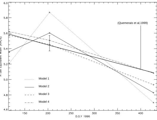
Fig. 6. The derived H cell absorption
line equivalent width (here in veloc-ity unit) for the 4 models. For mod-els 3 and 4 only, the temporal variation and the absolute values are fully consis-tent with the 10% decreased deduced by Qu´emerais et al. (1999).
parameters there is a compensation for the predicted too small absorption (the broader the emission linewidth, the smaller the absorption for moderate Dopplershifts), which forces the H cell equivalent width to a higher value. On the contrary, both models 3 and 4 correspond to a reasonable temporal evolution of the H cell absorption equivalent width, and at the same a small vari-ation of T0. In Fig. 6 is also represented the equivalent width estimated by Qu´emerais et al., (1999) from one year of SWAN data on the crosswind side, and the temporal evolution of this width. Taking into account the uncertainties on these estimates, the agreement with what is deduced from our adjustment in the case of models 3 and 4 is also very good (better than 5%). This shows that our best solution (in this context of a classical hot model) for parameters of models 3 and 4 is certainly close to the actual velocity distribution, because at the same time the H cell width, the H cell temporal evolution, and the mean motion Vup we derive from data/model comparison agree with the results of the model-independent analysis of Qu´emerais et al., (1999). The second conclusion we can draw is on the gas temper-ature. In the 4 cases, the best-fit temperature for the gas flow before the close interaction with the sun is always significantly higher than the temperature of the helium flow (or equivalently the local cloud temperature). From Fig. 5, the adjusted T0varies between 10,000 and 13,000 K. This is a consequence of the measured ZDSC’s width, depth, and location. Considering only adjusted models 3 and 4 which have the best cell characteristics and bulk motion, the temperature T0still varies between about 10,000 K, for the smaller value ofµ and then the smaller value of the velocity V0(= 21 km s−1), and 13,000 K for the larger
µ (=1) and the larger velocity V0 (= 22.5 km s−1). The small value of µ is the value deduced from Prognoz data analysis
and corresponds to the solar minimum case. In view of the new SOLSTICE data, this is certainly the smallest value we can rea-sonably consider here. The large value is of the order of what one would expect from the new SOLSTICE data. In the first case, the analysis implies a deceleration of about 4.5–5 km s−1 and a line broadening equivalent to a heating of 3,000 K. In the second case, the inferred deceleration is only 3–3.5 km s−1and the equivalent heating is as strong as 6,000 K!!. We can extrap-olate these results to possibly larger values ofµ. If the radiation pressure were larger thanµ = 1, we would find a larger V0in or-der to keep the same upwind Doppler shift, and we would infer a stronger heating and a smaller deceleration. In both cases, large departures from helium characteristics are certainly present.
One has to keep in mind however that the adjustment we are doing is the adjustment of the line-of-sight temperatures, which are what SWAN is actually measuring, and which we connect here through a model to the gas temperature at about 50 A.U. from the Sun. In other words, the value T0we deduce depends on the way we compute the intensity, i.e. it is model dependent. If the broadening of the lines due to radiative tranfer is stronger than what we take into account by including self-absorption between the L-O-S current point and the observer, then the temperature T0 we infer is overestimated, and on the contrary if a strictly optically thin model is actually the most appropriate, then the temperature T0we infer is underestimated by 5 to 15%. However, even if the modeled relationship between the LOS temperatures and T0is not correct, the LOS tempera-tures are still correctly estimated. We have checked this point by doing the same analysis in parallel with the presented calcula-tions with an optically thin model, for one map and one model. The adjusted temperature T0we have derived in this case was
Model 3 & T=10000 K Model 4 & T=13000 K
Fig. 7. Example of data-model
com-parison for the best-fit parameters for model 3 and 4. Here we show data and model as a function of ecliptic longitude atβ = 50◦for the 3 H cell transmission maps
indeed slightly higher (by 10% for n(H)=0.125 cm−3) than in the previous case, but the linewidths or LOS temperatures, now calculated in the optically thin frame were unchanged! This is why we focus now on the apparent temperatures predicted by the hot model.
The LOS temperatures for the upwind and downwind direc-tions Tupand Tdwand for the best models 3 and 4 have already been shown in Fig. 2-a as a function of the observer location along the earth orbit (for half an orbit). They were shown as an example of apparent temperature variation. Now, we use the figure for a better understanding of the best-fit results. For T0we have taken the average best-fit value for the 3 maps, i.e. 10,250 K for model 3 and 12,850 K for model 4. Fig. 2 shows that there is a particularly strong dependence on the earth longitude of the downwind temperature. As said in Sect. 2, this explains why the deconvolution of one year of SWAN data taken at all longitudes, under the assumption that the line profile does not depend on the location, requires some correction. Note that the tempera-ture variation is especially strong when the focusing is important (smallµ). In this case the downwind linewidth varies by almost a factor of 2 (model 3). In order to interpret the figure more precisely, it is necessary to recall that map 2 has been selected because its ZDSC plane is nearly parallel to the wind axis (i.e. the region probed by the cell contains the upwind and downwind directions). The longitude of SOHO for map 2 is at 45◦from the wind axis projection onto the ecliptic plane. Thus the UW and DW temperatures for model 3 (resp. 4) correspond to points A and C, (resp. B and D). It is interesting to note that C and D are very close, despite the strong difference of' 3,000 K in T0for the 2 models. The reason is that model 3 predicts a very strong line broadening on the downwind side (due to focusing) and
as a result a linewidth as large as for model 4 despite a much smaller T0. This explains why in our adjustment the use of a small µ forces T0 (and all l-o-s linewidths) to smaller values by comparison with the largeµ to get about the same down-wind linewidth. On the updown-wind side the two models predict a different temperature, because in all models the upwind tem-perature remains very similar to T0. The adjustment is a kind of compromise between the DW and UW sides. In any case, there is evidence that the DW linewidth corresponds to an apparent temperature of the order of 18,000 K, and the UW linewidth to 10,000–12,000 K.
Fig. 2-b is equivalent to 2-a, for the two sidewind directions. Note that despite the axisymmetry of the distributions along the wind axis, apparent temperatures towards the left and right sides are not the same and depend on the location of the observer being on the left or on the right. This is due to the fact that in one case the los crosses the cavity, in the other case not, and this has a strong influence on the line shape. This is essentially true when the focusing and filling of the cavity is strong (µ=0.75). The crosswind directions are probed in March, i.e. for map 3, i.e. for points E,F,G,H. Again it is interesting to see that for the sidewind direction through the cavity the two models predict the same width. We conclude that the data suggest an apparent temperature of the order of 12,000–15,000 K in the sidewind direction.
An example of data-model comparison is shown in Fig. 7 for the best-fit models 3 and 4 and a fraction of the data. We have selected three regions of the sky at low, medium and high ecliptic latitudes. The longitude varies between 0 and 360◦. The figure shows the quality of the adjustment, but also that there are systematic departures for both models (see next section).
22x103 20 18 16 14 12 10 8 Apparent temperature (K) 140 120 100 80 60 40 20
Angle with upwind (deg)
MAP 2 : 96-07-21 Model 3 Model 4
from absorption maxima
ß UPWIND CROSSWIND aaaa DOWNWIND
Fig. 8. Line-of-sight temperatures (Bars)
along the ZDSC of map2 deduced from the measured maximal absorptions and the al-lowed ranges for the cell equivalent width and temperature. Also represented are the l-o-s temperatures according to adjusted mod-els 3 and 4. There are significant differences in the pattern which are probably linked to heliospheric interface perturbations. We may see the crosswind “pinch” effect linked to the existence of two populations (primary and secondary atoms)
6. LOS temperature as a function of the angle with a wind axis
The most interesting map is certainly map2, because the maxi-mum absorption by the cell occurs over a wide range of angles with the upwind axis. We have derived the apparent temperature along the ZDSC of map2 in two different ways: -i) by using ad-justed models 3 and 4 -ii) independently of any model, by fitting the absorption hole across the ZDSC and deriving the minimum transmission factor Rmineverywhere along the circle, then sim-ply deducing from Rminthe maximum and minimum values for Tapp. This is done under the assumption that the emission is maxwellian, and that the H cell width and temperature are such that W = 5.37–5.57 km s−1(see the allowed interval in Fig. 6) and Tcvaries between 300 and 600 K. These ranges correspond to the results of Qu´emerais et al. (1999) (for W) and our present results (for W and Tc).
Resulting temperatures are shown in Fig. 8 and look partic-ularly interesting. Clearly the data and the models do not show the same type of variation of Rmin(and subsequently of Tapp) from the UW to the DW direction. More specifically, there is a minimum at about 50–60◦from UW in the case of the temper-ature directly deduced from the minimum of Rmin, while, as it is well known and can be seen in Fig. 8, the classical hot models predict a monotonic increase of Tapp. The observed behaviour could be related to the perturbations suffered at the heliospheric interface, and to the creation at this interface of two populations at different velocities, primary H atoms which have not suffered any charge-exchange with protons, and secondary H atoms re-sulting from charge-exchange between a decelerated interstellar proton and an interstellar H (e.g. Baranov and Malama, 1993, Izmodenov et al., 1999). This broadens the velocity distribu-tion width along the wind axis, while at 90◦from the axis, the two populations have both a very small Doppler shift and the broadening is minimal. The combination of the classical UW-DW monotonic increase of Tappplus the two-populations effect which increases Tapp preferentially UW and DW (or equiva-lently decreases Tapp on sidewind, something one could call a “pinch” effect) could certainly lead to the observed
behav-ior shown in Fig. 8. However, it remains that for this ZDSC crosswind directions are also high latitude directions. We do not preclude latitudinal anisotropies to be responsible for some deviations from the classical behavior and more work is needed in this direction.
Fig. 8 shows that the apparent temperatures deduced from the two methods are of the same order for the UW, CW and DW directions, i.e. 10,000–14,000, 13,000–15,000, and 17,000–20,000 K respectively for the three directions. This agreement on the mean level is expected because we have ad-justed the model in such a way the LOS temperatures fit the absorption data. The LOS temperatures are much higher than what one would expect for a flow at the temperature of helium (6000 K), implying a strong broadening. On the other hand, Fig. 8 also reveals in a conspicuous way the limitations of the hot model we have used. Differences between model and data are significant and require model refinements. In particular, the influence of the double flow, if confirmed, calls for a heliospheric interface model.
7. Discussion and conclusions
We have analyzed SWAN H cell absorption maps corresponding to 3 different locations of SOHO along the orbit. Starting with observational constraints on the mean motion of the gas derived from other analyses, we have searched for a best fit to the data with a classical hot model without any assumption on the H cell parameters.
The data/model comparison shows that the bulk motion of the gas observed on the upwind side is about 26 km s−1, in excellent agreement with Qu´emerais et al., 1999 who used a model-independent method. The comparison shows simultane-ously that, for those models which predict such an upwind mo-tion, the equivalent width of the cell and its temporal decrease (about 10% per year) are also extremely close to the model-independent results of Qu´emerais et al., 1999. These agreements show that the classical model can be used as a first order repre-sentation of the flow.
Because what is actually fitted during the temperature ad-justment is the ZDSC depth and width, the primary results are the LOS apparent temperatures. We derive them in two differ-ent ways. First, simply from the predictions of those models which have been adjusted to the data. Second, independently of the model, by using the measured absorption maxima along the ZDSC (when the cell absorbs in the middle of the emission line), and the equivalent widths we have derived (and found in agreement with Qu´emerais et al., 1999). As a matter of fact, as-suming the emission is maxwellian, one can derive from these two quantities its linewidth. We find from both methods LOS temperatures of 12,000± 2000, 14,000± 2000 and 18,500± 1500 K for directions at 20◦(close to upwind), 90◦(crosswind) and 150◦(close to downwind) respectively.
These values are in agreement with the recent HST measure-ments of very broad lines on the upwind and downwind sides (17,000 ± 4,000 K, 30,000 ± 15,000 K respectively, Clarke et al., 1998), but are above (by at least 1,000 K) the 9,000± 2,000 K derived for the crosswind region. Comparisons with previous H cell results are less direct. As we said, due to the geometry, the directions probed by the Prognoz experiment cor-responded to angles from the wind directions between 50 and 100 deg only and were all at high latitudes. Apparent tempera-tures deduced from the adjusted model were comprised between 9,000 and 10,000 K, also significantly below what we derive here for the crosswind side. We believe that the low Prognoz value is due to an underestimate of the H cell temperature and equivalent width. In the case of SWAN, thanks to the mapping of the full sky and the much larger amount of data it is possible to draw conclusions without any assumption on the H cell.
Independently of the general level of the temperatures, our study reveals that they do not increase in a monotonic way from the upwind to the downwind direction, as predicted by classical hot models, but are characterized by a minimum at about 50–60 deg from upwind. This suggests the existence of two flows at different velocities, as predicted by heliospheric interface mod-els, and should allow, if confirmed, excellent determinations of the coupling with the interstellar plasma, and of the interstel-lar plasma density (Lallement et al., 1992, 1995b). The order of magnitude of the deviation from the monotonic temperature pattern is about 3,000–6,000 K, as can be guessed from Fig. 8, which corresponds to a broadening of the line of 2 to 4 km s−1, i.e., of the same order as the mean deceleration we infer, when assuming a unique flow. However, we caution that more work is still needed to refine these line-profile results and disentan-gle double-flow characteristics from possible latitudinal effects linked with the solar wind anisotropies.
The flow temperature T0found from the model adjustment has a limited signification, because it is model dependent. Also, as said above, the LOS temperature pattern shown in Fig. 8 calls for a full model with heliospheric interface, in which T0includes a broadening due to the double flow. Nevertheless it gives an idea of the average heating-broadening. From our results T0 is comprised between 10,000 and 13,000 K, and represents the maxwellian temperature of the flow if there is negligible ra-diative transfer broadening. If not negligible, it is the sum of
the kinetic temperature plus a line broadening measured as a correction to the temperature. In any case, it is largely above the 5000–7000 K temperature of the helium flow, showing that the interface plus the radiative transfer (RT) of photons together very strongly broaden the H Ly-alpha line-profiles. According to Scherer et al. (1999), RT broadening should be negligible for l-o-s originating within the earth orbit al-o-s in our cal-o-se, leaving room for a strong heating of more than 3500 K at the heliospheric interface. It is also interesting to note that from the present data-model comparison it is impossible to distinguish between a strong broadening (heating) of at least 6500 K and a moderate deceleration of 2.5–3.5 km s−1(25.5 to 22–23 km s−1) in case of a large radiation pressureµ=1.0, and a stronger deceleration (25.5 to 21–22 km s−1) and a smaller broadening (heating) of 3500 K if there is a small radiation pressure (µ=0.75), or any intermediate situation. It still remains that there are significant perturbations with respect to the helium flow.
Work is in progress to model a larger amount of data, and to compare the above results with more sophisticated theoretical models of the flow, i.e. including radiative transfer and helio-spheric interface. It is however already extremely encouraging that SWAN apparently reveals some of the expected signatures of heliospheric interface impacts on the velocity distribution of H atoms, demonstrating its ability to constrain the characteris-tics of this interface.
Acknowledgements. The SOHO mission is a ESA/NASA international
cooperation. SWAN was financed in France by CNES with support from CNRS and in Finland by TEKES and the Finnish Meteorological institute. The data used in this work were obtained thanks to the help of the Experiment Operation and Flight Operation Teams at the Goddard Space Flight Center. Instrument operations were performed by Cyril Pennanech and Asko Lehto. We wish to thank Cyril Pennanech from Service d’ A´eronomie for his constant help with data processing and reduction, and Michel Berth´e and Jean-Pierre Goutail for all experi-mental aspects. We also thank Christian Bernard for the long-lived H cells of SWAN which have produced the above data.
We also thank our anonymous referee for having pointed out miss-ing explanations and discussions about the model assumptions.
References
Adams T.F., Frisch P.C., 1977, ApJ 212, 300
Baranov V.B., Malama Y.G., 1993, Journal of Geophysical Research 98, 15157
Bertaux J.L., Blamont J.E., 1971, A&A 11, 200
Bertaux J.L., Lallement R., Kurt V.G., Mironova E.N., 1985, A&A 150, 1
Bertaux J.L., Lallement R., 1984, A&A 140,230 Bertaux J.L., et al., 1995, Solar Physics 162, 403
Bertaux J.L., Quemerais E., Lallement R., et al., 1997, Solar Physics 175, 737
Bertin P., Lallement R., Ferlet R., Vidal-Madjar A., 1993, JGR 15193 Bzowski M., Fahr H.J., Rucinski D., Scherer H., A&A 1997, 326, 396 Clarke J.T., Bowyer S., Fahr H.J., Lay G., 1984, A&A 139, 389 Clarke J.T., Lallement R., Bertaux J.L., Qu´emerais E., 1995, ApJ 448,
893
Clarke J.T., Lallement R., Bertaux J.L., et al., 1998, ApJ 499, 482 De Toma J., Qu´emerais E., Sandel B.R., 1997, ApJ 491, 980
Flynn B., Vallerga J., Dalaudier F., Gladstone G.R., 1998, JGR 103, 6483
Gloeckler G., 1996, Space Sci. Rev. 78, 335
Izmodenov V.V., Geiss J., Lallement R., et al., 1999, JGR 104, A3, 4731
Kyr¨ol¨a E., Summanen T., Schmidt W., et al., 1998, JGR 103, A7, 14523 Lallement R., Malama Y.G., Qu´emerais E., Bertaux J.L., Zaitsev N.A.,
1992, ApJ 396, 696
Lallement R., Bertaux J. L., Dalaudier F., 1985, A&A 150, 21 Lallement R., Bertin P., 1992, A&A 266, 479
Lallement R., Bertaux J.L., Clarke J.T., 1993, Sci 21 Lallement R., 1996, Space Sci. Rev. 78, 1–2, 361
Lallement R., SWAN team, 1999, Solar Wind 9, Nantucket, Sept. 99, in press
Linsky J.L., Diplas A., Wood B.E., et al., 1995, ApJ 451, 335 Mobius E., 1996, Space Sci. Rev. 78, 375
Qu´emerais E., Bertaux J.L., 1993, A&A 277, 283
Qu´emerais E., Bertaux J.L., Lallement R., et al., 1999, JGR, in press Rucinski D., Bzowski M., 1996, Space Sci. Rev. 78, 265
Scherer H., Fahr H.J., Clarke J.T., 1997, A&A 325, 745
Scherer H., Bzowski M., Fahr H.J., Rucinski D., 1999, A&A 342, 601 Von Steiger R., Lallement R., Lee M. (eds.), 1996, The heliosphere in the Local Interstellar Cloud. Space Science Series of ISSI, Kluwer Academic Publishers (also Space Sci. Rev. 78, 1–2)
Williams L.L., Hall D.T., Pauls H.L., Zank G.P., 1997, ApJ 476, 366 Witte M., Banaszkiewicz M., Rosenbauer H., 1996, Space Sci. Rev.