HAL Id: hal-01276852
https://hal.univ-lorraine.fr/hal-01276852
Submitted on 26 Apr 2017
HAL is a multi-disciplinary open access
archive for the deposit and dissemination of
sci-entific research documents, whether they are
pub-lished or not. The documents may come from
teaching and research institutions in France or
abroad, or from public or private research centers.
L’archive ouverte pluridisciplinaire HAL, est
destinée au dépôt et à la diffusion de documents
scientifiques de niveau recherche, publiés ou non,
émanant des établissements d’enseignement et de
recherche français ou étrangers, des laboratoires
publics ou privés.
Distributed under a Creative Commons Attribution - ShareAlike| 4.0 International
License
Nicolas Cherpeau, Guillaume Caumon
To cite this version:
Nicolas Cherpeau, Guillaume Caumon. Stochastic structural modelling in sparse data situations.
Petroleum Geoscience, Geological Society, 2015, 21 (4), pp.233-247. �10.1144/petgeo2013-030�.
�hal-01276852�
Stochastic structural modelling in sparse data situations
Nicolas Cherpeau1, 2, Guillaume Caumon*11 Georessources (UMR 7566), Université Lorraine – ENSG / CNRS rue du Doyen Marcel Roubault, F-54518 Vandœuvre-lès-Nancy, France 2 Now with Paradigm, 78 Avenue du Vingtième Corps, 54000, Nancy, France.
* Corresponding author (email: [email protected])
Keywords: structural uncertainty; stochastic modelling; Abstract
This paper introduces a stochastic structural modelling method which honours interpretations of both faults and stratigraphic horizons on maps and cross-sections in conjunction with ancillary prior information such as fault orientation and statistical size-displacement relationships. The generated stochastic models sample not only geometric uncertainty but also topological uncertainty about the fault network. Faults are simulated sequentially; at each step, fault traces are randomly chosen to constrain a fault surface so as to obtain consistent fault geome-try and displacement profile. For each simulated fault network, stratigraphic modelling is performed to honour interpreted horizons using an implicit approach. Geometrical uncertainty on stratigraphic horizons can then be simulated by adding a correlated random noise to the stratigraphic scalar field. This strategy automatically main-tains the continuity between faults and horizons.
The method is applied to a Middle East field where stochastic structural models are generated from interpreted 2D seismic lines, first by representing only stratigraphic uncertainty and then by adding uncertainty about the fault network. These two scenarios are compared in terms of gross rock volume uncertainty (GRV) and show a significant increase of GRV uncertainty when fault uncertainties are considered. This underlines the key role of faults on resource estimation uncertainties and advocates a more systematic fault uncertainty consideration in subsurface studies, especially in settings in which data are sparse.
Introduction
Structural uncertainty is often a major but neglected factor in subsurface studies. Structural uncertainty typi-cally stems from the lack of observations or ambiguities of measurement and associated processing (e.g. limited resolution, lack of impedance contrasts, velocity uncer-tainty in seismic reflection data). In such a context, geo-logical interpretation is very important and relies on regional knowledge about the tectonic and sedimentary evolution of the area through time, in addition to physical laws describing rock behaviour. However, the interpreta-tion of seismic data may lead to various interpretainterpreta-tions by experts (Bond et al. 2007). Consequently, a given subsurface model should not be considered as the truth but as a possible representation of the subsurface honour-ing available information at a given stage. Additional data may then be used to update or even falsify the model in case of inconsistency with new data (Tarantola 2006). To address this challenge, several authors have proposed generating a set of possible structural models honouring subsurface data, then to use inverse methods to reduce uncertainty based on potential field or reservoir produc-tion data (Guillen et al. 2008; Suzuki et al. 2008; Seiler
et al. 2010; Jessell et al. 2010; Wellmann et al. 2010;
Aydin et al. (2014); Irving et al. 2014; Lindsay et al. 2014). The first stage in such approaches is to appropri-ately sample prior structural uncertainty. Most techniques (Lecour et al. 2001; Thore et al. 2002; Caumon et al. 2007; Mallet & Tertois 2010) start from an initial inter-pretation and perturb the geometry of the structures, but keep the topology frozen, i.e., do not change fault net-work connectivity. More recently, it has been proposed to perturb orientation data, which may have some impact
on the model topology (Jessell et al. 2010; Wellmann et
al. 2010; Lindsay et al. 2014; Wellmann et al. 2014). In
this paper, we propose a method which does not rely on an initial fault network interpretation, which removes possible interpretation bias carried by the initial model. In addition, it allows, in principle, to observe a larger variability in the simulated models because extrapolation away from the data is not constrained by some initial 3D model.
The Havana modelling tool introduced by Hollund et al. (2002) and Holden et al. (2003) similarly enables to generate fault networks which may have different topol-ogies. Originally, it simulated relatively small faults and the associated displacement along the pillars of a refer-ence reservoir grid (Rivenæs et al. 2005). More recently, Georgsen et al. (2012) and Røe et al. (2014) have pro-posed a more flexible data model based on tilted 2D grids and Gaussian random fields; faults are defined within fixed fault envelopes and intersections are man-aged by a cookie cutter strategy, which allows for topo-logical changes in areas where fault envelopes overlap. These approaches are suitable to represent uncertainty about fault locations on good 3D seismic data sets, but tend to only explore the uncertainty around a given struc-tural scenario.
In this paper, we focus on fault uncertainties in settings where the number and overall topology of faults is poorly constrained. This may typically occur in onshore explo-ration settings, or when 3D seismic acquisition or imag-ing is challengimag-ing, for example in deep and subsalt reser-voirs and in high-relief onshore areas. In these contexts, many different scenarios can be envisioned about the 3D fault network and the associated reservoir geometry and
connectivity. Exploring these scenarios with classical interpretation methods is demanding, costly, and subject to interpretive bias (Bond et al. 2007). Therefore, the goal of our method is to help interpretation tasks by au-tomatically generating alternative models of field geome-try and compartmentalization compatible with observa-tions. The primary input of our method is a set of inter-pretation lines corresponding to horizons and fault lines picked on 2D sections, together with ancillary infor-mation (fault families and associated statistics based on regional knowledge and fault displacement for each fault line). As in Cherpeau et al. (2010 a), the method stochas-tically regroups fault sticks based on prior knowledge, but new rules are introduced to generate more consistent fault displacement profiles. The resulting stochastic fault networks may have variable fault connections, reflecting uncertainties about the correlation of faults between sections. For each fault network realization, one or sev-eral 3D structural models are generated by computing and possibly perturbing the stratigraphy.
The whole methodology is implemented in a plugin of the SKUA-GOCAD geomodelling software. It is applied on a Middle East field in order to illustrate its potential on an exploration play. Stochastic structural models are generated from interpreted seismic lines and are used to estimate gross rock volume uncertainty. The results are compared to those obtained by only perturbing the stra-tigraphy of the reference model built from 3D seismic data in order to highlight the influence of fault-related uncertainties.
Stochastic structural modelling method
This section presents the stochastic modelling method and in particular the fault object simulation. In our cur-rent implementation, we represent faults as zero-thickness slip surfaces. Faults may be a few hundred meters to kilometres long. The first step in the stochastic modelling workflow consists in characterizing faults features from the various input data (e.g. seismic profiles, geological cross-sections, wells).Cherpeau et al. (2010b) present a framework for stochas-tic fault modelling which is based on an implicit 3D fault representation (also known as level set) and a binary tree which defines how faults intersect to define 3D regions. This representation has the required flexibility and com-putational robustness to handle changes of fault connec-tions during simulation. In Cherpeau et al. (2010a), this method is extended to the conditional simulation case,
e.g. to honour fault traces interpreted from seismic
sec-tions. These methods are briefly reviewed and extended in the following, in particular to generate 3D stratigra-phy.
Faults are simulated sequentially in the input chronologi-cal order (i.e., the oldest fault family is simulated first). This allows for truncating younger faults by older ones, thereby reproducing the arrest of fracture growth when abutting on a pre-existing discontinuity. This will deter-mine whether a younger fault surface crosses or stops at
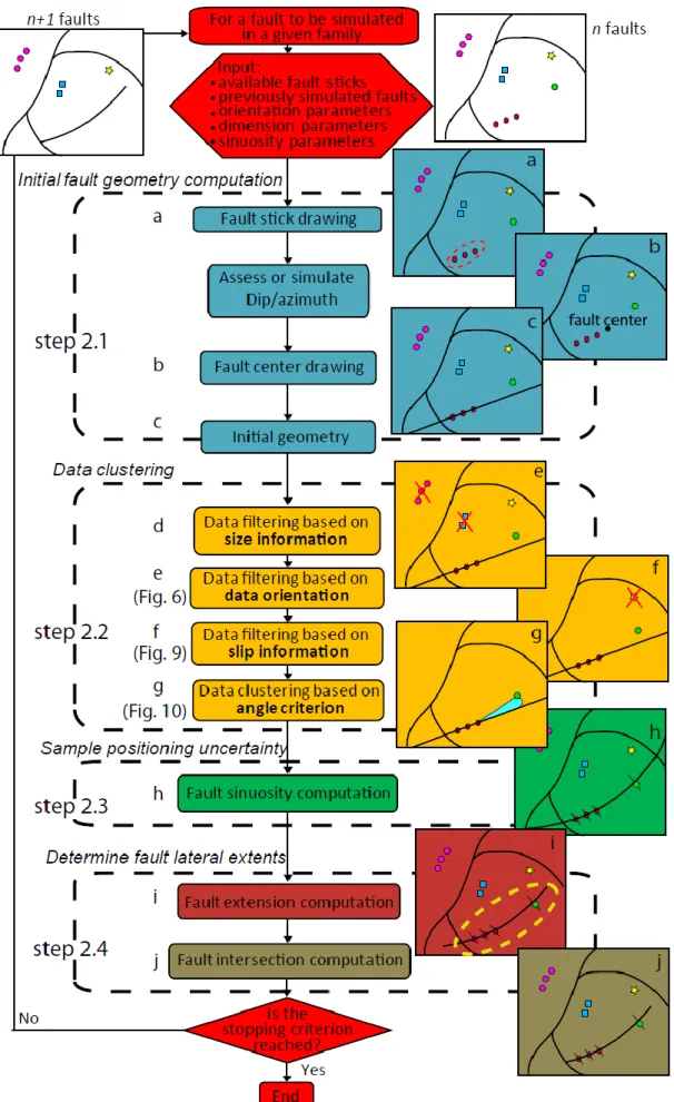
an older fault. More complex configurations such as splay faults and faults being displaced by younger faults are currently not handled in our simulation method. From the input data, the overall stochastic structural modelling strategy first simulates fault surfaces to gener-ate a fault array, then genergener-ates possible stratigraphic models. This process is summarized in Figure 1 and further described below:
1. Prepare the data:
1.1. Interpret fault data to create fault sticks (e.g., by picking likely faults traces on seismic sections).
1.2. Attach information about displacement and location uncertainty to these fault sticks.
1.3. Associate fault sticks to fault families based on orientation and, when relevant, displacement information. By default, a fault stick may correspond to a fault of any family.
1.4. Interpret horizon data to create horizon lines and points.
2. Start the iterative fault simulation: For each fault family by decreasing age,
Do: Simulate a current a fault F
2.1. If fault sticks not yet associated to the fault exist in the current family, randomly select a fault stick and generate an initial geome-try for fault F, honouring the data points S and the fault orientation and center. 2.2. Try to cluster some fault sticks with S, so
that F honours several fault sticks. 2.3. Perturb the initial fault geometry
account-ing for data and interpolation uncertainty. 2.4. Work out the lateral and vertical
termina-tions of fault F and its branching onto oth-er faults.
While: Fault sticks remain to be processed and target number of faults is not reached.
3. Build the stratigraphy:
3.1. Generate a reference 3D stratigraphy honour-ing horizon data.
3.2. Perturb the 3D stratigraphy to reflect data and interpolation-related uncertainties.
Input data and ancillary information
Location information
The fault and horizon traces picked on seismic sections, interpretive paper cross-sections or maps make up the
Fig. 1. Flow chart showing the
general simulation process.
primary input of our method. Point data may also be taken as input, but we will mainly discuss lines in the following because they correspond to the common output of seismic interpretation and provide useful information such as apparent dip. Owing to picking approximations, limited resolution of subsurface data and georeferencing and time-to-depth conversion errors, the exact location of these traces may be uncertain. Therefore, an uncertainty is attached to traces using a radial probability distribution
around line points (Fig. 2), similarly as in Lecour et al. (2001), Wellmann et al. (2010). The more general model of Røe et al. (2014) for point uncertainty could also be used. During fault simulation, each fault trace (also named fault stick) will be associated to a fault surface. To avoid inconsistencies in these surfaces, we now de-scribe additional geometric information which can be associated to each fault trace.
Fig. 2. Example of interpretation data on a vertical seismic
section. Two seismic reflectors have been picked and are shown as green and orange lines. A fault trace is represented as a set of points (white squares); red spheres (in red) around each point represent the uncertainty about these fault picks. The maximum fault throw associated to the fault trace (in black, 60m in this example) is estimated and attached to the fault trace.
Fig. 3. Ambiguity about fault trace information. Many faults
may honour a fault trace interpreted on a 2D section. Example of two fault surfaces representing two different faulting events honouring the same fault trace.
Orientation information from fault traces
As a fault trace is a 2D interpretation on a seismic section or map, the dip of a fault trace does not represent the true dip of the fault. Indeed, the apparent dip on a cross-section is smaller than the true fault dip, unless the seis-mic section is strictly perpendicular to the fault strike:
) sin( ) tan( )
tan(dipapparent diptrue
, (1) where α is the angle between the cross-section and the fault strikeEquation (1) basically tells that the uncertainty about the true dip is small only when the cross-section is almost orthogonal to the fault strike. In practice, the angle α is unknown so little information can be deduced from
ap-parent orientation alone (Fig. 3), but this information may be used to assign a fault to a fault family.
Slip information
Geological maps and cross-sections do not only provide location and orientation information about faults but also indications about the fault slip (Fig. 2). In seismic data interpretation, semi-automatic methods may also esti-mate such information. For instance, Liang et al. (2010) proposed the computation of throw vectors based on cross-correlation of adjacent seismic traces.
In this work, we associate to each fault trace a positive value representing the maximum vertical slip component. This information is used to constrain the fault size and obtain coherent displacement profiles on the simulated faults. The discrimination between fault types (normal or inverse) is made when assigning each fault trace to a given fault family characterized by a type and a strike and dip distributions. A signed slip value could also be relevant in tectonically complex domains where strike-slip is dominant or when fault throw may have been reversed owing to fault reactivations.
Size/Slip model
In the field, faults are never observed entirely. Uncertain-ties about lateral fault extent also exist in the presence of 3D seismic data because faults are not easily identified when the displacement is below seismic resolution. Through several systematic studies, it has been shown that the maximum displacement dmax and fault size L are
generally related by a power law (Yielding et al. 1996; Kim & Sanderson 2005):
𝑑𝑚𝑎𝑥 = 𝑐𝐿𝑛, with 𝑛 ∈ [0.5, 2]. (2)
This information is very interesting in the context of stochastic fault simulation because it provides a con-straint on fault size based on the observed displacement. The exponent n is often assumed to be equal to 1 (Kim & Sanderson 2005). The factor c corresponds to the dis-placement at unit length and may be estimated from analogues.
On a cross-section, the maximum observed vertical dis-placement (fault throw) is only an approximation of the true one owing to several factors:
The maximum throw may not be observed, so the fault size may be under-estimated.
Some faults may be missed or misinterpreted during interpretation, e.g. two close faults may be interpreted as one single fault leading to an over-estimation of the fault size.
Therefore, a possible perspective could be to use random variables to sample parameters c and n in order to ac-count for uncertainty about the maximum observed throw and the approximate nature of this type of statistical model.
Fig. 5. Fault represented as an implicit surface. The fault is
defined by the equipotential f of a volumetric scalar field
DF(x,y,z). Fault families
Characteristic fault shape parameters can be summarized through statistical distributions of size, orientation and sinuosity. Similar faults are grouped into fault families, each family relating to a given faulting event character-ized from regional tectonic knowledge, e.g. a NW-SE extension or a W-E transtension. Fault families are ranked chronologically to represent the time sequence of the fault events and to model observed fault truncations: a fault terminates on or crosses existing faults.
Fault traces are assigned to specific fault families when possible:
If the global fault orientation is believed to be almost perpendicular to seismic sections (e.g. from regional context), fault traces can be re-stricted to some fault families based on apparent orientation, e.g., to distinguish opposed-dipping faults.
If the throw information is sufficient to discrim-inate the fault type for a given fault trace, the fault trace can be restricted to belong to specific fault families corresponding to this particular fault type.
When fault traces are assigned to several fault families, only the simulated faults of these families can honour these fault traces.
Additionally, families contain information about the target number of fault surfaces to be simulated. The actu-al number of faults in a reactu-alization may be equactu-al to that target if it is sufficient to honour all fault sticks, or larger otherwise.
Stratigraphic information
The stratigraphic data corresponds to points or lines representing stratigraphic horizons interpreted on seismic sections, either manually or using horizon tracking tools. As compared to fault data which are associated to fami-lies, horizon points or lines are associated with layering
information in the form of a stratigraphic column. This piece of information is essential to generate layer geome-tries, especially in the presence of unconformities. Addi-tionally, stratigraphic orientation as observed on wells may be used as input, both on main stratigraphic hori-zons and within layers (see Caumon et al. (2013) for details).
Fault network simulation
The method proceeds iteratively by fault family (Fig. 1). We now describe the elementary steps for simulating one fault of a given family, see also Figure 4. For the sake of simplicity, we assume below that each fault to simulate contains at least one fault pick (otherwise, the fault pa-rameters are simply drawn randomly from the statistical information associated to the current fault family).
Step 2.1: Initial fault geometry computation
A fault trace S is first randomly drawn from the input fault data (Fig. 4a). If the average plane of the fault trace is inconsistent with the orientation distribution of the associated fault family, the dip and the strike are random-ly drawn from that distribution. Then, a fault centre is randomly drawn in the neighbourhood of S (Fig. 4b). This fault centre is drawn in a volumetric probability distribution function, which is uniform if no input infor-mation is provided. This distribution may also account for the distance to other faults, e.g. to simulate secondary faults occurring in the vicinity of existing major faults (conditional distribution law), or conversely to emulate screening effects (Ackermann & Schlische 1997). At this point, fault parameters (fault trace S, orientation and centre) are used to define the initial fault geometry (Fig. 4c). In our implementation, a fault is an implicit surface defined as the equipotential f of a volumetric scalar field DF(x,y,z) within a given volumetric domain A
meshed with tetrahedra (Frank et al. 2007; Caumon et al. 2013):
𝐷𝐹(𝑥, 𝑦, 𝑧) = 𝑓, ∀ (𝑥, 𝑦, 𝑧) ∈ 𝐴. (3) Each simulated fault is defined by its own scalar field (Fig. 5). The interpolation is performed in a tetrahedral mesh and scalar field values are stored on the mesh verti-ces. This scalar field is computed by numerical optimiza-tion as described by Frank et al. (2007) and Caumon et
al. (2013), which makes it convenient to rapidly update
the fault geometry in further steps.
Step 2.2: Data clustering
Once an initial fault surface has been computed, availa-ble fault traces are considered as candidates for possiavaila-ble inclusion in the fault surface being built. Therefore, the algorithm first performs a three-step filtering in order to ensure plausible fault geometry and slip profile. All available fault traces from the same family are consid-ered as candidates by the set of filtering rules below.
Data filtering based on size information (Fig. 4, d)
Depending on the target fault size as defined in the cur-rent fault family, fault traces that are too far away from the current fault centre are discarded. Indeed, their inclu-sion in the fault would lead to a fault too long as com-pared to the input size distribution for the family. Addi-tionally, fault sticks which are not in the same fault block as the fault centre may be ignored to avoid crossing con-tacts between faults. With our current representation of fault blocks based on extrapolated faults, this option is generally irrelevant because it tends to generate smaller and smaller faults as simulation proceeds
Data filtering based on data orientation(Fig. 4, e)
In general, fault traces with opposed dip should not be clustered, because it would imply significant changes in fault dip and unrealistic stratigraphic geometry. For a given fault trace S, we propose to compute the distance between the furthest point 𝑝𝑓 and the closest point 𝑝𝑐 projected onto the fault surface, respectively 𝑝𝑓𝑖𝑚𝑝𝑎𝑐𝑡 and 𝑝𝑐
𝑖𝑚𝑝𝑎𝑐𝑡. The angle 𝛼′ between the vectors 𝑣
𝑆(𝑝𝑓, 𝑝𝑐) and 𝑣𝑆𝑖𝑚𝑝𝑎𝑐𝑡(𝑝𝑓𝑖𝑚𝑝𝑎𝑐𝑡, 𝑝𝑐
𝑖𝑚𝑝𝑎𝑐𝑡
) is then computed. Clustering is not allowed if 𝛼′ is deemed too large, which ensures an acceptable dip change in case of clustering (Fig. 6). In case S is sub-horizontal, this strategy avoids clustering data points that would entail a too large strike change for the fault being built. In practice, 𝛼′ should not be chosen greater than 30o to ensure realistic orientation changes.
This strategy could be modified to allow for listric fault geometries.
Data filtering based on throw information (Fig. 4, f)
The maximum throw attached to fault traces provides useful information that can help clustering fault traces in a consistent way. Indeed, the slip amplitude is often assumed to be sub-maximum to maximum at the fault centre and null at fault tip-line (Barnett et al. 1987; Walsh et al. 2003) (Fig. 7).
Therefore, a fault honouring a trace S with maximum displacement dS may or may not be clustered with a trace
S’ with maximum displacement dS’ depending on the
following configurations:
(1) If S and S’ are on both sides of the fault centre, no rule applies, so clustering is possible (trace
S0’ in Figure 8);
(2) If S’ is between S and the fault tip-line, dS’
should be smaller than dS (trace S2’ in Figure 8);
(3) If S’ is between S and the fault centre, dS’ should
be larger than dS (trace S1’ in Figure 8).
These rules must be strictly applied in the case of isolat-ed faults but are not appropriate when faults are close and interact because the displacement profile may then be more complex. They do not apply either if faults have grown by segment linkage (Walsh et al. 2003). Conse-quently, a tolerance ε is introduced for more general fault displacement profiles, which yields the following updat-ed rules in cases 2 and 3:
Fig. 6. Fault trace filtering based on orientation. The closest
and furthest points of each trace S1 and S2 from fault F are
projected onto F. Angle 𝛼1′ is too large so F cannot honour S1
whereas 𝛼2′ is small which enables F to possibly honour S2. The
filtering ensures reasonable dip or strike changes in case the fault trace is sub horizontal.
Fig. 7. Isolated fault displacement distribution. The fault
dis-placement is maximum at the centre of the fault and null at tip-line.
Fig. 8. Fault trace filtering based on displacement infor-mation. The fault honours the fault trace S with attached displacement dS and three other fault traces 𝑆0′, 𝑆1′, 𝑆2′ (with respectively displacement 𝑑𝑆1′, 𝑑𝑆2′ and 𝑑𝑆3′) are candidates for clustering. Fault trace 𝑆0′ is not on the same side of the fault centre than S; therefore 𝑆0′ is not filtered out because no rule applies. Fault trace 𝑆1′ is between S and the fault centre, so 𝑑𝑆1′ should be larger than dS (Eq. (3)) for considering 𝑆1′ as candidate for clustering. Fault trace 𝑆2′ is between S and the fault tip-line, so 𝑑𝑆2′ should be smaller than dS (Eq. (2)) to consi-der 𝑆2′ as candidate for clustering.
If S’ is between S and the fault tip-line, dS’ must
sat-isfy:
𝑑𝑆′ ≤ 𝑑𝑆(1 + 𝜀). (4) If S’ is between S and the fault centre, dS’ must
sat-isfy:
𝑑𝑆′ ≥ 𝑑𝑆(1 − 𝜀). (5) If these relations are not honoured, S’ is not associated with S. Other rules could also be considered to constrain data clustering. Indeed, if the difference of displacement observed at two relatively close fault sticks is large, these two fault sticks are unlikely to belong to the same fault because it would imply the stratigraphy to be highly curved along the fault strike. This may also be the sign of a branching fault occurring between the fault sticks.
Data clustering based on angle criterion (Fig. 4, g)
The three previous processing steps aim at filtering kin-ematically inconsistent fault sticks. Then, remaining fault sticks are considered as candidates for possible clustering with the fault being built. The data clustering probability of each candidate relies on the angle α it forms with the initial fault surface (Fig. 9) (Cherpeau et al. 2010a). Small α angles entail small fault surface changes as
com-pared to large α angles, hence are considered more likely,
i.e. the smaller α, the higher the probability of clustering.
The algorithm first defines a Gaussian cumulative distri-bution function CDFc(α): the distridistri-bution is centred (mean 0) and its standard deviation is arbitrarily chosen to 20 degrees. For a fault stick with angle α, the algo-rithm computes the probability of clustering pc(α) as follows (Fig. 10):
𝑝𝑐(α) = 1 − |0.5 − 𝐶𝐷𝐹𝑐(α)| × 2
Therefore, a fault stick with α equal to zero is systemati-cally considered for clustering and the probability of clustering is equal to 0.32 for α=20˚, which limits high curvature changes. The mean m of CDFc(α) is updated to be the mean of α angles of accepted fault sticks in order to only draw coherent fault sticks. From a computational point of view, this methodology avoids updating the fault geometry and α angles each time a fault stick is drawn.
Steps 2.3 and 2.4: final fault geometry computation
Fault sinuosity (Fig. 4,h)
Once data clustering has been performed, the fault scalar field is updated so that the fault equipotential surface passes through the retained fault traces. This is achieved by using all traces in the optimization of the scalar field
DF (Eq. (3)). Then, the fault scalar field is stochastically
perturbed to obtain the final fault geometry. The pertur-bation consists in adding a correlated random field gen-erated by a conditional Sequential Gaussian Simulation whose parameters are determined from the input sinuosi-ty parameters. The value of the random field is set to zero at conditional fault trace locations if no uncertainty exists. If a perturbation range is attached to fault traces, the value of the perturbation is drawn from a triangular law whose mode is the current location. As in Lecour et
al. (2001), a probability field simulation (Srivastava
1992) is used to provide the random numbers in order to ensure a correlated geometry between data points.
Fault extension (Fig. 4,i)
The next simulation step consists in modelling the exten-sion of the fault. For that, we represent the fault existence domain A (Eq. (2)) by thresholding a 3D scalar field (Cherpeau et al. 2011). This scalar field is initialized analytically with a 3D ellipsoid around the fault centre. Without any further information and based on previous studies (Barnett et al. 1987; Walsh et al. 2003), the 3D ellipsoid is built from size parameters simulated from the input statistical distributions given by the users. It is also possible to use displacement/size statistical relationships to randomly draw the fault size, see Eq. (2).
Fault intersection (Fig. 4,j)
The simulated fault may intersect previously simulated faults, hence the final step consists in honouring fault intersections. The algorithm first tests the intersection with neighbour faults using a Binary Partition Tree that describes the fault spatial layout (Fuchs et al. 1980).
Fig. 9. Data clustering based on angle criterion (map view). (a)
The angles αi between data points and the initial fault surface
are computed (map view). The probability of clustering in-creases when αi decreases. (b) Example of different fault
sur-faces corresponding to different data clustering. From Cherpeau
et al. (2010a).
Fig. 10. Probability law of data clustering. The probability pc(α) depends on the angle α between data points and the initial
fault surface (Fig. 9). If α equals zero, it means the data points are already on the fault surface, thus the clustering probability is 1. The probability pc(α) is symmetrical about the zero angle and quickly decreases towards large angles to avoid sinuous faults.
Fig. 11. Partial branching between two faults. In the case of
partial branching, the algorithm may consider it as a crossing contact (in which the two faults are conjugate, a) or branching contact (in which the fault assumed youngest is truncated by the other fault, b).
Then, it propagates to further faults only if needed so as to limit computational time.
In some cases, the outline of the simulated fault inter-sects another fault in only one point (partial branching, see Figure 11). To our knowledge, this type of configura-tion has received little attenconfigura-tion in the literature, either because it is never observed on outcrop or simply be-cause it does not exist in nature. In such a case, we pro-pose the fault contact to be considered either as crossing (Fig. 11a) or branching (Fig. 11b).
Stopping criterion
A target number of faults is given as input for each fault family. It can be estimated by the supposed number of fault traces per fault, regional analogues, other prior information or modelling constraint. The simulation process continues as long as the number of simulated faults is smaller than the input number of faults or some fault traces are still available, i.e. fault traces not includ-ed in any simulatinclud-ed fault. The number of faults may also be randomized so that the algorithm generates fault net-work realizations with varying numbers of faults (Cherpeau et al. 2012).
Stratigraphic modelling
Computing the stratigraphy
The method uses implicit surfaces to represent fault sur-faces. Consequently, the tetrahedral mesh supporting the fault simulation is not conformable to the simulated faults. However, these discontinuities need to be intro-duced into the mesh to be able to compute the strati-graphic field with displacement along fault surfaces (Caumon et al. 2013). This work uses a resampling and point insertion Delaunay method implemented in the SKUA software to compute fault blocks from fault sur-faces (Lepage 2003; Jayr et al. 2008). Then, one or sev-eral stratigraphic fields DS(x,y,z), depending on the
num-ber of stratigraphic unconformities, are interpolated through the faulted model with horizon data guiding and constraining the process in a deterministic manner (for more details, see Frank et al. (2007); Jayr et al. (2008) and Caumon et al. (2013)).
Stratigraphy-related uncertainty
Stratigraphic horizon uncertainties can be divided into two terms:
A continuous uncertainty about the horizon depth away from the boreholes and cross-sections. In sparse data settings, it mainly consists of interpola-tion and interpretainterpola-tion uncertainties. In seismic da-ta settings, it relates to time-to-depth conversion and hence to the uncertainty about the velocity field in the overburden (Abrahamsen 1992; Thore
et al. 2002). This term can be sampled by
perturb-ing horizon geometry while preservperturb-ing the fault displacement fields. It generally represents the first order uncertainty.
A discontinuous uncertainty reflecting the uncer-tainty about the fault displacement field (Suzuki et
al. 2008). This uncertainty can be significant away
from cross-sections in 2D data settings. In the pres-ence of 3D seismic data, this uncertainty may also be large in poorly imaged areas such as in subsalt structures.
These two uncertainties are handled by adding two corre-lated random fields (Fig. 12, middle) to the initial strati-graphic scalar field (Fig. 12, top) to obtain the final ge-ometry (Fig. 12, bottom) (Caumon et al. 2007, Caumon 2010). This correlated noise is computed in the deposi-tional space (Mallet, 2014) for the continuous term (R1(x,y,z)) (Fig. 12, middle left), which ensures a
coher-ent layer perturbation across faults. A second random field R2(x,y,z) is computed in the xyz Cartesian space to
model the discontinuous term (Fig. 12, middle right) with locally varying anisotropy aligned on the stratigraphic orientation. This second random field is discontinuous across faults to account for fault throw uncertainty. As such it is computed directly on the tetrahedral mesh through an extension of the GsTL algorithms (Remy et
al. 2002) to the tetrahedral SKUA data structure. In both
cases, the random field is set to zero at data location to guarantee data conditioning.
Specific care is needed to ensure a homogeneous pertur-bation of the stratigraphic scalar field DS(x,y,z). Indeed,
the random noise has to be scaled by the local norm of the gradient of DS(x,y,z) so that the amplitude of
pertur-bation in meters can be considered even if the layer thickness varies over the domain of interest (Caumon 2010). The perturbed stratigraphic field 𝐷𝑆′(𝑥, 𝑦, 𝑧) is obtained as follows (figure 12, bottom):
𝐷𝑆′(𝑥, 𝑦, 𝑧) = 𝐷𝑆(𝑥, 𝑦, 𝑧) + 𝑅1(𝑥, 𝑦, 𝑧) × |∇𝐷𝑆(𝑥, 𝑦, 𝑧)| + 𝑅2(𝑥, 𝑦, 𝑧) × |∇𝐷𝑆(𝑥, 𝑦, 𝑧)| (6) Consequently, several stochastic stratigraphic fields can be generated for a given fault network realization. Mallet & Tertois (2010) similarly account for geometric uncer-tainty about faults and horizons but their methodology relies on a preferred deterministic geometric model (Mal-let, 2014). Here, this uncertainty compounds with that which is sampled by the stochastic fault network realiza-tions.
Simulation choices: discussion
The simulation process presented above generates sto-chastic structural models to account for possibly large structural uncertainties. The various parameters describ-ing a fault surface (choice of fault traces, orientation, centre, sinuosity, and dimension) are simulated sequen-tially for each fault. The relative order of these steps is arbitrary and could be changed; for instance, the fault extension could be simulated before the data clustering step. In this case, the clustering rules would be stricter as the method actually takes the maximum fault size from input distribution. The fault centre could also be drawn after the data clustering to allow for more fault trace inclusion possibilities. However, we consider the fault centre as being a crucial parameter because it determines the neighbourhood of the future fault. This choice is also motivated by the perspective of including more input information during the fault nucleation step, e.g. to fa-vour nucleation in high displacement areas and avoid nucleation in low displacement areas.
In general, the simulation steps should first randomly draw the fault characteristics which are most constrained by observations. Then, these well constrained fault pa-rameters should help constraining the simulation of the less informed fault characteristics, along with geological rules, physical laws or prior geological knowledge. In some geodynamic contexts, recent faults may also displace older ones; this is not presently allowed in the current workflow. This may be emulated by simulated older faults as independent surfaces on the more recent fault surface. Several strategies need to be considered to add such poly-phased tectonics in the proposed algo-rithm; some recent related works such as vector-field based deformations open interesting avenues to address this problem (Bouziat 2012; Laurent et al. 2013).
Fig. 12. Method for modelling stratigraphic uncertainty. Top: initial geometry. Middle: the uncertainty is composed of a stratigraphic
and a Cartesian correlated random fields. Bottom: updated horizon geometry which corresponds to the sum of the initial geometry with the perturbations fields.
Application to a Middle East field case
In this section, we propose to illustrate the methodology on a Middle East field to show the impact of both fault and horizon uncertainties on gross rock volume (GRV) estimations in a sparse data situation such as encountered from exploration to development phases. One of our main objectives here is to consider how much fault un-certainty affects the GRV as compared to considering deterministic fault network and solely assessing reservoir depth and thickness uncertainty. The studied area is ahorst with normal faults and three main horizons overly-ing three stratigraphic reservoir units.
Input data
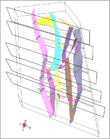
Both horizons and faults are interpreted on five fictive seismic lines orthogonal to the regional horst direction. These five lines and the associated 2D structural interpre-tations are generated from a 3D seismic dataset and the corresponding reference interpretation (Fig. 13). For each fault trace S, the maximum vertical offset of horizons on
Fig. 13. The reference interpretation has been built from a full
3D seismic survey. Faults and horizons have been interpreted on five fictive seismic lines. Fault traces have been grouped according to their orientation. SW dipping traces (green colour) are set to belong to family1. NE dipping traces (yellow colour)
are set to belong to family2. Other fault traces (pink colour) are
not classified hence can correspond to a fault from any fault family. Scale is not given and orientation has been modified for confidentiality reasons.
both sides of the fault is measured and associated to S in the data base. Interpreted data are composed of twenty-five fault traces and data points corresponding to strati-graphic horizons. Uncertainty about fault location is set to 10m for each fault trace to reflect picking and migra-tion uncertainty, with a triangular radial probability func-tion centred on the reference locafunc-tion. In this scenario, uncertainty in time-to-depth conversion is assumed neg-ligible as compared to the uncertainty due to the lack of data between the sections, so horizon picks are consid-ered deterministic. For confidentiality reasons, orienta-tion has been changed from original data, GRV unit is arbitrary, the stratigraphic ages and scale are not given.
Fault network characterization
Fault families
From the interpreted fault traces and regional context, faults are grouped into two normal fault families corre-sponding to an east/west extension:
(1) family1 strikes [N80-N100] and dipping [60-70].
Most traces seem oriented along that direction
(green data points in Figure 13) and the mini-mum number of faults in the area is set to 5. (2) family2 corresponds to opposed-dipping faults,
hence is oriented [N260-N280], dips [60-70] (yellow data points in Figure 13) and the mini-mum number of faults in the area is set to 3. For both families, the maximum number of faults is at most equal to the number of fault sticks in that family. In this particular study, we choose to keep the models as simple as possible by stopping the fault simulation as soon as all fault sticks belonging to a given family have been associated to a fault surface. Therefore, the actual number of faults in each realization only depends on the outcome of the fault stick clustering procedure described above.
From regional reservoir analogues, a third fault family,
family3, oriented [N160-N180] with dip uniformly
dis-tributed in [60-70] is also expected. The number of faults for family3 is set to 2. The relative age of the two first
fault families cannot be deduced from the available data and tectonic history, so families are considered cogenet-ic, i.e. there is no systematic truncation rule between faults from different fault families. The third fault family,
family3, is considered branching on the two first families,
so the algorithm simulates first family1 and family2. Fault size
The size/slip model (Eq. (2)) introduced previously is used to estimate the fault size. In the absence of regional analogue data, we use the coefficient 𝑐 = 0.02 provided by Kim & Sanderson (2005) for normal faults.
The throws observed on the seismic sections range from 20 to 260m, which corresponds to a maximum fault elongation of 13km. As discussed above, this can be considered as a lower bound of the actual throw because largest throw amplitude may occur between sections.
Stratigraphic uncertainty
The layer geometry is perturbed by adding random field realizations to the implicit stratigraphic model in SKUA. These perturbation fields are simulated using a Sequen-tial Gaussian Simulation conditioned to be zero at hori-zon picks. The perturbation amplitude is considered centred Gaussian in both cases, with zero mean and standard deviations 𝜎1= 17m for the continuous uncer-tainty and 𝜎2= 8m for the discontinuous uncertainty. Gaussian variograms are used for both continuous and discontinuous stratigraphic uncertainties in order to ob-tain smooth perturbations. Variogram ranges are equal to 2,500m horizontally and 600m vertically for the continu-ous term R1. The discontinuous term R2 is modelled with
a variogram having ranges equal to 1,000m horizontally and 300m vertically.
Results
Fault networks
190 fault networks have been simulated using interpreted fault traces and input fault families. All realizations have
Fig. 14. Gross rock volumes (GRV) distributions for units U1, U2, U3 and total volume (unit is arbitrary for confidentiality reasons)
for case A (topological uncertainties about both faults and stratigraphy, in blue) and case B (uncertainty in the stratigraphy only, in yellow). P10, P90 and interquartile range (IQR) are represented for both cases. The reference model (red arrows) corresponds to a medium case for all units, but case A entails much larger GRV uncertainty than case B.
a larger number of faults than the reference one (Fig. 13) because most simulated faults contain less fault traces than the reference model. This may be explained by:
Clustering rules (displacement profile, orientation deviation) that are too restrictive.
Fault size underestimation, due to an approximated maximum slip or inappropriate parameters c and n in Equation (2). Indeed, if we consider the largest fault in the reference model and assume n equal to one, the parameter c is equal to 0.013 whereas we used 0.02 in the simulation. This may suggest that some faults have been merged in the reference in-terpretation or that some have grown by segment linkage.
In a real situation, no reference model would be available so we chose to proceed with the stratigraphic and gross rock volume uncertainty assessment using all the 190 stochastic fault networks.
Gross Rock Volumes (GRV)
For each stochastic fault network, five stratigraphic fields have been computed by adding the stratigraphic field
obtained by interpolating horizon data through the fault blocks with a random noise composed of the first and second order perturbation R1 and R2. Consequently, 950
structural models have been generated using the method presented above. These models, referred to as case A, were then used to study the uncertainty on the gross rock volumes above a deterministic planar water-oil contact with no transition zone located at 2800m depth in the three distinct stratigraphic units.
To compare the GRV uncertainty accounting for topolog-ical fault uncertainty method with classtopolog-ical uncertainty models which consider fixed fault networks, we also generated a case B comprised of 950 models obtained by perturbing only the stratigraphy of the reference fault model. The chosen stratigraphic uncertainty parameters were the same as in case A. Results for cases A and B are presented in Figure 14.
The GRV values for case B are close to the GRV values of the reference model, the difference between the mean GRV estimation being only 0.02%. In case A, the total GRV mean is about 1% greater than in the reference
Fig. 15. Example of stochastic models (top reservoir surfaces). Top horizon is painted by the depth and contour lines for: (a.) the
reference model, (b.) a pessimistic scenario, (c.) a medium scenario and (d.) an optimistic scenario. The black lines represent cross-sections of Figure 16. Black points correspond to horizon data of the top reservoir. Red points correspond to the locations of the reference faults at the top reservoir (fault data are not visible because they are below the top reservoir). The difference in GRV esti-mation may be explained by a deeper top reservoir in the southern part of the studied area for the pessimistic scenario and a higher top reservoir in the eastern part for the optimistic scenario. These zones contain few data, leading to a relatively large variability in the simulated models.
estimation but 4% greater for unit U1 (volumes in units
U2 and U3 are correlatively lower). For all three units,
the GRV interquartile range is about five times larger in case A than in case B. This highlights the large impact of uncertainty about fault definition and connectivity on the output volumetric uncertainty.
Top reservoir surfaces of a pessimistic scenario (small gross rock volume), a medium scenario (volume similar to the reference) and an optimistic scenario (volume larger than the reference) are presented in Figure 15 and cross-sections of these scenarios are shown in Figure 16. Thanks to the prior definition of fault families and the fault trace clustering rules, the generated fault networks
and the associated displacements seem globally con-sistent and plausible in three dimensions.
These results show that considering fault geometry and connectivity uncertainty may be crucial for assessing accumulation uncertainty when only sparse data are available. Indeed, whereas the reference model corre-sponds to a medium scenario both with and without fault uncertainty, the low case (P10) and high-case (P90) cov-er a much largcov-er range when unccov-ertainties about faults are accounted for. This confirms that considering signifi-cantly varying interpretations and scenarios in poorly constrained reservoir studies is necessary to appropriate-ly address uncertainties and to support field appraisal and development decisions.
Fig. 16. Example of stochastic models (cross-sections). Cross-sections AB (location shown in Figure 15) correspond to: (a.) the
reference model, (b.) a pessimistic scenario, (c.) a medium scenario and (d.) an optimistic scenario. Some faults may be interpreted on all cross-sections owing to the proximity of fault traces (e.g., faults F1 and F3 from family1 and fault F2 from family2). The slip of
fault F1 is larger for the pessimistic scenario so that the hanging wall is below the water-oil contact. The optimistic scenario seems to
contain more faults of family2 than other scenarios, which entails the uplift of tilted foot walls.
Conclusions
The presented work sets the basis for a full stochastic structural modelling workflow. The method starts by the characterization of faults using hard data, geological concepts and physical laws to help determining fault parameters that cannot be directly measured. Then, the stochastic fault model samples both geometrical and topological fault uncertainties. During the next step, one or several stratigraphic fields, depending on the number of unconformities, are computed and stratigraphic uncer-tainties are considered by adding a correlated random perturbation in both depositional and present-day spaces. Consequently, the method generates structural models with various fault connections, number of faults, fault slips and stratigraphic units without limiting assumptions about fault and horizon geometry. This set of models can then be used for making predictions such as gross rock volumes as presented on a Middle East field case study,
which enables to better evaluate risks and be more confi-dent for decision-making in exploration and development settings. Such a stochastic approach is most relevant in sparse data situations, because of the large uncertainties and broad range of possible models that cannot be sam-pled by geometrical perturbations of a single determinis-tic model.
In the presented workflow, the algorithm first generates fault surfaces, using fault displacement information at the data clustering step. Then, the fault displacement is com-puted using horizon data. Whereas faults can be seeded so as to reproduce interactions, some of the generated fault networks are not fully consistent. In particular, no check is made during fault simulation to ensure that the simulated faults have a globally consistent displacement field compatible with horizon data. One solution could consist in adding an extra step at the end of a fault object simulation to directly simulate a fault displacement field according to the fault size. Then, the algorithm could
compare the global measured displacement to the current simulated displacement field and use this information to: (1) nucleate new faults where observed displacement is still greater than the simulated one; (2) avoid nucleation where no displacement has been observed and (3) stop the fault simulation when all displacement is honoured given a tolerance threshold. Instead of interpolating a stratigraphic field constrained to horizon data, the dis-placement of geological layers could also be modelled accounting for the rock behaviours, e.g. to model drag folds, directly in the vicinity of faults (Røe et al. 2010, Laurent et al. 2013).
These improvements would constrain the simulation process to obtain more realistic results, in particular for the location and slip profile of faults. The geomechanical restoration of the simulated models could also be used to falsify inconsistent models, as done by section balancing. In this study, we have focused on structural uncertainties in sparse data contexts and we only assessed the impact of these uncertainties in terms of hydrocarbon accumula-tions. In exploration studies, the proposed workflow could be connected with seal integrity studies. In ap-praisal and development studies, this method also has potential to be integrated in the rest of the modelling workflow to assess the impact of structural uncertainties on reservoir production. This would be relevant also in the presence of 3D seismic data, where fault connectivity may also be uncertain at the fault segment scale (Julio et
al. 2014). In all cases, structural uncertainty should be
considered jointly with other uncertain parameters such as well correlations (Lallier et al. 2012), fault conductivi-ty, petrophysics and fluid properties.
In practice, the computational time required for such an approach does not allow to consider all possible models but only a subset of models. These models should be carefully selected and ranked, for instance using reser-voir simulation proxies. An avenue for further research is to increase the level of input information directly in the simulation model, for instance by formulating mass bal-ance computations as stochastic simulation constraints. Another avenue is to falsify or update some of the mod-els by computing their likelihood and solving an inverse problem. This can be done by introducing some structur-al concepts not accounted for during the simulation pro-cess, as done by Wellman et al. (2014). Confronting the stochastic models to other types of data (e.g., reservoir production curves) is also interesting to reduce uncertain-ties. For example, Cherpeau et al. (2012) propose a pa-rameterization of faults integrated in a stochastic inverse method and use dynamic information to infer fault char-acteristics and reduce fault-related uncertainties. A future challenge is therefore to include this full stochastic struc-tural method in such inverse problem to consider geolog-ical features all together and not only faults separately.
Acknowledgements
The authors would like to acknowledge the RING-GOCAD Consortium managed by ASGA
(http://ring.georessources.univ-lorraine.fr) for funding this research, as well as Paradigm for providing the SKUA-Gocad software and API. We also acknowledge the petroleum company which provided us with the Mid-dle East field dataset. We also appreciate the construc-tive comments made by two anonymous reviewers which helped us improve this paper.
References
Abrahamsen, P. 1992. Bayesian kriging for seismic depth conversion of a multi-layer reservoir. In:
Soares, A., ed., Geostatistics Troia '92. Volume 1. Fourth International Geostatistical Congress. Qualitative Geolo-gy and Geostatistics 5, Kluwer Academic Publ., 385-398. Ackermann, R. V. & Schlische, R. W. 1997. Anticluster-ing of small normal faults around larger faults. Geology, 25, 1127-1130.
Aydin, O. & Caers, J. K. 2014. Exploring Structural Uncertainty Using a Flow Proxy in the Depositional Domain. In: SPE Annual Technical Conference and
Exhibition, Amsterdam, NL, Society of Petroleum
Engi-neers, http://dx.doi.org/10.2118/170884-MS.
Barnett, J. A. M., Mortimer, J., Rippon, J. H., Walsh, J. J. & Watterson, J., 1987. Displacement geometry in the volume containing a single normal fault. AAPG Bulletin, 71, 925-937.
Bond, C., Gibbs, A., Shipton, Z. & Jones, S. 2007. What do you think this is? "conceptual uncertainty" in geosci-ence interpretation. GSA Today, 17, 4-10.
Bouziat, A. 2012. Vector field based fault modelling and stratigraphic horizons deformation. In: SPE Annual
Technical Conference and Exhibition, San Antonio, TX, USA, Society of Petroleum Engineers,
http://dx.doi.org/10.2118/160905-STU. .
Caumon, G. 2010. Towards stochastic time-varying geological modeling. Mathematical Geosciences, 42, 555-569.
Caumon, G., Tertois, A.-L. & Zhang, L. 2007. Elements for stochastic structural perturbation of stratigraphic models. In: Proc. Petroleum Geostatistics, EAGE,
http://dx.doi.org/10.3997/2214-4609.201403041.
Caumon, G., Gray, G. G., Antoine, C. & Titeux, M.-O. 2013. 3D implicit stratigraphic model building from remote sensing data on tetrahedral meshes: theory and application to a regional model of La Popa Basin, NE Mexico. IEEE Transactions on Geoscience and Remote
Sensing, 51, 1613-1621.
Cherpeau, N., Caumon, G. & Lévy, B. 2010a. Stochastic simulation of fault networks from 2D seismic lines. In:
SEG Technical Program Expanded Abstracts, 29,
2366-2370.
Cherpeau, N., Caumon, G. & Lévy, B. 2010b. Stochastic simulations of fault networks in 3D structural modeling.
Cherpeau, N., Caumon, G., Caers, J., & Levy, B. 2011. Assessing the impact of fault connectivity uncertainty in reservoir studies using explicit discretization. In: SPE
Reservoir Characterisation and Simulation Conference and Exhibition, EAGE,
http://dx.doi.org/10.2118/148085-MS.
Cherpeau, N., Caumon, G., Caers, J. & Lévy, B. 2012, Method for stochastic inverse modeling of fault geometry and connectivity using flow data. Mathematical
Geosci-ences, 44, 147-168.
Frank, T., Tertois, A.-L. & Mallet, J.-L. 2007. 3D-reconstruction of complex geological interfaces from irregularly distributed and noisy point data. Computers &
Geosciences, 33, 932-943.
Fuchs, H., Kedem, Z. M., & Naylor, B. F. 1980. On visible surface generation by a priori tree structures. In:
ACM Siggraph Computer Graphics 14, 124-133.
Georgsen, F., Røe, P., Syversveen, A. R., & Lia, O. 2012. Fault displacement modelling using 3D vector fields. Computational Geosciences, 16, 247-259.
Guillen, A., Calcagno, P., Courrioux, G., Joly, A. & Ledru, P. 2008. Geological modelling from field data and geological knowledge: Part II. Modelling validation using gravity and magnetic data inversion. Physics of the
Earth and Planetary Interiors, 171, 158-169.
Holden, L., Mostad, P., Nielsen, B. F., Gjerde, J., Town-send, C. & Ottesen, S. 2003. Stochastic structural model-ing. Mathematical Geology, 35, 899-914.
Hollund, K., Mostad, P., Fredrik Nielsen, B., Holden, L., Gjerde, J., Contursi, M.J., McCann, A.J., Townsend, C. & Sverdrup, E. 2002. Havana—a fault modeling tool. In:
Norwegian Petroleum Society Special Publications, 11,
157-171.
Irving, A. D., Kuznetsov, D., Robert, E., Manzocchi, T., & Childs, C. 2014. Optimization of Uncertain Structural Parameters With Production and Observation Well Data.
SPE Reservoir Evaluation & Engineering, 17, 547-558.
Jayr, S., Gringarten, E., Tertois, A.-L., Mallet, J.-L. & Dulac, J.-C. 2008. The need for a correct geological modelling support: the advent of the UVT-transform.
First Break, 26, 73-79.
Jessell, M. W., Ailleres, L. & de Kemp, E. A. 2010. Towards an integrated inversion of geoscientific data: What price of geology? Tectonophysics, 490, 294-306. Julio, C., Caumon, G., & Ford, M. 2014. Sampling the uncertainty associated with segmented normal fault in-terpretation using a stochastic downscaling method.
Tectonophysics, 639, 56-67.
Kim, Y.-S. & Sanderson, D. J. 2005. The relationship between displacement and length of faults: a review.
Earth-Science Reviews, 68, 317-334.
Lallier, F., Caumon, G., Borgomano, J. Viseur, S., Four-nier, F., Antoine, C. & Gentilhomme, T. 2012. Relevance
of the stochastic stratigraphic well correlation approach
for the study of
complex carbonate settings: Application to the
Malam-paya buildup (Offshore Palawan,
Philippines). In: Geological Society, London, Special
Publication, 370, 265-275.
Laurent, G., Caumon, G., Bouziat, A., Jessell, M. 2013. A parametric method to model 3D displacements around faults with volumetric vector fields. Tectonophysics, 590, 83-93.
Lecour, M., Cognot, R., Duvinage, I., Thore, P. & Dulac, J.-C. 2001. Modeling of stochastic faults and fault net-works in a structural uncertainty study. Petroleum
Geo-science, 7, S31-S42.
Lepage, F. 2003. Three-Dimensional Mesh Generation
for the Simulation of Physical Phenomena in Geoscienc-es. Ph.D. thesis, INPL, Nancy, France.
Liang, L., Hale, D. & Maučec, M. 2010. Estimating fault displacements in seismic images. SEG Technical
Pro-gram Expanded Abstracts, 29, 1357-1361.
Lindsay, M., Perrouty, S., Jessell, M., & Ailleres, L. 2014. Inversion and Geodiversity: Searching Model Space for the Answers. Mathematical Geosciences, 46, 971-1010.
Mallet, J.-L. 2014. Elements of Mathematical
Sedimen-tary Geology: the Geochron Model. EAGE Publications
B.V.
Mallet, J.-L. & Tertois, A.-L. 2010. Solid earth modeling and geometric uncertainties. In: SPE Annual Technical
Conference and Exhibition, Florence, Italy.
http://dx.doi.org/10.2118/134978-MS.
Remy, N., Shtuka, A., Lévy, B. & Caers J. 2002. GsTL: the geostatistical template library in C++. Computers &
Geosciences 28, 971-979
.
Rivenæs, J. C., Otterlei, C., Zachariassen, E., Dart, C., & Sjøholm, J. 2005. A 3D stochastic model integrating depth, fault and property uncertainty for planning robust wells, Njord Field, offshore Norway. Petroleum
Geosci-ence, 11, 57-65.
Røe, P., Georgsen, F., & Abrahamsen, P. 2014. An Un-certainty Model for Fault Shape and Location.
Mathe-matical Geosciences, 46, 957-969.
Seiler, A., Aanonsen, S., Evensen, G. & Rivens, J. C. 2010. Structural Surface Uncertainty Modeling and Up-dating Using the Ensemble Kalman Filter. SPE Journal, 15, 1062-1076.
Srivastava, R. M. 1992. Reservoir characterization with probability field simulation. In: SPE Annual
Technical Conference and Exhibition, Washington D. C.,
Society of Petroleum Engineers,
http://dx.doi.org/10.2118/24753-MS.
Suzuki, S., Caumon, G. & Caers, J. 2008. Dynamic data integration for structural modeling: model screening
approach using a distance-based model parameterization.
Computational Geosciences, 12, 105-119.
Tarantola, A. 2006. Popper, Bayes and the inverse prob-lem. Nature Physics, 2, 492-494.
Thore, P., Shtuka, A., Lecour, M., Ait-Ettajer, T. & Co-gnot, R. 2002. Structural uncertainties: determination, management and applications. Geophysics, 67, 840-852. Walsh, J. J., Bailey, W. R., Childs, C., Nicol, A. & Bon-son, C. G. 2003. Formation of segmented normal faults: a 3D perspective. Journal of Structural Geology, 25, 1251-1262.
Wellmann, J. F., Horowitz, F. G., Schill, E. & Regenau-er-Lieb, K. 2010. Towards incorporating uncertainty of structural data in 3D geological inversion.
Tectonophys-ics, 490, 141-151.
Wellmann, J. F., Lindsay, M., Poh, J., & Jessell, M. (2014). Validating 3-D Structural Models with Geologi-cal Knowledge for Improved Uncertainty Evaluations.
Energy Procedia, 59, 374-381.
Yielding, G., Needham, T. & Jones, H. 1996. Sampling of fault populations using sub-surface data: a review.