HAL Id: inria-00547254
https://hal.inria.fr/inria-00547254
Submitted on 15 Dec 2010
HAL is a multi-disciplinary open access
archive for the deposit and dissemination of
sci-entific research documents, whether they are
pub-lished or not. The documents may come from
teaching and research institutions in France or
abroad, or from public or private research centers.
L’archive ouverte pluridisciplinaire HAL, est
destinée au dépôt et à la diffusion de documents
scientifiques de niveau recherche, publiés ou non,
émanant des établissements d’enseignement et de
recherche français ou étrangers, des laboratoires
publics ou privés.
Utku Acer, Paolo Giaccone, David Hay, Giovanni Neglia, Saed Tarapiah
To cite this version:
Utku Acer, Paolo Giaccone, David Hay, Giovanni Neglia, Saed Tarapiah. Timely Data Delivery in a
Realistic Bus Network. [Research Report] RR-7344, INRIA. 2010. �inria-00547254�
a p p o r t
d e r e c h e r c h e
N 0 2 4 9 -6 3 9 9 IS R N IN R IA /R R --7 3 4 4 --F R + E N GNetworks and Telecommunications
Timely Data Delivery in a Realistic Bus Network
Utku Günay Acer — Paolo Giaccone — David Hay — Giovanni Neglia — Saed Tarapiah
N° 7344
August 2010
Centre de recherche INRIA Sophia Antipolis – Méditerranée 2004, route des Lucioles, BP 93, 06902 Sophia Antipolis Cedex
Utku Günay Acer
∗†, Paolo Giaccone
‡§, David Hay
¶, Giovanni
Neglia
∗k, Saed Tarapiah
‡∗∗ Theme : Networks and Telecommunications Networks, Systems and Services, Distributed ComputingÉquipe-Projet Maestro
Rapport de recherche n° 7344 — August 2010 — 32 pages
Abstract: WiFi-enabled buses and stops may form the backbone of a metropolitan de-lay tolerant network, that exploits nearby communications, temporary storage at stops, and predictable bus mobility to deliver non-real time information.
This paper studies the problem of how to route data from its source to its destina-tion in order to maximize the delivery probability by a given deadline. We assume to know the bus schedule, but we take into account that randomness, due to road traffic conditions or passengers boarding and alighting, affects bus mobility. In this sense, this paper is one of the first to tackle quasi-deterministic mobility scenarios.
We propose a simple stochastic model for bus arrivals at stops, supported by a study of real-life traces collected in a large urban network with 250 bus lines and about 7500 bus-stops. A succinct graph representation of this model allows us to devise an optimal (under our model) single-copy routing algorithm and then extend it to cases where several copies of the same data are permitted.
Through an extensive simulation study, we compare the optimal routing algorithm with three other approaches: minimizing the expected traversal time over our graph, maximizing the delivery probability over an infinite time-horizon, and a recently-proposed heuristic based on bus frequencies. We show that, in general, our optimal algorithm outperforms the three, but it essentially reduces to either minimizing the expected traversal time when transmissions are always successful, or maximizing the delivery probability over an infinite time-horizon when transmissions fail frequently. For re-liable transmissions and “reasonable” values of deadlines, the multi-copy extension requires only 10 copies to reach almost the performance of costly flooding approaches.
Key-words: Delay Tolerant Networks, Quality of Service, Optimal Routing
∗EPI Maestro, INRIA Sophia Antipolis Mditerrane, France †[email protected]
‡Dipartimento di Elettronica, Politecnico di Torino, Turin, Italy §[email protected]
¶Dept. of Electrical Engineering, Columbia University, NY, USA, [email protected] k[email protected]
Résumé :Bus et arrêts avec capacités de transmission WiFi peuvent constituer l’épine
dorsale d’un réseau urbain tolérant aux délais, qui exploite les transmissions à courte portée, le stockage temporaire des données aux arrêts, et la mobilité prévisible de bus pour délivrer des informations non en temps réel. Cet article étudie le problème de savoir comment router les données à partir de la source jusqu’à la destination afin de maximiser la probabilité de livraison dans un délai donné. Nous supposons que nous connaissons les horaires de bus, mais nous prenons en compte le caractère aléatoire de la mobilité des bus, dû aux conditions de circulation ou au temps nécessaire pour l’embarquement et le débarquement des passagers. En ce sens, le présent document est l’un des premiers à aborder un scénario de mobilité quasi-déterministe. Nous pro-posons un modèle stochastique simple pour les arrivées de bus aux arrêts, motivé par une étude des traces réelles recueillies dans un vaste réseau urbain avec 250 lignes de bus et environ 7500 arrêts de bus. Une représentation graphique succincte de ce modèle nous permet de concevoir un algorithme de routage optimal (conformément à notre modèle) utilisant une seule copie des données, puis de l’étendre au cas où plusieurs copies des mêmes données sont permises. Grâce à une vaste étude de simu-lation, nous comparons l’algorithme de routage optimal avec trois autres approches : minimiser le temps attendu de traversement du graphe, maximiser la probabilité de livraison sur un horizon temporel infini, et un algorithme heuristique récemment proposé basé sur les fréquences de bus. Nous montrons que, en général, notre algo-rithme optimal surpasse les trois autres, mais il se réduit essentiellement à minimiser le temps de traversement quand les transmissions sont toujours couronnées de succès, ou à maximiser la probabilité de livraison sur un horizon temporel infini lorsque les transmissions échouent fréquemment. Pour les transmissions fiables et des valeurs des délais «raisonnables», l’extension multi-copie nécessite seulement 10 copies pour at-teindre quasiment la même performance que celle du flooding, particulierment coûteux en terme de nombre de transmissions et utilisation de buffers.
Mots-clés : French Keywords
1
Introduction
We consider an opportunistic data network formed by (some) buses and bus stops equipped with wireless devices, e.g. based on WiFi technologies, like in DieselNet [13]. Most of the stops act as disconnected relay nodes (the throwboxes in [3]), and a few of them are also connected to the Internet. Data are delivered across town following the store-carry-forward network paradigm [44], based on multi-hop communication in which two nodes may exchange data messages whenever they are within transmission range of each other.
A bus-based network is a convenient solution as wireless backbone for delay toler-ant applications in an urban scenario. In fact, a public transportation system provides access to a large set of users (e.g. the passengers themselves), and is already designed to guarantee a coverage of the urban area, taking into account human mobility pat-terns. Moreover, such a wireless backbone is not significantly constrained by power and/or memory limitations: a throwbox can be easily placed on a bus and connected to its power supply, or be put in an appropriate place in bus stops, which are usually already connected to the power grid to provide lights and electronic displays, but also in any other places where power supply is available. Finally, travel times can be pre-dicted from the transportation system time-table; even if the actual times are affected by varying road traffic conditions and passengers’ boarding and alighting times, such a backbone still provides strong probabilistic guarantees on data delivery time that are not common in opportunistic networks.
Indeed, this paper explores the basic question: “how to route data over a bus-based
network, from a given source to a given destination, so that the delivery probability by a given deadline is maximized?”. We rely on the knowledge of bus schedule information
and some stochastic characterization of bus mobility, obtained from real data traces. We consider two classes of routing schemes over such a network. The first class relies only on forwarding a single copy of the data is propagated along a single path. The second class takes advantage of multiple copies spread in the network to increase delivery probability and reduce delivery time, albeit with higher bandwidth usage.
Another architectural choice is between exploiting only bus contacts, only bus-stop contacts, or both types of contacts. While the latter case should provide better performance, the two kinds of transmission opportunities have very different charac-teristics, making it hard to model both of them together in a common framework. For example, a potential contact between two buses traveling along orthogonal trajectories can be completely avoided if there is even a slight delay of one of them. On the other hand, in case of a bus-stop communication, the contact always happens eventually, but may be delayed. Most prior art (see Sec. 2) considered only bus-bus communications. In this paper, we focus on the other alternative, relying only on bus-stop communica-tions. In Appendix A, we show that bus-stop communications potentially offer better performance in the real bus network scenario under consideration. Further, we present an analysis on connectivity of the bus network using the bus-stop communications in Appendix E.
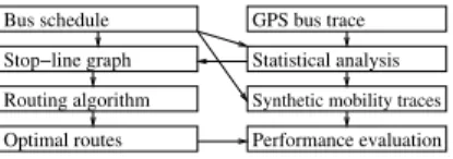
Fig. 1 depicts the high-level framework used in the paper to study routing in the proposed network. Our starting point is a simple mobility model for buses (described in Sec. 3.1), that is supported by the statistical analysis of a set of real traces of the public transportation system of Turin in Italy, which serves an area of about 200 km2through
about 7500 stops and 1500 vehicles distributed among 250 lines. These traces include the complete schedule for a working day and the corresponding GPS traces with the positions of all the vehicles during the morning rush hour period (6 AM–10 AM).
Synthetic mobility traces Bus schedule Stop−line graph Routing algorithm Optimal routes GPS bus trace Statistical analysis Performance evaluation
Figure 1: High-Level Evaluation Framework
A statistical analysis of these traces in Sec. 3.1 yields some important conclusions, that allow us to represent the transportation system appropriately in terms of a graph with independent random weights, that we call the stop-line graph (Sec. 4). Under this representation, our original optimization problem to identify routes maximizing the delivery probability by a given deadline (or maximizing the on-time delivery probabil-ity) becomes equivalent to a specific stochastic shortest path problem on the stop-line graph. We are able to find an optimal algorithm, called ON-TIME, for the single-copy case (Sec. 4.2) and then to extend it for the multi-copy case through a greedy approach (Sec. 4.4). We compare the performance of these proposed algorithms with three other heuristics (Sec. 4.3) that also operate on the stop-line graph: an adaptation of the
rout-ing algorithm proposed in [38] for bus-bus communications (we refer to it as MIN
-HEADWAY), and the two naïve algorithms, MIN-DELAY, that determines the path with the least expected weight, and MAX-PROB, that maximizes the delivery probability on an infinite time-horizon. Since the number of real-life traces we obtained is limited, the comparison (Sec. 5) is based on simulations carried on a large set of synthetic traces generated on the basis of our bus mobility model and the schedule of Turin bus system.
The paper has the following main contributions and conclusions.
1. Formulation of the original routing problem as a specific stochastic shortest prob-lem on a particular stochastic graph, that is justified by a statistical analysis of real transportation system traces.
2. Optimal (under our model) routing scheme for the single copy case. While this offline routing scheme has, in theory, an exponential worst-case time complexity, in practice it is able to find the optimal route in reasonable time, allowing each node to store an optimal pre-selected routing plan.
3. Extensions to multi-copy case, based on greedy approaches applied to the single-copy scheme. We prove a tight bound of 1/k for the on-time delivery probability in comparison to an optimal (non-greedy) k-copy scheme.
4. Simulation analysis showing that the optimal algorithm outperforms the MIN
-HEADWAY heuristic, but it performs as the MIN-DELAY algorithm when the
there is no packet loss, and as MAX-PROBwhen packet losses are significant across the network. We provide some explanation for these results. In this sense the conclusion is that naïve heuristics like MIN-DELAYor MAX-PROB algo-rithms may be very good heuristics for routing over realistic bus transportation networks.
5. Simulations showing that only 10 copies are needed for a multi-copy greedy approach to reach performance close to flooding routing policies; the latter re-quires at least two order of magnitude more transmissions and copies for each single piece of data.
2
Related Work
Employing a bus network as a mobile backbone for dense vehicular networks was first proposed in [47], using standard routing protocols for mobile ad-hoc networks (e.g., DSR or AODV). More recently, buses employment in a disconnected scenario has been considered; e.g. in the seminal DieselNet project [13]. Since our paper considers routing in such a network, in what follows we only mention work related to routing issues.
Most of the research has focused on bus-bus communications [10, 2, 38, 17, 18] with the following routing approach: Each vehicle learns at run time about its meeting process; then, the vehicles exchange their local view with other vehicles and use the information collected to decide how to route data. The goals of the proposed algorithms were either to reduce the expected delivery time or to maximize the delivery probability. Unlike these studies, we mainly focus on bus to stop data transfers and derive a single-copy routing algorithm to maximize the delivery probability by a given deadline. We then extend the algorithm to address settings where several copies of the same data are permitted. On the other hand, we do not consider buffer or bandwidth constraints, (e.g., as in [10, 2]) as they are not a major concern in our settings: When the mobile devices are buses (as opposed, for example, to cellular phones), it is reasonable to assume that there is sufficient storage available; in addition, since buses communicate with stops (as opposed to other moving buses), the amount of data transferable during a meeting is larger. Nevertheless, characterizing the bandwidth of the contacts and incorporating these constraints into our framework for bandwidth-hungry applications is part of our ongoing research.
The use of fixed relay nodes was also considered in [5, 3]. In [5], an architecture is proposed where bus passengers may use the cellular network to require content that will be delivered to access points along the bus trajectory. This data can be replicated also on other buses, taking advantage of possible data transfers between vehicles. Their analysis considers only a simplistic single-street scenario and does not address routing issues. [3] reports that the performance of a vehicular network is improved by adding some infrastructure, like base stations connected to the Internet, a mesh wireless back-bone, or fixed relays (which are similar to our stops). The most important results are (i) there are scenarios where a mesh or relay hybrid network is a better choice over a base station networks; (ii) deploying some infrastructure has a much more significant effect on delivery delay than increasing the number of mobile nodes. These findings, which were verified both analytically and by experiments on DieselNet testbed, support our proposed architecture that relies on an opportunistic connectivity between vehicle nodes and fixed relays.
In order to provide low cost Internet connectivity to fixed kiosks in rural areas of developing counties, KioskNet architecture has been proposed [21]. In this architec-ture, buses carry data between the kiosks and a set of gateways that can communicate to a proxy on the Internet. Routing of such data is achieved by simple flooding. On the other hand, gateways are delegated to a kiosk via a scheduling mechanism that considers the schedule of the buses which serve the kiosk [22].
The routing algorithms proposed by [28,29,30,31] are intrinsically more suited for bus to bus data transfers. [29] and [31] propose algorithms that take advantage of cyclic mobility patterns, according to which nodes meet periodically, albeit with some prob-ability. Even if a given bus may meet multiple times the same stop, this approach does not fit our scenario for three reasons. First, the bus-stop contact process is not necessar-ily periodic because vehicles may be assigned to different lines during one operation
day. Second, even if a vehicle operates always on the same line, its frequency changes significantly along the day. Third and more importantly, even when a period may be defined, its time duration ranges from 30 minutes to 2 hours (depending mainly on the length of the bus trajectory and on inactivity times at terminus), and it is then compa-rable with the deadlines we are targeting, so that it is not possible to take advantage of such long term periodicity. Other forms of long-term regularities in the contact process of the different nodes [30] are too general for our settings, since we have significantly more information on the meetings that can be exploited to improve the performance. Finally, [28] proposes hierarchical routing for a deterministic network, whereas we consider non-deterministic mobility.
Almost all the papers above have considered only small bus networks (40 buses for DieselNet, 16 buses on a cyclic path for MobTorrent [5]). Only [17] considers an urban setting with a public transportation system comparable to ours (70 different bus lines), but, differently from us, they do not use any real mobility trace and simulate bus movement assuming that the bus speed is chosen uniformly at random from a given interval.
From the theoretical point of view, our optimization goal can be reformulated (un-der some assumptions) as a particular stochastic shortest path problem that deals with a graph G whose edge lengths (or equivalently, traversal times over the edges) are ran-dom variables. Several optimality criteria were considered in the past for routing in stochastic graphs. The most common one is the least expected traversal time, which can be generalized to any linear (or affine) utility function [46, 37]. Other optimal-ity criteria are deviance [7], monotonic quadratic utiloptimal-ity functions [9] and prospect-theory–based functions [25]. Recent and comprehensive surveys of the different utility functions and corresponding solutions appear in [36, 8]. Our paper deals with the
reli-abilityof the chosen path, namely, finding a path which maximizes the probability of
on-time arrival (given some deadline). This problem was first studied by Frank [16] and then was also investigated in [34, 32, 33] and more recently in [14, 15, 35, 36]. Current state-of-the-art algorithms still have exponential worst-case time complexity, based on enumerating over some set of candidate paths [36].
Yet, our problem differs from Frank’s problem essentially in three aspects. First, we have considered a real transportation system and therefore we are not interested in the worst-case complexity of some general graphs. Second, our transportation model has two kinds of entities: stations and buses; we need to take into account waiting time at the stops and not only buses travel times, as explained in details in Sec. 4. Third, all the previous work considered a single-copy model, while our model deals also with multiple copies where the objective is that at least one of the copies arrives at the destination before the deadline.
Finally, we observe that we use the bus network for data transfer as it is used for passenger transfer. Thus, one could expect that the same problem has already been addressed in the transportation literature. However, this is not the case: First, the possi-bility to exploit multi-copy is clearly absent in the transportation of people or merchan-dise. Second, the probability to miss a transfer opportunity is also not considered in transportation, while data transfer between two nodes may fail because of insufficient contact duration, channel noise or collisions. Third, even for single-copy routing, bus network passenger routes usually aim to minimize the expected traversal time (possibly limiting the maximum number of bus changes) and not to maximize the delivery prob-ability by a given deadline, as we are doing (cf. [45,6,11] and references therein) . The fact that finally minimizing the expected traversal time may provide almost optimal performance in some scenarios is an a-priori unexpected finding of this research.
In conclusion, to the best of our knowledge, this is the first paper that proposes an optimal routing algorithm that takes advantage of bus schedule information as well as a stochastic characterization of bus mobility, supported by real data traces.
3
Model Definitions and Assumptions
In this section, we formally define the terms and notations we use to describe a trans-portation system, following the terminology used in transtrans-portation literature.
A transportation system T has a set of stops, denoted by S, and a set of vehicles (buses), denoted by V, which travel between the stops according to a predetermined path and a predetermined schedule. For each vehicle v ∈ V, the schedule allows us to determine its trajectory, denoted traj(v), which is the ordered sequence of stops the vehicle traverses: traj(v) = (s0, s1, . . . sn). In addition, each vehicle v is associated
with a trip, denoted trip(v), which is a time-stamped trajectory: trip(v) = ((s0, τ0), (s1, τ1), . . . (sn, τn)),
such that a vehicle v should arrive at stop sialong its trajectory at time1τi= τ (v, si).
We distinguish between the scheduled time τiand the actual time ti = t(v, si), which
is a random variable depending on road traffic fluctuations, passengers boarding and alighting, etc. The difference between the actual arrival time t(v, si) at a stop siand its
corresponding scheduled arrival time τ(v, si) is the lateness l(v, si) of the vehicle at
stop si: l(v, si) = t(v, si)−τ (v, si). Note that the lateness is negative when the vehicle
arrives earlier that its scheduled arrival. The delay d(v, si, sj) between the stops siand
sj is the change in the lateness: d(v, si, sj) = l(v, sj) − l(v, si). The time difference
between the arrivals of a vehicle at two different stops si and sj, is called the actual
travel timebetween the two stops, tt(v, si, sj) = t(v, sj) − t(v, si). The scheduled
travel time is simply the difference between the scheduled arrivals at the two stops. A key concept in bus networks is the notion of lines, which are basically different vehicles with the same trajectory (at different times). Let L denotes the set of lines. For
each vehicle v ∈ V we denote its corresponding line by line(v) = {v′ ∈ V|traj(v) =
traj(v′)}. Note that lines introduce an important characteristic of a bus transportation
system: if a passenger misses a specific vehicle v, she can still catch another vehicle v′
in line(v) and reach the same set of stops. The time between two consecutive arrivals of vehicles belonging to the same line at the same stop is called headway.
In the sequel, we will refer to the transportation system T as the quintuple hS, V, L, τ(), t()i, where the function τ() is a way to represent the schedule and t() denotes a
characteri-zation of the stochastic process of vehicle arrivals at the stops. In the next section, we are going to start characterizing this stochastic process.
3.1
Bus Mobility and Communication Models
The problem of maximizing the delivery probability by a given deadline requires a realistic statistical characterization of bus mobility patterns, which is also useful to generate a large set of synthetic traces and evaluate the performance of our routing algorithms.
1 We do not introduce explicitly a departure time from the stop, because in our paper we do not take
into account bandwidth constraints so that it is not important to specify the duration of the transmission opportunity between a bus and a stop. Moreover from our traces it is possible to determine the arrival time, but not the departure time.
-0.2 0 0.2 0.4 0.6 0.8 1 1.2 0 1 2 3 4 5 6 7 8 9 Stop Lag Lateness Delay Travel Theo. Lateness 1 Theo. Lateness 2
Figure 2: Autocorrelation functions for lateness, delay and travel time. Transportation literature does not provide a universally valid model for bus move-ments in an urban environment, since they are strongly affected by vehicular and pas-senger traffic conditions, road organization (availability of separate lanes for buses), traffic signal control management (priority may be given to the approaching buses over the other traffic), company policies (penalties to the bus drivers for delays), and so on; details of our transportation literature survey are in Appendix B. Two extreme cases can be considered: 1) buses that are late at one stop can always recover their delay at the following stop (speeding up and reducing their travel times), 2) buses move al-most in the same way, and they do not try to recover their delay. The first case better describes lines with high headway, while the second is probably more adapt for lines with short headways, where buses try to respect a given frequency, rather than an exact schedule2. In terms of the quantities we have defined above, in the first case, latenesses
at consecutive stops are almost independent, while in the second case they are highly correlated.
We have performed a statistical analysis of a one day trace with actual bus arrivals at their stops provided to us by Turin’s public transportation company. Their network consists of around 250 lines (which includes mainly buses, but also trams and subway trains) and a fleet of almost 1,500 vehicles. Some manual inspection is needed to be able to assign specific trip to their schedule (in order to evaluate metric like the lateness), so that we worked on a subset of the trace, consisting of 6 lines in both direction, with a total of 408 trips and 11,097 arrivals at bus stops.
Fig. 2 shows the empirical autocorrelation function for lateness, delay, and travel time. In particular, we have considered for each vehicle the sequence of latenesses at consecutive stops3(l(s
0), l(s1), . . . , l(sn), . . .), the sequence of delays between
con-secutive stops (d(s0, s1), d(s1, s2), . . . , d(sn, sn+1), . . .) and the sequence of travel
times between consecutive stops (t1− t0, t2− t1, . . . , tn+1− tn, . . .). We have
as-sumed that the sequences (relative to the same quantity) obtained for different vehicles are samples of the same random process, and we have used them to evaluate the empiri-cal autocorrelation function. Fig. 2 demonstrates that the lateness values at consecutive stops are highly correlated. It is then clear that a simplistic bus mobility model, where the actual arrival time of vehicle v at stop s is equal to the schedule one plus some in-dependent noise (t(v, s) = τ(v, s) + n(v, s)), is unrealistic. At the same time, we note
2 This distinction is expressly advertised by Turin public transportation system, that label lines as
frequency-based and schedule-based.
3With a slight abuse a notation, we omit the dependence on vehicle v, when it is clear from the context.
0 1 2 3 4 5 6 0.00.1 0.2 0.3 0.40.5 0.6 0.7 0.8 0.9 all
Travel Distribution for Different Scheduled Travel Times
0 1 2 3 4 5 6 0.0 0.5 1.0 1.5 2.0 2.5 3.0 0 min 0 1 2 3 4 5 6 0.0 0.2 0.4 0.6 0.8 1.0 1.2 1 min 0 1 2 3 4 5 6 0.0 0.1 0.2 0.3 0.40.5 0.6 0.7 0.8 0.9 2 min 0 1 2 3 4 5 6 0.0 0.1 0.2 0.3 0.4 0.5 0.6 3 min 0 1 2 3 4 5 6 0.0 0.2 0.4 0.6 0.8 1.0 1.2 1.4 1.6 4 min
Figure 3: Travel time distribution (aggregated and for different scheduled travel times). that delays and travel times are significantly less correlated; this suggests the following model, in terms of travel time:
t(v, sk) = τ0+ l(s0) + k
X
i=0
tt(v, si, si+1), (1)
where we can assume that travel times are random variables.
If we assume that delays are independent and identically distributed and that the lateness at the first stop l(s0) is distributed as d(si, si+1), it is possible to evaluate
analytically the expression of the autocorrelation function. This is represented in Fig. 2 by the curve “theoretical lateness 1". We note that there is still a strong part of the correlation to be justified. A specific analysis of the lateness at the first stop shows that l(s0) is not distributed as d(si, si+1), and moreover its variance is almost 6 times larger.
This shows that the variability of vehicle departure times is a significant component of the variability of arrival times at following stops. If we correct the expression of the autocorrelation function taking into account this empirical finding, we can obtain the new curve "theoretical lateness 2" that matches the empirical one very well.
As a conclusion of this statistical analysis, we are going to assume in the rest of the paper that
Assumption 1. Bus travel times at consecutive stops are independent (but not neces-sarily identically distributed; in particular, their distribution will depend on the corre-sponding scheduled value).
We continue our statistical analysis by determining realistic distributions for the lateness at the first stop l(s0) and the delay distribution, in order to completely
charac-terize the random variables of Eq. (1). This also allows us to use this recursive formula to generate realistic random traces (See Appendix C). For example, Fig. 3 shows the empirical distribution of the travel times (assumed to be homogeneous across different lines) when all the samples are aggregated and when they are split by the correspond-ing scheduled travel times. It is evident that different distributions have to be used,
depending on the different scheduled travel times. Since it is quite common in trans-portation literature to use the lognormal distribution to model travel times, we have adopted this trend and characterized the parameters of the lognormal distributions for different scheduled travel times by moment matching techniques.
Our second assumption concerns the waiting time at a stop when commuting from one line to another:
Assumption 2. The distribution of the waiting time at a stop only depends on the stop and the charactersistic of the departing bus line, not on the arrival line.
We note that Assumption 2, which plays an important role in enabling a graph representation with additive edge weights, is partially a consequence of Assumption 1:
Consider buses moving according to the schedule, and transferring from line ℓ1 to
line ℓ2 at stop s. It is clear that the waiting time at the stop can be evaluated a-priori
on the basis of the scheduled arrival time of the ℓ1 vehicle and the departure time
of the following ℓ2 vehicle. But under Assumption 1, arrival times of ℓ1 buses at
stop s are random variables and so are the corresponding waiting times. Intuitively, if the variability of ℓ1arrival times is large in comparison to the headway4 of line ℓ2,
the waiting time will have almost the same distribution of the waiting time seen by a Poisson observer, thus it is independent of ℓ1’s schedule.
Finally, in our scenario we assume that data transfer during a transmission oppor-tunity can fail. This can be due to different causes: channel noise and collisions, but also nodes failing to discover the opportunity, or contact duration being insufficient to transfer the data. Our main assumption is the following:
Assumption 3. Message success probabilities of different contacts are independent.
4
Routing Algorithms in a Bus Network
As mentioned before, our routing algorithms aim to define an off-line routing for the transportation system that maximizes data delivery probability by a given deadline:
Definition 1. Given a transportation systemT = hS, V, L, τ (), t()i, a source stop ss,
a destination stop sd, a start timetstart, and a deadlinetstop, theon-time delivery
problem is to find a route between ssandsdthat starts after timetstartand maximizes
the on-time delivery probability, i.e.Pr{data is delivered before time tstop}.
We first discuss how we represent the transportation system as a graph, considering the natural operation of a bus system with transfers from buses to stops and then to buses (i.e., involving only bus-stop communications). The following four issues lead to our final representation: computational complexity, intrinsic properties of the bus transportation system (namely, the existence of lines), characteristic of the stochastic process t() (namely, waiting times in the stops depends on the departing line), and an advantage coming from working with additive edge weights.
4.1
Methodology
A simple way to represent the transportation system T is by a temporal network [26], that is a multi-graph whose set of nodes consists of S ∪ V (i.e., a node for each vehicle
4According to our model the variance of the lateness increases along the trajectory.
and for each stop) and each edge represents a transmission opportunity between a vehi-cle v and a stop s (or vice versa) occurring at the time instant t(v, s) and can therefore be represented by the triple hv, s, t(v, s)i (or hs, v, t(v, s)i). A possible route in such graph would then be a path connecting the source ssand the destination sd, i.e. a
se-quence of edges, like (hss, v0, t(v0, ss)i, hv0, s1, t(v0, s1)i, hs1, v1, t(v1, s1)i, . . . , hvn, sd, t(vn, sd)i).
This route is able to deliver the data from ss to sd, only if tstart ≤ t(v0, ss) ≤
t(v0, s1) ≤ t(v1, s1) ≤ . . . ≤ t(vn, sd) ≤ tstop. We observe that a data transmission
failure can be incorporated in this model simply by considering that the corresponding event time is infinite.
While the temporal network is useful for deterministic scenarios,it is not suitable for the transportation system we are considering. The first reason is that in a large-scale transportation network, this graph would have a very large number of nodes (|S ∪ V|) and of edges. For example if the time interval [tstart, tstop] spans a few hours, a stop
in a dense traffic can exhibit hundreds of edges. The second reason is that it ignores the fact that in a bus network a vehicle in such route can be in some sense “replaced" by another vehicle of the same line. Finally, given our performance metric, we would need to evaluate Pr{tstart ≤ t(v0, ss)) ≤ t(v0, s1)) ≤ t(v1, s1) ≤ . . . ≤ t(vn, sd) ≤
tstop}. However, the results of Sec. 3.1 show that lateness values at consecutive stops
are strongly correlated, making it impossible to simply evaluate this probability. For these reasons it appears more beneficial to directly look for routes from the source to the destination in terms of lines. We can consider an alternative data structure, the line-based graph Glines = hS, Elinesi, in which nodes are bus stops and there is
an edge between two stops si and sj if and only if there is a line ℓ ∈ L that goes
from sito sj(only stops which are served by at least two lines need to be considered).
It is important to notice an intrinsic difference between the vehicular DTN and the line-based graph: in the vehicular DTN graph we check the feasibility of the path, by evaluating the probability that it maintains the chronological order between contacts. On the other hand, in the line-based graph, the paths are always feasible and we are interested to check whether their total length (that is, the total traversal time of the path) is less than tstop − tstart. Note that the traversal-time along a specific path is
a random variable which is the sum of two kinds of random variables: edge random variables, which captures how travel time between two specific stops on a specific line is distributed, and node random variables, which captures the distribution of the waiting time at the stops.
The waiting time at a stop poses a major difficulty on the design of a routing algo-rithm, because it is not simply related to the stop but it depends on the specific route under consideration, and more specifically on the stop’s outgoing and incoming edges in the route. For example, if both edges correspond to the same line, the waiting time at the stop is 0. On the other hand, when switching lines at the stop, the waiting time depends only on the headway of the departing line by Assumption 2.
In our representation, which we call stop-line graph Gsl = hVsl, Esli, the nodes
are (s, ℓ) pairs where s is a stop and ℓ is a line; (s, ℓ) ∈ Vsl if and only if line ℓ ∈ L
arrives (or depart) at stop s ∈ S. In addition, we add two nodes ssand sd which are
connected to all nodes that correspond to the source and destination stops. The edges of Gslare defined as follows: An edge between (s, ℓ) and (s′, ℓ′) corresponds to routes
between stops s and s′ with line ℓ that continue from stop s′ on line ℓ′. If ℓ = ℓ′we
call the edge a travel edge, while if ℓ 6= ℓ′ we call it a travel-switch edge. An example
of Gslappears in Fig. 4.
We now define the random variables associated to the edges in Esl. The random
variable of a travel edge describes the corresponding travel time between two stops:
Figure 4: (a) Example of bus network with S = {A, B, C, D, E, F } and L = {1, 2, 3, 4}: the node corresponds to a stop and the label on the edge represents the
line connecting the two stops. (b) The corresponding line-stop graph Gsl. Dotted
edges are travel edges, while dashed edges are travel-switch edges.
formally, a travel edge e = ((s, ℓ), (s′, ℓ)) is associated with the random variable w e=
tt(ℓ, s, s′) describing the travel time of a line ℓ bus from stop s to stop s′. The random
variable of a travel-switch edge includes the travel time between the corresponding stops and the waiting time for the next line, taking into account possible transmission failures. Formally, a travel-switch edge e = ((s, ℓ), (s′, ℓ′)) is associated with the
following random variable we.
we=
(
+∞ with prob. pf
tt(ℓ, s, s′) + wt(ℓ′, s′, k) with prob. (1 − p f)2pk−1f
for any k ≥ 1; here, pf is the transmission failure probability and wt(ℓ′, s′, k) is the
waiting time at stop s′before the arrival of the next kth bus of line ℓ′. Note that, to be
able to switch the data successfully from one bus to another, two transmissions must succeed: the one from a bus of ℓ to s′and the one from s′to a bus of ℓ′. We assume that
all the random variables defining weare known (they will be characterized in Sec. 4.2);
moreover, by Assumptions 1, 2 and 3, they are all independent.
It is important to notice that the stop-line pair representation provides a unified approach to deal with waiting times at the stops, thus solving shortcoming in previous approaches (e.g., temporal network [26], or graphs with stops as nodes and lines as edges); further, although out of the scope of this paper, Gsl is also usable in settings
where Assumption 2 does not hold.
Our model allows us to define simply the overall traversal time of the data along a weighted path P as: tr(P) = Pe∈Pwe. Note that pfintroduces a scaling factor equal
to (1 − pf), for each transmission from the bus to the stop, on the final Cumulative
Distribution Function (CDF) of the delivery time. Now, given the graph Gsl, the
on-time delivery problem corresponds to finding a path P such that Pr{tr(P) ≤ tstop−
tstart} is maximized. Note that, under this construction, our problem is similar to the
problem defined by Frank [16], with the differences highlighted at the end of Sec. 2.
4.2
Single-Copy Routing Algorithm and Implementation
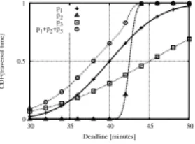
We now turn to define our routing algorithm, called ON-TIME, which aims at solving the on-time delivery problem. ON-TIMEfinds, in general, different paths for different values of (relative) deadline tstop−tstart. For example, Fig. 5 compares the Cumulative
Distribution Functions (CDF) for the delivery times of 3 different paths, for a given
0 0.5 1 30 35 40 45 50 CDF(traversal time) Deadline [minutes] p1 p2 p3 p1+p2+p3
Figure 5: Delivery probability CDFs of three disjoint paths P1, P2and P3, connecting a
source and a destination with different traversal times and without transmission failures (pf = 0). Path P1 has the lowest expected traversal time; the variance of P2is the
smallest, while P3’s variance is the largest. P1, P2and P3are respectively the optimal
paths computed by ON-TIMEfor deadlines between 34 and 43 minutes, larger than 43
minutes, and shorter than 34 minutes. The curve labeled P1+ P2+ P3 corresponds
to the success probability obtained by a multi-copy approach exploiting all the three paths.
source-destination pair and no transmission failures (pf = 0). In this case, ON-TIME
chooses one of the three paths depending on the given deadline. Nevertheless, the larger the deadline, the larger the resulting on-time delivery probability is.
ON-TIMEworks by first determining a potentially good path between the source to the destination (for example, that with the minimum expected traversal time), and eval-uating its on-time delivery probability. This can be done by performing a (numerical)
convolutionof the different random variables distributions along the path, yielding the
end-to-end traversal time distribution. By this distribution, it is then easy to calculate (using the corresponding CDF) the delivery probability by the deadline.
Then, the algorithm proceeds by exploring the graph through a breadth-first search, looking for paths with a higher on-time delivery probability. A pruning mechanism avoids the need to determine and evaluate all the paths. By the associativity of the convolution operator and the fact that our random variables are all non-negatives, for
any path P and any prefix P′ of P, Pr{tr(P) ≤ t} ≤ Pr{tr(P′) ≤ t}. Thus, we
can perform hop-by-hop convolution and compute, for each resulting distribution, the probability that the weight (that is, traversal time) of this path’s prefix is less than tstop− tstart; if the probability is smaller than that of the current best path, there is
no need to consider the rest of the path. From a practical point of view, working with a real transportation network, this simple pruning mechanism significantly reduces the number of paths to be considered, even if theoretically we may have a factorial number of paths to explore.
In our implementation, we have introduced some other simplifications, which re-duce the computation time, but, at the same time, may lead to suboptimal paths. First, we have introduced a limit h of the exploration depth during the search. Given h as a constant, the algorithm is then guaranteed to run in polynomial time. We observe that upon termination, we may be able to say if the algorithm has selected the optimal path or there may be a better one. In fact, when we stop, if there is still some path prefix of length not larger than h such that the pruning mechanism cannot discard it, then there could be a longer path with higher on-time delivery probability. But if this is not the case, then the current best candidate is actually the optimal path. In our experiments on Turin transportation network, h = 8 was enough to find all the best paths. Although this value may change for other networks, we except that it will remain a relatively
small constant. Note that a suitable h for each network can be found by conducting experiments similar to ours.
A second simplification is that we restrict the set of eligible paths such that each line can be used only in consecutive edges. This prevents the algorithm to explore paths using line ℓ1then line ℓ2, and then again line ℓ1. We expect that these paths have
normally worse performance than those where data message just remains on line ℓ1.
Finally, we have avoided the computation burden of performing numerical con-volution by assuming that the end-to-end traversal time, which is a sum of indepen-dent random variables, can be approximated by a normal distribution. In this case, it is sufficient to take into account the mean and the variance of each edge weight, conditioned on the fact that it is finite (respectively, µe = E[we|we<∞] and σe2 =
V ar[we|we<∞]), and the probability that the edge weight is finite (denoted by pe).
Then, the CDF of the traversal time of path P is equal to the CDF of a normal
dis-tribution with mean Pe∈Pµe and variance Pe∈Pσ
2
e, multiplied by a scaling factor
Q
e∈Ppe. In the case of travel edges, average and variance of tt(l, s, s
′) can be
mea-sured directly on the traces. In the case of travel-switch edges, we have to also to evaluate the average and variance of wt(ℓ, s, k) using the first three moments of the in-terarrival times of the line ℓ buses to stop s (which can be also measured on the traces) and some basic Palm calculus. For example, assuming perfect periodic bus arrivals with period δ and failure probability pf, E[wt(ℓ, s, k)] = δ(1/2 + pf/(1 − pf)) and
E[wt(ℓ, s, k)2] = δ2(1/3 + 2p
f/(1 − pf)2). Note that these values can be computed
for the specific arrival process observed in bus traces.
In what follows, we evaluate the performance of ON-TIME for different source-destination pairs under similar kind of deadlines. If we had fixed a given deadline for all the pairs, then this deadline could be unfeasible for some of them (in the sense that there is no way to deliver the message by this deadline, e.g. if the deadline is smaller than the time a vehicle would take to move from the source to the destination), and trivially satisfiable for other pairs (many different paths would deliver with probability almost one). For this reason, given a source ss, a destination sdand a real value x ∈ [0, 100],
let φ(x, ss, sd) be the deadline tstopfor which the on-time delivery probability of the
path from ssto sdwith minimum expected traversal time is x% (assuming pf = 0). We
denote by ON-TIME(x) the on-time routing algorithm where the deadline is set equal to φ(x, ss, sd) for every source-destination pair (ss, sd). Intuitively, the smaller x is,
the “shorter” the deadlines are considered, where “short” is in relation to the expected traversal time from ssto sdand not in an absolute sense.
4.3
Other Routing Approaches
Although the algorithm we described is optimal under our model assumptions, we also consider sub-optimal but simpler heuristics.
The most intuitive approach (denoted as MIN-DELAY) is to route in Gslalong the
path whose expected traversal time is minimal. Note that MIN-DELAYis equivalent to ON-TIME(50) under the Gaussian assumption on the distribution of the traversal time. Fig. 5 shows that path P1, found by MIN-DELAY, does not always correspond to the
highest on-time delivery probability. On the other hand, MIN-DELAYis computation-ally attractive, because the path with the least expected traversal time can be easily computed with Dijkstra’s algorithm (by linearity of expectation). In Sec. 5, we com-pare our optimal algorithm to this sub-optimal heuristic and show that it often suffices to use this simple approach.
A second algorithm, MAX-PROB, selects the path that maximizes the delivery probability on an infinite time-horizon. Also this path can be determined running Di-jkstra’s algorithm on the line-stop graph with edge weights equal to − log(pe). MAX
-PROBand ON-TIMEtend to select the same path, for low transmission success proba-bilities, as shown at the end of Sec. 5.
Another approach, denoted MIN-HEADWAY, tries to minimize the sum of all lines headways along a path [38], thus preferring frequent lines over infrequent ones; it was proposed originally for bus-to-bus communications. In Sec. 5, we show that it has the worse performance in our settings among all the different algorithms.
4.4
Extension to Multi-Copy Routing
As shown in the toy-case of Fig. 5, using a multi-copy scheme (the curve labeled “P1 + P2+ P3”) to exploit several paths simultaneously increases the on-time
de-livery probability to deliver the data within the deadline. In this specific example, path P2becomes “useful” only for large deadlines, whereas P3is “useful” for any deadline.
For multi-copy scheme, we consider only non-flooding algorithms, such that at most k copies of the packets are made throughout the execution (otherwise, an optimal flooding scheme can copy the data whenever there is a contact, namely in an epidemic
manner, thus achieving the best possible delivery probability).
We propose a greedy Multi-Copy algorithm for on-time routing, denoted simply as MC-ONTIME. It computes the on-time delivery probability of all paths in isolation and choose the k best paths (without considering the interaction between them). This can be easily implemented by saving the best k paths while enumerating all possible paths as in ON-TIME. Moreover, our pruning mechanism is changed accordingly to consider the k-th best value discovered so far (rather the maximum value as in the single-copy settings)5.
However, since our algorithm works in a greedy manner, it does not consider the interaction between the paths, and more specifically the gain in probability over previously-selected paths (which can be very small in case the paths overlaps). This leads to a theoretical performance degradation with respect to an optimal, infeasible algorithm that considers the joint-probability over all sets of paths. The following theorem, whose proof is in Appendix F, provides tight bounds on this performance degradation:
Theorem 1. TheMC-ONTIMEalgorithm always achieves at least1/k of the on-time
delivery probability of an optimalk multi-copy algorithm. In addition, there is a valid
transportation graph for whichMC-ONTIMEachieves at most (1−ε)k1 of the on-time delivery probability of an optimalk multi-copy algorithm, for arbitrarily small ε > 0. The performance degradation is mainly due to path overlapping; consider two paths with high success probability that differ only in one edge: MC-ONTIME will choose both paths, while, in fact, the marginal gain in choosing the second path is small. Thus, we consider also an algorithm that ensures that the paths are disjoint. Namely,
the MC-ONTIME-DISJOINT algorithm iteratively chooses the path with the highest
on-time delivery probability, among all paths from source to destination whose corre-sponding lines are not used by any previously-selected path. However, we show that
the worst-case performance of MC-ONTIME-DISJOINTis the same as MC-ONTIME.
5When comparing to the heuristics of Sec. 4.3, we can similarly get the k paths with minimal expected
traversal time, total headway or maximal success probability.
0.01 0.1 1
0 10 20 30 40 50 60
P(W>w)
Time interval [min]
Figure 6: Complementary CDF of the critical time window W guaranteeing on-time delivery probability ∈ [0.1, 0.9] for the minimum expected traversal-time path. Our simulations clearly show that the MC-ONTIMEis superior in practice, and there-fore this is the multi-copy routing algorithm we consider in the sequel.6
5
Performance Evaluation
We consider a set of 180 source-destination (ss−sd) stop pairs; in the first 90 pairs
both the source and the destination have been chosen uniformly at random in the entire metropolitan area; in the second 90 pairs, the source ssis located in a main
transporta-tion hub within the city center (close to the main train statransporta-tion), and all the destinatransporta-tions sdare chosen uniformly at random. We generate a set of 100 traces with the parameters
obtained by the statistical analysis, covering all 250 lines for the four hours available from the schedule. In addition, we have developed a simulator that computes the de-livery probability of each path by averaging across these 100 traces; note that the one day real-life trace alone would not be enough to compute this probability with any accuracy. Data is assumed to be available at the source stop at 7 AM.
For these 180 ss−sdpairs, we start to evaluate the size of the “critical” time
win-dowdefined as W = φ(90) − φ(10): this is the amplitude of the interval of
“reason-able” deadlines for which MIN-DELAYand ON-TIME(50) achieve delivery probability in [0.1, 0.9]; intuitively, when considering any deadline outside this critical time win-dow, one is either likely to fail or to succeed, and the randomness in the transportation system does not play a major factor. Fig. 6 shows the inverse CDF of W , considering the whole set of 180 pairs. For more than 90% of ss−sdpairs, the windows is larger
than ten minutes and for more than 17% of them, it is even larger than 20 minutes. The maximum critical window size we observed is 67 minutes. As a consequence, the time window for which the deadline plays an important role on the delivery probability cannot be neglected for most of these 180 ss−sdpairs.
Then, for all 180 pairs and for all 100 traces, we evaluate the optimal paths found by the ON-TIMEalgorithm and compare their theoretical on-time delivery probability with the empirical one determined by simulations. We found a reasonable agreement, even if not perfect in absolute values since in our model we assumed that line fre-quency and headway distribution do not change over time or between station along the same line; in real-life, there are small fluctuations in these values. In addition, while generating the synthetic traces, we introduce some inhomogeneity in the travel time
6MC-ONTIME-DISJOINTand MC-ONTIMEare two extremes as for the amount of overlapping between
the paths. In our future research, we plan to look also on hybrid heuristics with strict bounds on the number of overlapping edges. While these variants yield the same1
kworst-case approximation, they might be proved
superior in real-life traces.
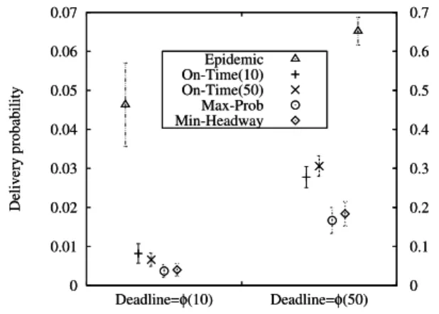
0 0.01 0.02 0.03 0.04 0.05 0.06 0.07 0 0.1 0.2 0.3 0.4 0.5 0.6 0.7 Delivery probability Deadline=φ(10) Deadline=φ(50) Epidemic On-Time(10) On-Time(50) Max-Prob Min-Headway 0 0.01 0.02 0.03 0.04 0.05 0.06 0.07 0 0.1 0.2 0.3 0.4 0.5 0.6 0.7 Delivery probability Deadline=φ(10) Deadline=φ(50) Epidemic On-Time(10) On-Time(50) Max-Prob Min-Headway
Figure 7: Delivery probability (average and 90% confidence interval) for two deadlines and different routing algorithms, for reliable transmission (pf = 0). MIN-DELAYis
the same as ON-TIME(50).
distribution to ensure that buses maintain their order; our model, on the other hand, considers homogeneous travel time distribution that depends only on the scheduled travel time (See Appendix C).
We start to compare the performance of the algorithms defined in Sec. 4—namely,
MIN-DELAY, ON-TIME, MAX-PROBand MIN-HEADWAY—with the EPIDEMIC
al-gorithm that floods the network by taking advantage of all the possible contacts (and therefore making very large number of copies). We first assume that transmissions are reliable, i.e. pf = 0. We evaluate the actual on-time delivery probability of the best
path obtained by each algorithm; for each pair ss−sd, we set the deadline to φ(x) for
different values of x, and we compute the 90% confidence interval of the delivery prob-ability considering all the possible 180 pairs. Due to the lack of space, we will report the results only for x = 10 (“short deadline”) and x = 50 (“average deadline”), since these cases are representative.
Fig. 7 compares the delivery probability of the different algorithms for the two deadlines. The gain on the delivery probability of EPIDEMICwith respect to all the other single-copy algorithms decreases as the deadline increases: the factor of gain is more than 5 for deadline φ(10) and around 2-3 for deadline φ(50). Indeed, when the deadline is large enough, outside the critical time window, just one copy of the data is enough, independently from the actual path found by the specific routing algorithm; in
such a case, EPIDEMICdoes not introduce any gain in terms of performance, and the
cost in terms of copies and transmissions is prohibitive (we observed on average more than 600 copies for φ(10) and more than 900 copies for φ(50)) than the single-copy algorithms, for which the number of transmissions for each data is on average 5.5, and always less than 12.
ON-TIME(10) and ON-TIME(50) obtain the maximum delivery probability respec-tively, for deadline φ(10) and φ(50), as expected. But comparing the corresponding confidence intervals, they behave almost the same. A somewhat surprising results is that in many cases (121 out of 180) ON-TIME(10) performs exactly as ON-TIME(50) (or, equivalently, as MIN-DELAY). In such cases, we verified by direct inspection that ON-TIME(10) and ON-TIME(50) select exactly the same optimal path.
0 0.05 0.1 0.15 0.2 0.25 0.3 0.35 Delivery probability Min-Delay Max-Prob pf=0.0 pf=0.1 pf=0.3 pf=0.5
Figure 8: Delivery probability (average and 90% confidence interval) for MIN-DELAY (i.e., ON-TIME(50)) and MAX-PROBfor deadline φ(50) and for different values of transmission failure probability pf.
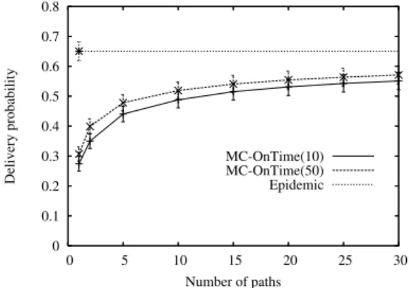
0 0.1 0.2 0.3 0.4 0.5 0.6 0.7 0.8 0 5 10 15 20 25 30 Delivery probability Number of paths MC-OnTime(10) MC-OnTime(50) Epidemic
Figure 9: Delivery probability (average and 90% confidence interval) vs. number of paths for deadline φ(50) and for multi-copy routing and no transmission failures (pf =
0).
These results have been confirmed also for other deadlines: ON-TIME(50) usually selects the best path computed by ON-TIME(x) for the deadline φ(x). Recall the ex-ample in Fig. 5, showing that the best path may depend on the deadline. While it is possible in a general setting, our experiments lead us to conclude that these cases are very rare in a real transportation system. Thus, one can choose the path solely on the basis of the minimum expected travel time (that is, the simple MIN-DELAYalgorithm), making it redundant to run the complex optimal algorithm ON-TIME.
We now investigate the effect of transmission failures. Fig. 8 shows the deliv-ery probability for different values of transmission failure probability pf. When pf
increases, MIN-DELAYbehaves very similarly to MAX-PROB; we expect that MAX -PROBbecomes very efficient when the transmission failures are high, since the best
policy must minimize the number of transmissions. Hence, both MIN-DELAY and
MAX-PROBappear to behave very efficiently for large pf.
We turn now to deal with multi-copy settings. Fig. 9 shows the performance of
the MC-ONTIME policy, applied to the first best pre-computed paths found by each
routing algorithm in all the considered 180 source-destination pairs, assuming reliable transmissions (pf=0). For deadline φ(50), ON-TIMEwith one copy reaches a delivery
probability which is slightly less than half (more precisely, 42% and 47%) than the
epi-demic case, and few copies of MC-ONTIMEimprove the performance significantly by
a factor 1.7-1.9. Yet, after 10 copies we observe only a negligible improvement. This is partially due to the fact that MC-ONTIMEexploits a given sequence of paths provided by the algorithms, whose internal “diversity” among the paths is limited. Furthermore, EPIDEMIC exploits low-probability paths that are efficient just for the specific trace instance considered in each simulation run; since the number of these low-probability paths can be very large, due to the redundant connectivity of the bus transportation system metropolitan area, there might be a high probability that at least one of them will be used to deliver to the destination. Note that the cost in terms of transmissions and copies for EPIDEMIC(on average, more than 900) is two order of magnitude larger than the multicopy approach using a pre-selected subset of 10 paths.
6
Conclusions
This paper lays the foundations for a framework to analyze bus-based networks, where communication is between the mobile buses and the stops along their trajectories. Through a statistical analysis of traces, taken from a real transportation system of a large urban area, we were able to obtain a succinct stochastic graph representation of the system, and to devise routing algorithms on this graph. In addition, we were able to develop a synthetic trace generator, which in turn allowed us to perform an extensive simulation study, verifying the performance of our proposed algorithms.
An important outcome of this study is that, although different from the optimal
but computationally-intensive algorithm, the simple MIN-DELAYalgorithm achieves
excellent results in term of success probability for any reasonable deadline. In addition, we show that increasing the number of data copies beyond 10 does not provide any meaningful boost in performance.
As final comment, we note that our model can be extended to bus-bus communica-tions by introducing some virtual stops, located in correspondence to possible physical contact points between two different lines. By appropriate choice of weights on the corresponding edges (e.g., no waiting time and high failure probability), one can cap-ture the nacap-ture of this kind of communication as well. The main challenge, left for future research, is to locate the physical contact points and to bound their number so that the running times of the algorithms remain feasible.
A
Comparison of Bus-Bus vs Bus-Stop Communications
For the scenario under consideration, where a rather large set of buses roam around a city, the prior work has primarily focused on transfer of messages through opportunistic links that are formed when two buses come within the proximity of each other. Apart from the physical layer restrictions such as scattering, slow and fast fading, this ap-proach may cause problems because of insufficient contact time. Burgess et al. show that the contact duration between two mobile nodes can be very short to prevent the transfer of all the messages the nodes maintain in their buffers [10].
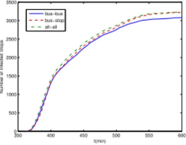
350 400 450 500 550 600 0 500 1000 1500 2000 2500 3000 3500 t(min)
Number of Infected Stops
bus−bus bus−stop all−all
Figure 10: Comparison of Epidemic Routing with bus-bus & bus-stop communications We now evaluate bus-bus and bus-stop communication paragidms without taking these effects into account. Instead, we look at how fast a message propogates in a transportation network using these two paradigms. Considering the schedule informa-tion for the buses as well as the locainforma-tion informainforma-tion of the stops, we have extracted the times when any two buses are supposed to form a link based on the schedule. Here, we used the common disc model where if the distance between two nodes are smaller than a threshold value at a given time, they are neighbors and one can transmit data to the other.
In Fig. 10, we compare the epidemic routing schemes with bus-bus and bus-stop communication approaches. In bus-bus approach, a bus can receive a packet only from another bus, i.e. only a bus can infect another bus. Stops are infected by buses but a stop can not infect the buses. In bus-stop approach on the other hand, the buses can only be infected by stops and vice versa. In all-all communcations, all the contact opportunities (both bus-stop and bus-bus) are utilized. Here we assumed, a packet starts at a busy bus stop that serves many lines and epidemic routing proceeds without a particular destination stop. We evaluate how the number of infected stops increase over time. In bus-bus case, the source stop only infects the first encountered bus. The results show that bus-stop is at least as effective as bus-bus communications to spread the information. In fact, as the time progresses, the number of infected stops become identical with the all-all case whereas bus-bus communcations may not diffuse the message to all the stops that bus-stop communications can.
Remember that this evaluation assumes perfect physical and link layers, and does not consider the effects of short contact duration, scattering, etc. In bus-stop commu-nications, such effects are mitigated because the wireless links are formed between two stationary nodes as opposed to mobile nodes. The time in which passengers board and alight is much larger than the time two moving bus enter and exit each other’s communication range.
B
Bus Mobility Models in Transportation
This investigation of the transportation literature is mainly based on the overviews in [12, 4].
Some works provide probability distribution for arrival time or lateness or delay, based on empirical studies (e.g. [43, 42, 19, 39, 40] or on model simplification (e.g., [1, 24]). Most studies prefer to use a skewed distribution since it is more likely to be behind schedule than ahead. Lognormal or gamma random variables are the most common assumptions (see the summary table in [12]).
About the statistical dependency of these quantities, contrasting effects hold. In general once a bus with low headway is late at a given stop, it is difficult to recover its lateness. In fact, for lines with low headways, passengers usually do not regulate their arrival on the basis of the schedule. Hence, passenger arrival can be assumed to be a Poisson process. When a bus is late, the longer waiting time at following stops causes an increase in the number of passengers who board (and later alight) resulting in longer dwell times and higher and higher delay en-route. Therefore, lateness and delay are positively correlated in such cases: high lateness at a stop results in increased delay over the subsequent segment [43]. This phenomenon does not always occur on buses with higher headway. In fact, passengers now tend to arrive just before the scheduled departure time of desired bus. Hence, late buses do not board significantly more passengers than on-time buses. Furthermore, since higher headway buses often have slack built into their schedule, there is opportunity to recover some of the lost time [23]. Penalties to drivers for being excessively late encourage them to catch up to the schedule. Thus, the delay in a segment is negatively correlated with the lateness at the start of the segment. Because of these two phenomena, the delay on a bus line segment can either be negatively or positively correlated with the lateness at the start of the segment, depending in large part on the line headway. Moreover, we observe that the lateness of a bus also has consequences on following buses on the same line and direction. A late bus boards more passengers, and so it leaves less of them for the following bus. This effect would lead to a negative correlation between the lateness of consecutive buses. At the same time in many cases transport agency policies or traffic conditions make overtaking impossible or quite rare. Hence a bus that is significantly late would cause also the consecutive ones to be late.
Regarding dwell time, this can be a significant part of the total service time (up to 16% of the total service time according to [4]). This time clearly depends on the number of passengers boarding and alighting (empirical formulas are proposed in [27] and [20]), but also on the crowding, fare types [19], payment modalities, bus design (separate/common doors for boarding and alighting), mode (i.e. bus or metro lines) and service type7 [41]. Also, the contribution of dwell time to lateness correlation is not
immediate. For example a large dwell time can be due to a large number of passengers boarding or alighting. In the first case the alighting at following stops will in general large, in the second will be small.
C
Generation of Tunable Synthetic Traces
In this section, we describe the evolution of building the synthetic traces, from the scheduled raw traces which we could have for a public bus transportation from the available schedules on their website.
Based on the empirical study and after performing a deep analysis on the GTT
(Gruppo Torinese Trasporti)bus traces for a subset of bus lines, we could notice that
lateness at following stops are highly correlated, where lateness at the initial stop, i.e. l(s0) following the notion in Sec. 3, is triangularly distributed with support between
[-2,+2] in minutes. On the other hand, it seems that the distribution of actual travel time is a lognormal, where the distribution parameters vary according to the scheduled travel time, ST T . This observation complies with previous studies on the travel time in
7Service type can be rapid, limited, local, or combined depending on the vehicle speed, and the distance
between consecutive stops.
transportation networks (See Appendix B). The following formulas are used to evaluate the mean and the variance of the travel time, denoted by MT T and VT T, respectively.
MT T = 0.7(ST T + 0.5) (2)
VT T =
M2
T T
4 (3)
The actual arrival time of a vehicle v at stop sk is given in (1). The arrival time
at s0, t(v, s0) is the summation of the scheduled arrival time and the lateness at that
stop, l(s0). While the arrival time at a following stop is the summation of actual arrival
time at the previous stop and the actual travel time calculated based on the scheduled travel time, following the predefined lognormal distribution. Here the travel times and the lateness of the bus at the initial stop, l(s0) are independently generated. The actual
arrival time at stop skis given by:
t(v, sk) =
(
τk+ l(sk) for k = 0
t(v, sk−1) + tt(v, sk−1, ki) for i > 1
.
Another observation from the real life traces is that the scheduled travel time for a vehicle between two consecutive stops is always less than 6 minutesAlthough with low probability, the random variable generator can produce numbers that are greater than this value. In this case, we truncate the output of the generator to 6 minutes.
During the evolution of generating the synthetic traces and each time we calculate the actual arrival time, we should check if such actual travel time will cause a negative headway. In other words, one vehicle can overtake the previous vehicle on the same line, a phenomenon not observed in the real life traces. In this case, we generate an-other new independent travel time and re-evaluate the actual arrival time again while keep considering the negative headway effect. At the same time, we maintain these unused values in a queue. Before we generate a random value from a particular dis-tribution, we check the queue if there is random variable in the queue generated from this distribution. If the value in the queue does not cause negative headway, it is used without generating a new random variable. At the end of each run, we see that there may be some values in the queue; however, their number is significantly less than the total number of values generated. Hence, we maintain the empirical distribution of the travel time.
D
Bus stations aggregation
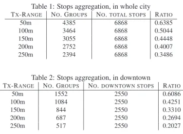
In this section, we show how to aggregate the bus stations (stops) into groups. The goal behind aggregation is to reduce the number of attached wireless boxes at the stops. the stops physical location and the effective coverage range of the wireless boxes are the main parameters of the aggregation process. the coverage range is assumed to be homogeneous along all the stops. With a given coverage range find the stop that has the maximum number of neighbors in its range, this stop will be attached to a wireless box, the stop and its neighbor/s are considered to be in one group, we follow the same procedure to determine other group/s after neglecting the set of stops in the earlier found group/s.
Different transmission ranges are considered 50, 100, 150, 200 and 250 meters, table 1 shows the ratio of stops attached to the wireless boxes to the total number of


![Figure 6: Complementary CDF of the critical time window W guaranteeing on-time delivery probability ∈ [0.1, 0.9] for the minimum expected traversal-time path.](https://thumb-eu.123doks.com/thumbv2/123doknet/12767049.360132/19.918.356.530.147.272/figure-complementary-critical-guaranteeing-delivery-probability-expected-traversal.webp)