HAL Id: hal-02070777
https://hal.archives-ouvertes.fr/hal-02070777
Submitted on 18 Mar 2019
HAL is a multi-disciplinary open access
archive for the deposit and dissemination of sci-entific research documents, whether they are pub-lished or not. The documents may come from teaching and research institutions in France or abroad, or from public or private research centers.
L’archive ouverte pluridisciplinaire HAL, est destinée au dépôt et à la diffusion de documents scientifiques de niveau recherche, publiés ou non, émanant des établissements d’enseignement et de recherche français ou étrangers, des laboratoires publics ou privés.
Acoustical characterisation and monitoring of
microbubble clouds
Lilian d’Hondt, Matthieu Cavaro, Cédric Payan, Serge Mensah
To cite this version:
Lilian d’Hondt, Matthieu Cavaro, Cédric Payan, Serge Mensah. Acoustical characterisation and monitoring of microbubble clouds. Ultrasonics, Elsevier, 2019, �10.1016/j.ultras.2019.03.009�. �hal-02070777�
Accepted Manuscript
Acoustical characterisation and monitoring of microbubble clouds Lilian D'Hondt, Matthieu Cavaro, Cédric Payan, Serge Mensah
PII: S0041-624X(18)30700-5
DOI: https://doi.org/10.1016/j.ultras.2019.03.009
Reference: ULTRAS 5910
To appear in: Ultrasonics
Received Date: 15 October 2018
Revised Date: 8 March 2019
Accepted Date: 12 March 2019
Please cite this article as: L. D'Hondt, M. Cavaro, C. Payan, S. Mensah, Acoustical characterisation and monitoring of microbubble clouds, Ultrasonics (2019), doi: https://doi.org/10.1016/j.ultras.2019.03.009
This is a PDF file of an unedited manuscript that has been accepted for publication. As a service to our customers we are providing this early version of the manuscript. The manuscript will undergo copyediting, typesetting, and review of the resulting proof before it is published in its final form. Please note that during the production process errors may be discovered which could affect the content, and all legal disclaimers that apply to the journal pertain.
Acoustical characterisation and monitoring of
microbubble clouds
Lilian D’Hondt†,††
, Matthieu Cavaro†
, Cédric Payan††
and Serge Mensah††
† CEA – DEN/CAD/DTN/STCP/LISM – Bat 202 – 13108 St-Paul-lez-Durance - France ††Aix-Marseille Univ, CNRS, Centrale Marseille, LMA, Marseille, France
Contact: dhondt.lilian@gmail.com; matthieu.cavaro@cea.fr
Argon microbubbles will exist in the primary sodium of the next generation of sodium-cooled fast reactors (SFR). Due to its opacity, acoustic methods will be used for the in-service inspection in these reactors, but the presence of such bubbles will greatly affect ultrasonic wave propagation. Moreover, these bubbles can lead to the formation of gas pockets in the reactor and impact cavitation and boiling phenomena. It is therefore necessary to characterise what is called the ‘microbubble cloud’ by providing the volume fraction and the bubble size distribution. Safety requirements in this field call for robust inspection methods based on very few assumptions about the bubble populations. The objective of this study is to assess the performance of spectroscopic methods in the presence of bubbles with high polydispersity and to monitor an evolving cloud of microbubbles. The histogram and void fractions were estimated according to the regularised inversion of the complex wave number’s integral equation. To reduce the need for prior information on the bubble cloud, a specific procedure was used to estimate the maximum radius of the population. The results are presented on the basis of the experimental data obtained and then compared with optical measurements.
1 I
NTRODUCTIONThere will be a normal, continuous microbubble cloud in the primary system of the Generation IV sodium-cooled fast reactor (SFR) prototype called ASTRID1, due to the existence of the argon gas plenum. Although there is no direct characterisation of the bubble cloud in SFRs, indirect measurements and existing calculation codes, such as VIBUL [1] - developed in the 90s at the CEA - give bubble sizes ranging from a few µm to a few tens of µm for a void fraction about . As sodium is an opaque
liquid metal, visual inspection of the reactor is impossible. Consequently, ultrasonic inspection methods are preferred, for example, to check the presence and position of some components such as fuel sub-assemblies, or to monitor the structural health of components (SHM). For this purpose, the telemetric approaches generally used may be severely altered if the speed of sound of the bubbly mixture is modified by the presence of bubbles in the sodium. Moreover, microbubbles have an
1
Advanced Sodium Technological Reactor for Industrial Demonstration
impact on cavitation and boiling, acting as germs which could also lead to the formation of gas pockets in the reactor. For these reasons, safety requires the characterisation of this microbubble cloud using as few assumptions as possible [2].
In this paper, the term ‘characterisation’ refers to the estimation of the void fraction and the bubble radius
distribution. Interest in bubbly liquid
characterisation is not new; Medwin [3], [4] covered this issue in 1970 when analysing the bubble population on top of oceans. An analytic expression was used to estimate the bubble radius distribution from attenuation measurements. Only the resonant bubbles were taken into account. This method has since been improved by Caruthers and Elmore [5], [6] who implemented an iterative procedure to overcome the approximations made by Medwin. Commander and Moritz [7] then showed that the non-resonant bubbles also needed to be taken into account to produce more reliable results. This implies the use of numerical methods to solve the integral equation that links the bubble distribution to their acoustic properties. The first numeric approach was proposed by Commander and Moritz [8] and was later improved by the Dynaflow laboratory. Duraiswami et al. [9]–[13]
considered the contribution of velocity
measurements in the inversion process. Leighton [14] suggested the use the “L-curve” method to determine the regularisation parameter used to optimise the inversion process.
However, the radius range was always fixed prior to the measurements in all the papers listed above. This is in contradiction with an ‘assumption-free approach’. Moreover, the bubble size histograms given in the literature have poor resolution (bin size ) and the void fractions are generally not estimated. Furthermore, the results are not systematically compared against alternative measurements.
This paper describes a method that is able to continuously monitor the microbubble cloud in operational SFR conditions. It is based on the spectroscopic measurement of attenuation and sound speed with no prior information about the
bubble size interval to obtain the void fraction and bubble size distribution. The experimental acoustic results of this method have been compared with optical measurements, thus providing both the bubble size distribution and void fraction.
The theoretical background is presented in the first section. The inversion procedure is then detailed and validated against two kinds of bubble distributions. Next, the experimental bench designed to reproduce - in water – the SFR operational conditions is described. Finally, the method is validated experimentally for a stationary distribution and for the continuous monitoring of a varying bubble cloud.
2 T
HEORETICAL BACKGROUNDThe propagation of a pressure wave in a bubbly liquid can be described by the wave equation derived by Commander and Prosperetti [15]. This equation, deduced from the linearisation of the Keller-Miksis equation leads to the expression of the wave number :
(1)
where
is the wave’s pulsation;
is the
sound speed in pure water (without bubbles);
is the number of bubbles per unit volume
with a radius between and ;
is the
resonance pulsation of a bubble with a radius
, and is the damping coefficient associated
with the thermal, viscous and radiative
processes.
The sound speed and of the effective medium can be calculated on the basis of Eq. (1). Let and be the dimensionless velocity and attenuation coefficients:
( 2)
where
is the wave number in pure liquid.
Then:
3) (
Figure 1: Experimental distribution. Void fraction:
An experimental distribution was used in this section to describe the concepts and the method (Figure 1). This distribution was obtained using the optical image processing described in Section 3.2.3. Using equation (3), the dispersion curves corresponding to this bubble size distribution have been plotted in Figure 2.
Figure 2: Dispersion curves calculated using Eq. (3)
Determining the characteristics of the bubble cloud from spectral measurements implies an inversion of Eq. (1). By separating the complex wave number into real and imaginary parts, Fredholm equations of the first kind can be derived [11], which leads to:
D’Hondt et al., p.3 ( 4)
where is the bubble size distribution. The
expressions of the kernels
are as
follows:
( 5)According to Duraiswami [11], the -based expression provides more robust estimations. In all cases, we need to invert an equation of the form:
(
6) where is greater than the bubble cloud’s maximum radius. This equation discretises into:
(
7)
where
and
an
matrix whose coefficients are
:
(
8) is the linear B-spline [16]. The number of
measurements is equal to , the number of radius classes of the bubble size histogram.
As problem (7) is ill-conditioned, a Tikhonov regularisation procedure was introduced [17], [18] and led to the solution:
(
9) Under the positive and finiteness constraints:
10) (
is the regularisation parameter. It must be correctly adjusted and is a tridiagonal matrix: . is an a priori estimation of the solution that can be set to zero if no information is available. Here, . This equation can be solved using a least-square algorithm. Moreover, if the void fraction can be
estimated separately, for example through Wood’s model using low-frequency acoustic velocity measurements [19], this value can be introduced into the set of constraints.
Figure 3: Typical L-curve obtained using the scripts by Hansen [18]
In order to obtain a good estimation of the bubble size distributions, the regularisation parameter was adjusted using the L-curve method described by Hansen [17]. The L-curve plots
versus the residual norm at
different . On the one hand, if the regularisation parameter is too small, the residual norm is reduced, but the solution norm may still be large since the problem is ill-conditioned. On the other hand, if the regularisation is significant, the solution is dominated by regularisation errors. Hansen has shown, with respect to the so-called Discrete Picard Condition, that a physical approximation of exists. In this case, the L-curve is indeed “L-shaped” and the optimal regularisation parameter lies at its corner (Figure 3).
3 M
ATERIALS AND METHOD3.1 Determining the maximum radius of integration
Intuitively, the maximum radius of integration
(Eq. (6)) should be greater than the radius of
the largest bubble in the cloud. However, it should not be too large to avoid unnecessary classes. In order to determine , a “L-surface” was built to correspond to the surface spanned by the L-curves when the maximum radius varies (Figure 4).
Figure 4: L-surface for an experimental bubble size distribution. The red line plots the L-curve with the selected .
When , the radius range is incoherent with the dispersion curves, the L-curves therefore are not clearly L-shaped and they do not provide a strong curvature (at the
corner) as a function of . Conversely,
when , the radius histogram will have excessively larges classes and the solution will be ‘blurred’. The optimal maximum radius is then the smallest of those providing a sharp L-curve with an almost constant solution norm for large . Equation (9) was then solved using the regularisation parameter proposed by this L-curve.
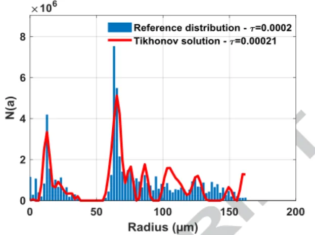
Figure 5: A reference distribution obtained optically (blue bars) and the recovered solution (red line) using eq. (9)
This has been simulated based on an optically characterised experimental distribution (Figure 1). The L-surface provided a good estimation of the bubble cloud’s maximum radius. The proposed maximum radius is , which is in agreement with the distribution. Based on the optical data, acoustic dispersion curves were assessed using Eq. (3) and a small amount of Gaussian noise was added ( to the measurement vector to mimic experimental noise. The result of the inversion is shown in Figure 5.
Figure 6: A reference distribution obtained experimentally (blue bars) and the recovered solution (red line) using eq. (9)
This procedure is also relevant for more exotic distributions such as the one shown in Figure 6 which was characterised optically. In this case, the acoustical inversion was not possible because our transducers are inefficient at the low frequencies required to characterise large bubbles ( ). Nevertheless, the use of synthetic data shows that the inversion procedure remains possible albeit difficult. The L-surface (Figure 7) proposes a maximum radius of 162 µm, which corresponds to the radius of the largest bubble.
Figure 7: L-surface for a bi-modal experimental bubble size distribution. The red line plots the L-curve with the selected . Hansen shows that when the solution is too smooth, i.e. it is dominated
by the first few singulars values, the regularisation parameter corresponding to the L corner fails to correctly estimate the solution. This should not be the case for ‘standard’ distributions such as those expected in a reactor configuration. The relative error versus the
regularisation parameter is shown in (
D’Hondt et al., p.5
(11)
Figure 8: Relative errors for the experimental distribution. The red circle corresponds to the minimum error while the dashed line shows
the position of the regularisation parameter selected by the L-curve
This error analysis shows that the regularisation parameter selected by the L-surface does not correspond exactly to the optimal regularisation (which is the one that minimised the relative error). However, the error remains acceptable (around ). The main advantage is that the L-surface method provides a robust and systematic way to reach a good regularisation coefficient.
3.2 Experimental bench
Experimentations in liquid sodium should be performed with extreme care as sodium is highly reactive to air and water. Moreover, it is a strong reducing agent which implies using specific transducers designed to operate in such a chemical and thermal environment, e.g. the TUSHT [20]. However, as the acoustical properties of argon bubbles in liquid sodium – especially the impedance contrast – are similar to those of air bubbles in water (see Table 1), preliminary experiments were performed in water.
3.2.1 Bubble generation
Figure 9: 3D model of ACWABUL
In order to validate the inversion procedure detailed above, an experimental bench called ACWABUL (Acoustical Characterisation in WAter of BUbbLes) was manufactured at the CEA Cadarache centre to reproduce the required SFR operational conditions in water.
Table 1: Acoustical properties of argon bubbles in liquid sodium compared with those of air bubbles in water [21]–[24]
UNIT WATER/AIR 20°C/1 BAR SODIUM/ARGON 550°C / 1 BAR Massive thermal capacity of gas J/(kg.K) 1.01x10 3 520,4 Acoustical velocity in gas m.s -1 340 535 Acoustical velocity in liquid m.s -1 1481 2292 Gas compressibility factor - 0.9996 1.00025 Compressibility of the liquid Pa -1 4.4x10⁻¹⁰ 1.86x10⁻¹⁰ Thermal conductivity of gas W/(m.K) 0.026 0.0381 Acoustic
impedance of gas rayls 413 311 Acoustic
impedance of liquid rayls 1.5x10
6 1.9x10⁶ Gas density Kg.m-3 1.3 0.582 Liquid density Kg.m-3 1000 816 Surface tension parameter N.m -1 72.8x10⁻³ 151x10-3
Liquid viscosity Pa.s 10-3 0.2268x10⁻³
Acoustical attenuation w/o bubbles
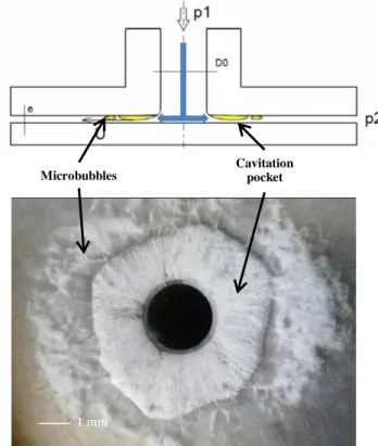
This bench consists of a 1m3 tank, saturator and injectors (Figure 9). Water is first air-saturated at 7 bar in the saturator (300L). It is then injected through specific injectors designed to induce air cavitation (Figure 10) thanks to radial divergence.
Saturator Injectors Tank
Figure 10: Geometry and image of the microbubble generator (courtesy of Ylec Consultants)
The induced rapid relaxation creates a cavitation pocket which collapses. As the water is over-saturated, stable microbubbles with radii of a few microns to few tens of microns still remain. This process makes it possible to generate clouds like those expected to be found in the reactor.
By varying the numbers of injectors opened and the feeding pump speed rotation, it is possible to adjust the void fraction from to . The resulting bubbles have a radius between and with a distribution approximately log-normal.
3.2.2 Acoustic measurements
To estimate the phase velocity and attenuation at every frequency of interest, transmission measurements were performed by sending two sets of monochromatic 10-cycles bursts. The first set was sent in bubble-free water while the second was sent in bubbly liquid. The bursts ( and ) were then compared with each other. The attenuation at the frequency was calculated using (12). The phase velocity at the same frequency was calculated using (13).
(12) (13)
where is the fast Fourier transform
of the signal
is the central frequency of the
burst; is the distance between the emitter
and the receiver; and
is the argument of
the complex function .
Figure 11: Image of the experimental set-up
To cover the entire frequency range of interest, two custom-made Imasonic® planar transducers (central freq. 250 kHz with an active diameter of 46 mm) were used for broadband measurements between 20 kHz and 400 kHz (Figure 11). The waveforms were generated using a Tektronix® AFG 3022B function generator digitised with a PicoScope® 4824. Both these devices were connected to a computer used to control the experiment through a dedicated Matlab® script. To avoid any non-linearities [25], the wave amplitudes were kept as low as possible.
3.2.3 Optical measurements
A BAUMER® TXG50-IP67 underwater camera with a VS-Technologies® telecentric lens
captured several images of the clouds
simultaneously with the acoustic measurements. The use of telecentric optics makes it possible to accurately measure the size of a bubble, as its size on the image does not depend on its position in space. However, the depth of field is very narrow, i.e. only few millimetres. Only bubbles with a blurring level below a pre-set level were selected. A dedicated algorithm [2] was then used to estimate the bubble size distribution and the void fraction (Figure 12). The void fraction was determined by measuring the blurring level on each bubble in order to deduce its distance from the focal plane of the camera (Figure 13) using a prior calibration of the optic device. This was used to estimate the volume of interest covered by the camera for each size of bubble. Camera Imasonic 250 kHz Imasonic 250 kHz LED panel Bubbles Microbubbles Cavitation pocket
D’Hondt et al., p.7
Figure 12: Video frame of the bubble cloud. The bubbles selected and sized are delineated by the red circles
It is worth pointing out that this camera underestimated the number of bubbles with a radius
due to the optics used.
Figure 13: Blur versus distance to the focal plane for different bubbles sizes
Figure 14 shows the void fraction obtained by this optical procedure compared with the one obtained by low-frequency velocity measurements, following the procedure described in another study [19]. The void fraction was modified by switching off a bubble injector at and then switching it on again at .
Figure 14: Void fraction estimated by the optical set-up and using sound speed measurements at low-frequency [19]
The optical and acoustic means provided coherent void fraction estimations. There was a small bias between the optical and acoustical estimations. It increased with the void fraction,
though remained within the measurement
uncertainties. This discrepancy may be due to the fact that the bubbles may become too close to each
other as increases and may therefore be rejected by the algorithm as being non-circular. The void fraction measurement by optical means can therefore be considered reliable as long as the cloud volumes seen by the camera and those in which the ultrasound propagates are (spatially) homogeneous.
4 R
ESULTS AND DISCUSSIONThe procedure detailed in paragraph 3.1 was applied to experimental acoustic spectral measurements and the resulting distributions were compared with those obtained optically. The first next paragraph describes the performance of the method for a single histogram, while the second one focuses on the continuous monitoring of the bubble cloud.
4.1 Results for a single cloud
The distribution produced the dispersion curves described in Figure 15. The measurements were performed between and using the experimental set-up presented in Figure 11.
a)
b)
Figure 15: Dispersion curves calculated from the optical measurements (blue line), measured by acoustic means (orange dashed line) and
calculated from the recovered distribution (purple dotted line)
The estimation results are shown in Figure 17. The
selected by the L-surface (Figure 16) is
and the inversion results are illustrated in Figure 17. This value is greater than the obtained previously with simulated data. To overcome the strong attenuation, it is true that the transducers must be close to each other ( ). At low frequencies, the reflections overlap the direct signal and deteriorate the measurements. This explains the oscillations visible in the dispersions
curves (Figure 15) between 20 kHz and 100 kHz, which lead to oscillations in the attenuation and velocity measurements.
Figure 16: L-surface for the bubble cloud. The red line plots the L-curve at 98 µm
Figure 17: Inversions results.
.
The light blue bars belong to the domain where the camera cannot correctly estimate the bubble distribution
This situation creates some populations with radii exceeding 58 µm (small peaks after 60 µm, see Figure 17). The void fraction based on the optical data is whereas the
one calculated from the acoustic histogram is
. The distributions are quite
similar with a correlation coefficient equal to 0.96. Only bubbles greater than 12 µm were considered since the smallest bubbles were not clearly detected by the optical device. However, as shown by simulation in Figure 5, the inversion method works for all bubble sizes. Moreover, it is can be seen that the estimated histogram presents bin sizes of 1.25 µm. Such a resolution has never been reported before.
4.2 Continuous monitoring
In another experiment, the bubble cloud generation was continually modified by varying the rotating speed of the pump. Regarding the generation method, the bubble creation rate was expected to be related to the rotating speed. Both acoustic and optical data were recorded during half
an hour with one acquisition per minute. For each acquisition, the bubble size distribution was estimated using Tikhonov regularisation and both the void fraction and mean radius were calculated from this histogram and compared with those obtained using optical means (Figure 18 and Figure 19). In order to obtain consistent results between optical and acoustical measurements, only the bubbles larger than 12 µm were considered. During monitoring, the whole inversion procedure was automated using the L-surface method.
Figure 18: Void fraction monitoring using inverted attenuation and velocity measurements
As expected, it is clear from Figure 18 that both acoustic and optical void fractions follow the pump rotating speed. Acoustic and optical results are in very good agreement, even if a slight saturation effect of the acoustic estimates can be observed at the higher rotating speed.
Figure 19: Monitoring the mean radius for bubbles greater than 12 µm
Regarding the mean radius (Figure 19) (here again, only bubbles larger 12 µm were considered), the optical and acoustical mean radii estimated are in general agreement. They are also highly correlated with the rotation speed, which is coherent with the generation principle (Figure 10). Moreover, the bubble size distributions are well determined with an average correlation coefficient of without any supervision of the choice of parameters.
4.3 Discussion
While previous studies have attempted to characterise bubble clouds, most of them suffer from a lack of comparison with other means of
D’Hondt et al., p.9
characterisation. To our knowledge, only the Dynaflow Laboratory has performed both optical and acoustic characterisations during the
development of the Acoustic Bubble
Spectrometer©® (ABS) [26] but the resolution is still limited to bin sizes of about . Moreover, even if the bubble size distribution has been corroborated by optical means, no cross-evaluations of the void fraction have been provided. With this 10 µm resolution, a correlation coefficient of 0.86 can be estimated from the data found in [26].
The L-surface method used in this study makes it possible to optimise the interval (bubble size) of integration in the inversion formula (Eq. (4)) without providing additional prior information on the size range. Furthermore, the class width can still be reduced insomuch as the spectroscopic measurements are performed with a higher spectral density (i.e. a higher sampling rate). This approach has led to a high correlation coefficient (> 0.95) on the relevant bubble size interval covered by both characterisation procedures and bin sizes of 1.25 µm.
While stabilising the data inversion (Fredholm equation), the automatic regularisation procedure presented here paves the way to real-time monitoring. Though the results of this study are convincing, they are nevertheless subject to optical limitations, especially the smaller bubbles which are poorly counted.
5 C
ONCLUSIONThe bubble cloud characterisation method developed in this paper was performed without requiring prior information on the bubble-size interval. It was achieved using an L-Surface analysis, which provides a systematic method of selecting both the maximum radius of the bubble size interval and Tikonov’s regularisation parameter. This procedure was applied to
experimental clouds of log-normal size
distributions, which are known to be representative of those to be monitored in SFRs. The method also proved efficient in the presence of complex distributions. The results seem to indicate a promising level of efficiency with respect to histogram assessments. The optical comparison resulted in a correlation coefficient over 0.95. Moreover, the present method was successfully applied to continuous bubble cloud monitoring based on the real-time implementation of the modified ultrasonic spectroscopy procedure. This monitoring method is expected to meet the safety requirements for operational SFR conditions. It will be improved to reach full autonomy (self-assessment of the measurement quality) and to
provide automatic alarms in case of anomalies (e.g. deviation from log-normal bubble distribution).
This procedure was evaluated in water. For sodium applications, high-temperature ultrasonic transducers [20] called TUSHT are being developed by the CEA. The possibility of using such specific transducers for void fraction measurements has already been studied by Cavaro [19].
6 A
CKNOWLEDGMENTSThe author would like to acknowledge L.
Thomas and T. Lorrain (Réalisations
Méditerranéennes du Signal) for their work on optical characterisation, as well as V. Aumelas and G. Maj (YLEC consultants) for their work on bubble cloud generation devices.
7 R
EFERENCES[1] E. Tatsumi, T. Takata, and A. Yamaguchi, “Modeling And Quantification Of Nucleation, Dissolution And Transportation Of Bubbles In Primary Coolant System Of Sodium Fast Reactor,” in The Proceedings of the
International Conference on Nuclear Engineering (ICONE), Nagoya, Japan, 2007,
vol. 2007.
[2] M. Cavaro et al., “Towards in-service acoustic characterization of gaseous microbubbles applied to liquid sodium,” in 2009 First
International Conference on Advancements in Nuclear Instrumentation Measurement Methods and their Applications (ANIMMA),
2009, pp. 1–6.
[3] H. Medwin, “In situ acoustic measurements of bubble populations in coastal ocean waters,” J.
Geophys. Res., vol. 75, no. 3, pp. 599–611, Jan.
1970.
[4] H. Medwin, “Acoustical determinations of bubble‐ size spectra,” J. Acoust. Soc. Am., vol. 62, no. 4, pp. 1041–1044, Oct. 1977.
[5] J. W. Caruthers, P. A. Elmore, J. C. Novarini, and R. R. Goodman, “An iterative approach for approximating bubble distributions from attenuation measurements,” J. Acoust. Soc.
Am., vol. 106, no. 1, pp. 185–189, Jul. 1999.
[6] P. A. Elmore and J. W. Caruthers, “Higher order corrections to an iterative approach for approximating bubble distributions from attenuation measurements,” IEEE J. Ocean.
Eng., vol. 28, no. 1, pp. 117–120, Jan. 2003.
[7] K. Commander and E. Moritz, “Off‐ resonance contributions to acoustical bubble spectra,” J.
Acoust. Soc. Am., vol. 85, no. 6, pp. 2665–
2669, Jun. 1989.
[8] K. W. Commander and E. Moritz, “Inferring Bubble Populations in the Ocean from Acoustic Measurements,” in OCEANS ’89.
Proceedings, 1989, vol. 4, pp. 1181–1185.
[9] R. Duraiswami, “Bubble Density Measurement
using an Inverse Acoustic Scattering
Technique,” ASME, vol. 153, pp. 67–73, 1993. [10] R. Duraiswami, S. Prabhukumar, and G. L.
Chahine, “Acoustic measurement of bubble size distributions: Theory and experiments,” J.
Acoust. Soc. Am., vol. 100, no. 4, p. 2804,
1996.
[11] R. Duraiswami, S. Prabhukumar, and G. L. Chahine, “Bubble counting using an inverse acoustic scattering method,” J. Acoust. Soc.
Am., vol. 104, no. 5, pp. 2699–2717, Nov.
1998.
[12] X. Wu and G. L. Chahine, “Development of an acoustic instrument for bubble size distribution measurement,” J. Hydrodyn. Ser B, vol. 22, no. 5, Supplement 1, pp. 330–336, Oct. 2010. [13] G. L. Chahine and K. M. Kalumuck,
“Development of a Near Real-Time Instrument for Nuclei Measurement: The ABS Acoustic Bubble Spectrometer®,” pp. 183–191, Jan. 2003.
[14] T. G. Leighton, S. D. Meers, and P. R. White,
“Propagation through nonlinear
time-dependent bubble clouds and the estimation of bubble populations from measured acoustic characteristics,” Proc. R. Soc. Lond. Math.
Phys. Eng. Sci., vol. 460, no. 2049, pp. 2521–
2550, Sep. 2004.
[15] K. Commander and A. Prosperetti, “Linear
Pressure Waves in Bubbly Liquids -
Comparison Between Theory and
Experiments,” J. Acoust. Soc. Am., vol. 85, no. 2, pp. 732–746, Feb. 1989.
[16] K. W. Commander and R. J. McDonald, “Finite‐ element solution of the inverse problem in bubble swarm acoustics,” J. Acoust.
Soc. Am., vol. 89, no. 2, pp. 592–597, Feb.
1991.
[17] P. C. Hansen, “The L-Curve and its Use in the Numerical Treatment of Inverse Problems,” in
Computational Inverse Problems in Electrocardiology, ed. P. Johnston, Advances in Computational Bioengineering, 2000, pp.
119–142.
[18] P. C. Hansen, “REGULARIZATION TOOLS: A Matlab package for analysis and solution of
discrete ill-posed problems,” Numer.
Algorithms, vol. 6, no. 1, pp. 1–35, 1994.
[19] M. Cavaro, “A Void Fraction Characterisation
by Low Frequency Acoustic Velocity
Measurements in Microbubble Clouds,” Phys.
Procedia, vol. 70, pp. 496–500, 2015.
[20] C. Lhuillier, B. Marchand, J. M. Augem, J. Sibilo, and J. F. Saillant, “Generation IV nuclear reactors: Under sodium ultrasonic transducers for Inspection and Surveillance,” in
2013 3rd International Conference on Advancements in Nuclear Instrumentation, Measurement Methods and their Applications (ANIMMA), 2013, pp. 1–6.
[21] J. GIRARD, “PROPRIETES PHYSIQUES DU SODIUM LIQUIDE,” CENTRE D’ÉTUDES
NUCLÉAIRES DE CADARACHE,
Recommandations, 1974.
[22] P. Mouchet and M. Roustan, “Caractéristiques et propriétés des eaux - Eau pure, eaux naturelles,” Tech. Ing., 2011.
[23] M. J. Holmes, N. G. Parker, and M. J. W. Povey, “Temperature dependence of bulk
viscosity in water using acoustic
spectroscopy,” J. Phys. Conf. Ser., vol. 269, no. 1, p. 012011, 2011.
[24] E. W. Lemmon and R. T. Jacobsen, “Viscosity and Thermal Conductivity Equations for Nitrogen, Oxygen, Argon, and Air,” Int. J.
Thermophys., vol. 25, no. 1, pp. 21–69, Jan.
2004.
[25] M. Cavaro, C. Payan, S. Mensah, J. Moysan, and J.-P. Jeannot, “Linear and nonlinear resonant acoustic spectroscopy of micro bubble clouds,” Proc. Meet. Acoust., vol. 16, no. 1, p. 045003, Oct. 2012.
[26] Dynaflow, Inc., “ABS Acoustic Bubble Spectrometer | Dynaflow, Inc.” [Online].
Available:
http://www.dynaflow- inc.com/Products/ABS/Acoustic-Bubble-Spectrometer.htm. [Accessed: 13-Oct-2017].
D’Hondt et al., p.11
Highlights
Acoustical monitoring and characterization of
microbubble clouds using Tikhonov regularization
High resolution bubble size distribution and void
fraction values validation by optical means
Integration domain determination by an original

![Figure 3: Typical L-curve obtained using the scripts by Hansen [18]](https://thumb-eu.123doks.com/thumbv2/123doknet/12676904.354122/5.892.467.793.185.450/figure-typical-l-curve-obtained-using-scripts-hansen.webp)