MICHAEL PAUL COHEN
Submitted in Partial Fulfillment of the Requirements for the Degree of Bachelor of Science
at the
MASSACHUSETTS INSTITUTE OF TECHNOLOGY June, 1972
Signature of Author.
Department of Urban Studies and Planning, May 12, 1972
Certified by... / -m Thesis Sfobrvisor
Accepted by.
Chairmat, De/ar al Committee on Theses
Rotch
E SS. INST.JUL 24 1972
ABSTRACT
This paper discusses employment forecasting for job training and referral programs. The data needs of the
forecasting process are considered, and the existing sources are reviewed, along with reasons for their
deficiencies. Several series of data are chosen for use in testing the various forecasting methods.
A set of criteria for evaluating the different methods is developed, along with a system for empirically testing
forecast accuracy. The more common forecasting techniques are tested and evaluated in the light of these criteria. The techniques include employers surveys, job vacancy projections, naive extrapolations, including auto-regression, comparisons with national projections, and
non-naive methods, including linear regression, simultaneous equation models, and input-output matrices. The relative advantages of each method are compared, and a few directions
A Short Note of Thanks
The transition from "book learning" to original research is not easy, but it would have been much harder without the help of many of my friends and associates. A large number of people gave advice and assistance, a few of whom
deserve special mention.
Professors Arthur Solomon and Aaron Fleisher, and Tony Yeazer, of the Department of Urban Studies and Planning
helped greatly with the technical aspects. Charlotte
Meisner, of the Massachusetts Division of Employment Security, gave generously of time and information. Dennis During,
Leonard Buckle, Suzann Thomas Buckle, Michael Barish, Chuck Libby, and Susan Stewart were also of great help. The Department of Urban Studies and Planning and the
Student Information Processing Board provided time on the IBM 360/67 and 370/155 at the M.I.T. Information Processing Center. To all of these go my heartfelt thanks.
I profer the usual waivers of responsibility on their part.
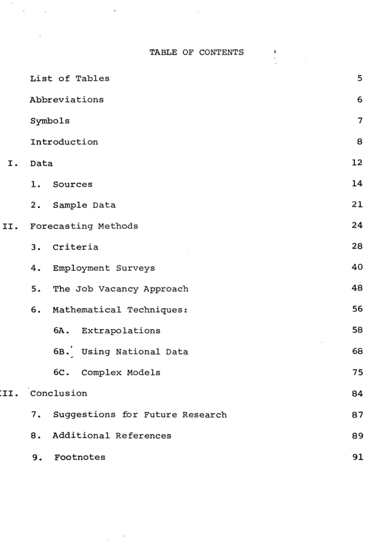
TABLE OF CONTENTS List of Tables 5 Abbreviations 6 Symbols 7 Introduction 8 I. Data 12 1. Sources 14 2. Sample Data 21
II. Forecasting Methods 24
3. Criteria 28
4. Employment Surveys 40
5. The Job Vacancy Approach 48
6. Mathematical Techniques: 56
6A. Extrapolations 58
6B. Using National Data 68
6C. Complex Models 75
III. Conclusion 84
7. Suggestions for Future Research 87
8. Additional References 89
I Sample Data and Sources 23
II The Accuracy of the Sample in Forecasting
its own Future Employment 45
III Comparison of Vacancy Trends, Boston SMSA 54
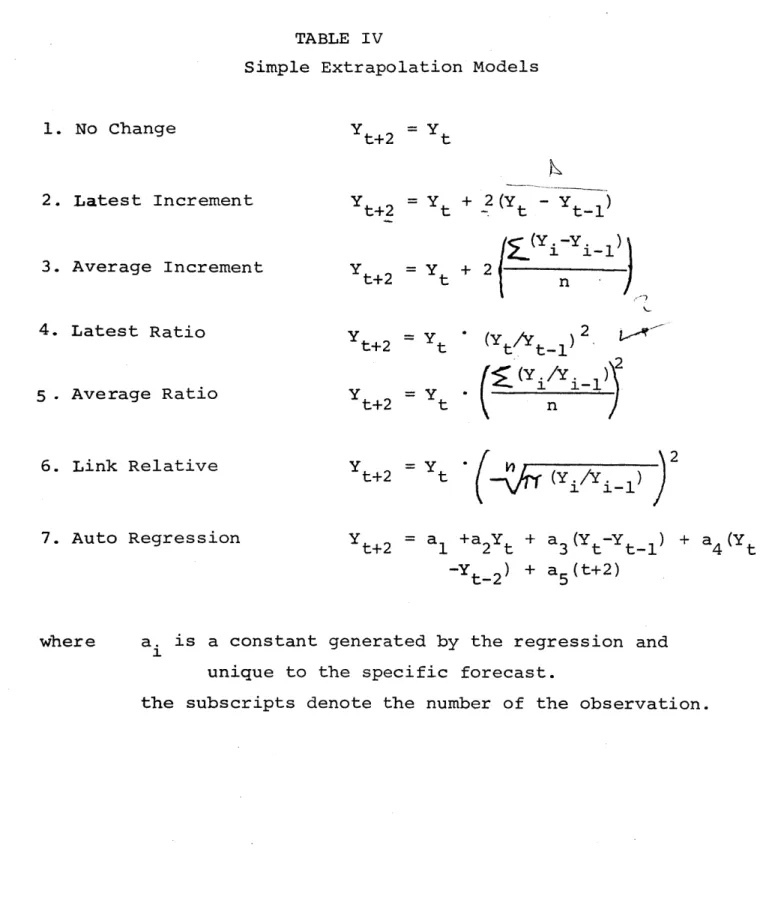
IV Simple Extrapolation Models 59
V Empirical Tests of Various Extrapolation
Methods 64
VI Formulas for Using National Data and
Projections 69
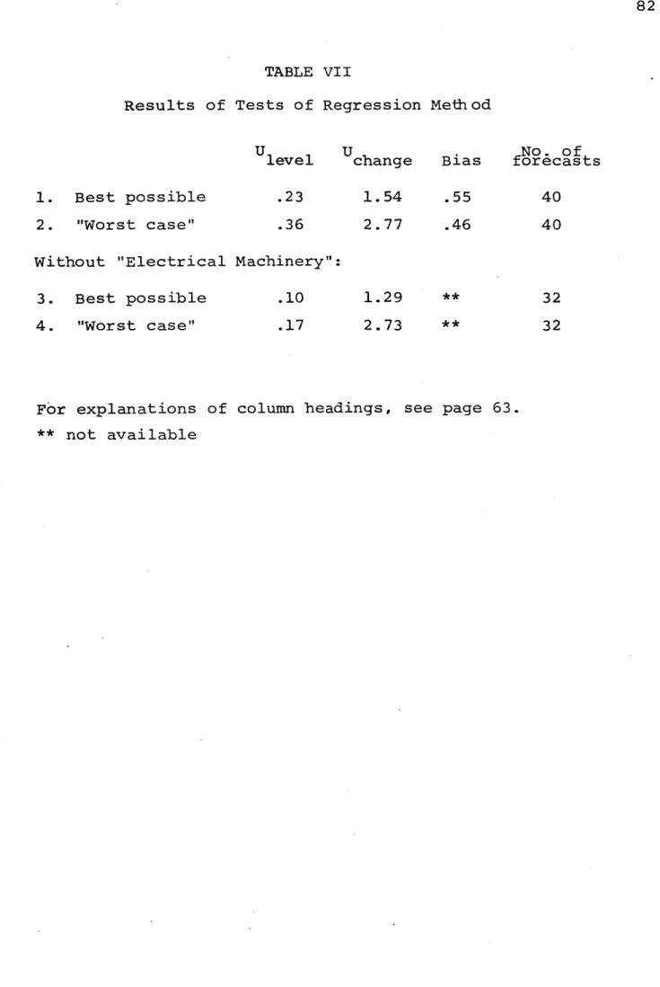
VII Results of Tests of Regression Method 82
VIII Summary of Characteristics of the Various
ABBREVIATIONS
BLS Bureau of Labor Statistics, a section of the U.S. Department of Labor.
DES Division of Employment Security. The branch of many state governments that deals with employment statistics, unemployment security, and job training and placement. If no state name preceeds the abbreviation, the Massachusetts DES, a branch of the state Dept. of Labor and Industries, is implied.
DOT Dictionary of Occupational Titles, Published by the Bureau of Employment Security of the U.S. Dept. of Labor, this defines and enumerates the
standard set of job titles used in most studies. Unfortunately, this system does not completely
agree with the one used by the Census Bureau.
SIC Standard Industrial Classification. Produced by the U.S. Bureau of the Budget, this is similar to the DOT, but lists industry definitions.
SYMBOLS
A random variable, it represents the future (unknown) value of a measurement.
Yt The known value of at time t.
Y f The forecast of at some future time t.
f
e The forecast error, e = Y -
Y
t
t
p(3J) The probability density function of '7 (or, if
V
is discreet, the probability distribution) . It gives the probability that will be any given value. U, The inequality Coefficient, a measure of forecastaccuracy. Lower values of U correspond to greater accuracy. See page 36,
The standard deviation of if . This measures the width of the distribution of . 67% of the area
under p( ) lies within one standard deviation on either side of the mean.
RMS Root Mean Square. A measure that describes the width of a distribution, and a form of averaging. RMS of
E The expected value of , the mean of pf(s). E = Y..- y
if3
7is
discreet, and if ay,is continuous.
Summation of all following terms.
a- Y =
a
Y + aY + aY + a Y 1i
1
2 2
3 3
4
4
Multiplication of all the following terms, similarly to
INTRODUCTION
John Q. Public opens his morning newspaper to discover that unemployment has risen another .1%. Several minutes later he is perplexed to discover page after page of
classified ads begging for people to fill vacant positions. The principal of a local vocational school is dismayed by the number of his well-trained students who can't find jobs, while the president of a nearby company has to turn down
orders because he can't find enough skilled people for a few crucial operations.
These are not uncommon scenes in the U.S. today. For some reason, there is a serious mis-match between the
available jobs and the available people. When the match is correct, there are other barriers to bringing together the
two parts. The result is a tremendous cost to our society in terms of reduced productive capacity, reduced purchasing power, and government support payments.
Ou.t of the concern over this problem the field of Manpower Planning has grown markedly over the last decade. While there has always been some planning, the increasing
mis-match between jobs and workers, plus the rising faith
in systematic research and planning, has prompted considerable expenditure by federal and state governments in the field. The outcome has been a proliferation of forecasts and
statistics, and a pressure to produce even more, that crowds hard on the available techniques. Under such pressure it is not surprising, but especially dangerous, that there has been relatively little research on the planning techniques themselves.
Manpower planning is a broad field, including occupational training and re-training, collection and interpretation of
statistics, and research on educational methods and hiring practices. This paper concentrates on one aspect of it,
the forecasting of future levels of employment. By this I mean the estimation of the future number of jobs of a
specific type, like the number of drill-press operators in Eastern Massachusetts in 1974. 1974 is referred to as
the "target date."
These forecasts may be made by companies to plan their hiring and training programs, by schools to plan their
curricula and to counsel students, by economists to predict changes in the economy, or by governments to plan and fund re-training and placement programs. Obviously, each use will impose different constraints and needs on the
forecasting process. In this paper I will be concerned only with forecasting to plan training, re-training, and placement programs, like the Massachusetts Division of Employment
Security's MDTA program. This fits most state employment-forecasting programs, and some private ones. All remarks in this paper should be taken within this context only.
As the title suggests, this paper critiques and evaluates several common forecasting techniques. For lack of time, no attempt was made to include all known techniques. Rather, those methods most commonly used by groups charged with this type of manpower planning were
included. These are generally simpler (though not
necessarily less accurate) ones. Evaluation of the more complex ones, and the ones just being developed, has been
left to the economists and researchers who are their main users.
As all forecasting requires data, the first section of this paper will deal with that topic. The types and characteristics of data needed are discussed, followed by a quick sketch of the existing sources in the light of
those needs. The sample data used in the empirical testing of the different methods is then introduced.
The section after that discusses the forecasting methods themselves. After a review of the appropriate criteria,
the methods are considered in turn, including the results of the tests. The paper then concludes, as all good papers do, with its conclusions about the utility of the different methods and some suggestions for future research efforts.
Before we begin, a few words of caution are in order. First, there is no one right answer, no "best" method. Decisions about any process, including employment
forecasting, must be made by balancing alternatives in light of the current situation. The appropriate technique will be different for different groups, and even for
the same group at different times. While research like this can help clarify the alternatives, it is not a substitute
for personal judgement.
Second, there is no way to theoretically determine the truth. The best forecasting method is the one that works best. The empirical testing in this paper is of necessity limited to a specific class of employment. 1
There is no guarantee that these results will hold for other data, and any group contemplating a major foray into
employment forecasting is strongly urged to conduct its own tests. The value of this paper, it is hoped, will lie as much in its construction of a framework and method
for evaluating the techniques as it does in the specific recommendations themselves.
DATA
Any forecasting requires information, and the specific type of forecast sets certain criteria for that data. While information never exists that totally satisfies all the
criteria, some data are better than others. In view of the projection techniques to be discussed, the following
charact-eristics seem desirable in employment statistics:
1. Employment must be separated by skill-group within an industry. To prepare proper training programs, etc. the required skills of the available jobs must be known. Currently, the detailed occupational title is taken as a proxy for required skills, but this is not always adequate. It is also useful to know the average or starting wage of an occupation. Wages indicate undesirable, unwanted, or inadequately-paid jobs. The amount of dis-aggregation depends on the
final use of the forecast, but 3-digit DOT 2 titles and 2- or 3- digit SIC codes seem about right for planning training and placement programs. An example of a 3-digit occupation is "Flame and Arc Cutting." A 3-digit industry is "Office Machines."
2. A distinction should be made between different labor markets (towns, SMSA's, states, etc.) depending on
which is the relevant one for that occupation and industry. While a teacher might seek work all over eastern New England, a custodian would generally not
look outside his home city.
guide than the number of employed people, since workers may hold several different jobs.
4. Part-time work must be distinguished from full-time, to avoid training workers for under-employment. The concepts of "part-time" and "under-employment" may have to be re-defined in an era of shrinking work weeks
and increasing numbers of multiple jobholders.
5. Comparability over time is needed to isolate trends and fit models. Comparability between series of data is useful to check and update them. Comparability
between industries permits summing similar skill-groups across industry lines to find total demand.
6. As many observations as possible within the study years are needed to confirm and isolate trends, and
remove random effects.
7. The data should come from periods where conditions external to the data are constant, or their changes can be compensated for. In most cases this limits forecasters to post-WW II data, and in some cases to only the past decade.
8. If the universe of interest cannot be wholly
questioned accurately, the sample must be of sufficient size and composition that sampling error is minimized. 9. While recent data is always nice, it is only of
paramount importance in a few rapidly changing industries. For the rest, the current analytic tools are not
sufficiently keen to warrant it. The allowable time lag generally depends on the frequency of the data
and the length of the forecast.
Several government agencies publish employment data.3 The U.S. Bureau of the Census makes the Census of Population decenially. The 1960 Census reports the employment in 600 occupations by sex, urbanity, and experience for each state, and by sex for SMSA's of over 250,000 people (which is most of them). It also reports employment in 100 occupation groups for 43 industry groups (called the occupational-industry matrix) and wages for 300 occupations for states
and these SMSA's. While this is a very useful disaggregation, it is very difficult to compare on Census with another,
as occupations are merged and separated from year to year, and titles change. Moreover, even if the 1950, '60, and '70 ones were comparable, there would be only 3 data points since World War II. The number of persons holding jobs is used, not the number of jobs held, and part-time work is not
separated. The accuracy varies from Census to Census as the sampling proportion changes, although the latter never drops below 20%.
The Census Bureau also conducts Censuses of Business, Manufactures, Transportation, and Government at 4- to 5-year
intervals, and an annual report on "County Business Patterns." While several of these contain good series on employment by industry and area, there is no occupational breakdown to speak of.
The Department of Labor's Bureau of Labor Statistics (BLS) reports several series. "Employment and Earnings and Monthly Report on the Labor Force" (monthly data for the U.S. as a whole) and the annual "Employment and Earnings Statistics by States" both list employment by industry, not
occupation, to various levels of disaggregation.
The "Job Openings and Labor Turnover" (JOLT) series, published quarterly, is collected in two parts by the Massachusetts Division of Employment Security (DES) for the Bureau. Labor turnover (separations and accessions) has been collected quarterly from a sample of about 2000
firms throughout Massachusetts since 1958. It does not include occupation, skills, or wage, nor is it broken down by market. Current job openings have been collected quarterly
from the 60% of this 2000-firm sample that is in the Boston SMSA since 1969. The series includes occupation, industry, and wage, but its accuracy is limited by the employers
willingness to volunteer information about vacancies. The use of an un-structured questionnaire, permitting
the employer to use non-standard or ill-defined titles, severely reduces comparability. Both sections have very high (85% - 90%) response rates, primarily because
non-respondents are dropped and replaced. This calls into question the randomness of the sample. Problems also arise from the lack of employment data with which to compare
vacancies. Neither series accounts for part-time workers. The Bureau is currently starting a new series, the "Occupational Employment Survey" (OES). This will be
conducted semi-annually by the BLS and state agencies. It is envisioned as a 33% sample of manufacturing firms, followed by a smaller one of non-manufacturing ones. The manufacturing questionnaires were distributed to the 3200 Massachusetts
firms in October of 1971, and results are currently being compiled. The survey includes industry and occupation, but not wages. The survey is such that reporting by labor
market can be done. The use of a structured questionnaire, with titles and definitions keyed to the Dictionary of
Occupational Titles (DOT) will maintain comparability. The use of a staggered sample, in which all the large firms and a portion of the small ones are chosen, will facilitate covering a majority of employees, thus reducing sampling error. As in JOLT, no distinction is made for part-time work. As in all surveys, employees doing two jobs in the
same firm are only counted in their "major" role.
While not a regular series of statistics, the BLS has been constantly conducting Industry Wage Surveys since
1946. Only some industries are surveyed, and those that are are done at irregular intervals of several years. The wages and employment for each occupation are given, and
the use of DOT titles and constant survey techniques maintains comparability. The surveys are for specific geographical
areas that correspond to labor markets, and staggered sampling increases accuracy, but the small number of industries,
areas, and observations severely limits the usefulness of this series on a large basis. There is a similar series of Area Wage Surveys, reporting on major industries in an area. The problems are the same.
The Massachusetts Division of Employment Security (DES) collects figures on unemployment insurance taxes, ES-202, but these do not include wage or occupation, and ignore the large number of workers not covered by the program.
The Division's Job Bank, acting as a referral agency,
solicits listings of job vacancies from employers and publishes a monthly summary. This series suffers from the same problems as JOLT, above, plus the fact that there is no specific
sample, as anyone can call and list a vacancy.
Several series, with varying degrees of usefulness, are published for specific occupations. Most
professional societies, and some unions, publish yearly membership totals by occupation, but these exclude
non-members doing similar work, and include non-practicing non-members which, in fields like nursing, constitute large groups.
The U.S. Office of Education publishes yearly data on
public elementary and secondary school staff, and estimates of similar figures for non-public schools and schools of higher education. While the accuracy is fairly good, 4
and the series involve almost yearly sampling back to the 1920's, changing definitions and levels of aggregation reduce comparability somewhat.
The reasons for the paucity of data are twofold:
First, the accent on re-training programs, and the consequent need for occupational breakdowns, has come only in the past decade. All the older series reflect the previous concern with the "health" of the various industrial sectors of the economy. Therefore, they only contain statistics by
industry.
.Second, in the end data must be gathered by survey, and surveys take a great deal of time and money to prepare and conduct. For example, the BLS's OES survey was first conceived of in 1963, but it wasn't until late in 1971
that the first questionnaires were mailed. The intervening period contained a continual process of definition and
questionnaire development and testing. It takes approximately 2 - 3 man-months to fully develop and test a questionnaire for one industry. 5
There is also a great deal of work andi time involved in getting responses. In the Massachusetts section of the OES survey, conducted by the state Division of Employment
Security, questionnaries were mailed to 3200 firms in October, 1971. After several months duplicate questionnaires were sent to the 2000 firms who had not yet replied. In March, 1972, a third set of questionnaires were sent to the
1500 firms still unheard from. Of the 1700 responses, 300 could not be used, do to business failings, product changes, etc. As replies are still coming in, officials
would not estimate the final response figure, but they did expect it to continue into the summer.
Of the 1700 responses, 25% required telephone calls from either the employer or DES. Just the process of mailing out forms, and soliciting and dcking responses has involved one researcher and two clerks full-time since
the summer of 1971. The long time lags also involve a loss of accuracy. Employers were asked to give data pertaining to the week of 12 May, 1971, for compatability with other surveys4. Any follow-up work done now will be asking for data that is nearly a year old, on a subject where few
written records are kept. Moreover, in a few industries one or more of the major firms hasn't responded, greatly
reducing the sample size, and thus the accuracy.
After the responses are in, additional work remains in the form of coding and editing them, keypunching and punch-validation, writing, testing, and running the data-processing programs, and interpreting and publishing the
results. This entire process, with the exception of the original survey development, will have to be repeated every two years to produce a useable series.
There are three main reasons for employers' reluctance to respond to such surveys. First, they don't wish to
divulge any operating information, for fear their competitors will learn it, in spite of the collecting agency's promise
of strict confidentiality. Second, there is no personal incentive for them to do so, as the final data will be
published regardless of any one firm's decision to participate. Therefore, why go to the trouble? The BLS is attempting to rectify this in the JOLT program. In the future, it will compute each firm's turnover rate, and the industry average, and feed them back to the respective firms, thereby providing
an incentive to respond. Thirdly, few firms keep records along occupational lines. Most maintain a single, uncat-egorized payroll and, especially the larger ones, have
only a rough idea of the number of workers they have in each occupation, as the number is constantly changing. Of those that do keep records, the classifications don't always
coincide with the DOT titles used in most surveys. The situation, though currently poor, is getting better. Because of its occupational structure, use of standard titles, and large sample, the OES survey should, after 6 or 8 years, begin to provide a useful series from which to project. However, there is still room for
improvement. The required skills and current wages of each occupation could be included. Unfortunately, inclusion of
such data now would require a whole new cycle of development and testing, involving costs that might outweigh the
benefits gained. Were the survey being first designed
now, questions to obtain this data could be added at little additional cost. The amount of part-time work could be added now, involving primarily problems of definition, but tools and concepts to handle this information will have
More progress could be made towards inpreasing accuracy and decreasing costs. The Census Bureau system, in which enumerators are sent out April 2 to gather data for April 1, would increase accuracy. Explanatory letters sent several weeks beforehand would encourage participation. A short
reply form with these letters would give advance warning of closed businesses, product changes, and recalcitrant firms, thus avoiding later problems and hastening processing.
All but the first of these involve an increase of accuracy with an increase (sometimes quite small) of cost. In cases where the accuracy is quite sufficient, costs can be reduced
by states "sharing" the survey. For example, Connecticut, Rhode Island, and Massachusetts would each sample one-third of theindustries and pool results, under the assumption that the occupational structure of an industry is the same throughout the region. Absolute figures would come from
state-collected industry employment totals. Such an arrange-ment would decrease operating costs to about 1/3 of previous levels, but if the assumption is true, would reduce
theoretical accuracy by 1/3 (increase standard error by a factor of-i).6 This would be particularly useful in
situations where the uncertainty of the forecasting method far outweighs that of the data.
SAMPLE DATA
A sample set of employment data was gathered for two reasons. First, it was the best way to become familiar with the available data sources and their shortcomings.
These were discussed in the preceding chapter. Second, it was necessary to have data in order to conduct empirical
tests of the methods themselves, as described on page
In view of the importance of making employment forecasts by occupation, as distinct from by industry, I had originally
intended to conduct the empirical tests on occupational employment data. Only one occupation, teaching, had a sufficiently long series of statistics to permit a
meaningful test. Since this would not allow much general-ization, a substitute had to be found.
Therefore, employment by industry data was used. This involves the definite assumption that results from this
type of test are generalizable to occupational forecasting. I have no way of testing whether this assumption is true, but it seems accurate for the precision with which I am
reporting my results. It must be stressed, though, that the reader should not assume any greater precision of the comparative accuracy figures, as this assumption does not support it.
Even within the industry employment statistics we are somewhat restricted. In order to compare methods
accurately, we would like to be able to use the same sample data on all of them. The method with the most stringent
(see chapter GC). This requires at least 10 observations of each of four variables: wages, employment, capital stock, and value of output. The only source of statistics of these
four variables, at any useable level of disaggregation,
was the yearly Massachusetts Census of Manufactures, produced by the Massachusetts Department of Labor and Industries.
Unfortunately, this limits our data to manufacturing employment, but we have no choice.
The other restriction is on the geographic area covered by the data. Ideally, the forecast area should coincide with the labor market area, which is usually
(for urban areas) the Standard Metropolitan Statistical
Area, or SMSA. But the Census of Manufactures has no listings for SMSA's, and only has capital stock figures at the city level. Accordingly, the sample data is for the City of Boston, and covers all factories located within the city
limits.
The time span of the data should be as long as possible to allow the greatest number of trial forecasts. The obvious economic limits were the end of World War II to the present, since the economy was very different outside this span.
However, imperfections and holes in the data series limit the useable span to 1945 through 1969 for employment figures, and 1948 through 1969 for the rest.
The data series used, and their sources, are given in Table I. The industries used are State Census of
Manufactures definitions, which may not coincide with SIC definitions. They are:
Men's and Women's Clothing Printing and Publishing Sausages and processed meats Electrical Machinery Breads and Bakery Products Foundary Products Boots and Shoes, except Rubber
TABLE I
Sample Data and Sources
Series Source
Production Worker Employment Total Depreciated Capital Stock Total Wages of Production Workers Total Value of Output, f.o.b. plant Consumer Price Index, Boston
(Used to deflate W, X, to constant $) GNP Implicit Price Deflator,
Producer's Durable Equipment (Used to deflate K to constant $)
State Census of Manufactures
Is
Is
It
BLS, in Statistical Abstract of the U.S.
U.S. Dept. of Commerce, "Current Business"
All figures in current dollars.
All series yearly, 1948 - 1969, except L, which is yearly 1945 - 1969. Abbrev. L K W X CPI KI
FORECASTING METHODS
Let us now examine some of the more common forecasting
techniques. In this chapter I will give a brief description of the types and methods to be discussed. In the next,
we will consider the different types of forecasts in greater detail, and the criteria by which they are to be
evaluated. The following chapters discuss each method in turn, according to the criteria developed. Where appropriate, the results of empirical tests of the methods will be introduced.
There are several types of forecasts. One is a Point forecast, which predicts that the actual outcome will be a specific value, such as "1000 draftsmen will be
employed next year in Boston." These are the most common, as single numbers are the most familiar and the easiest
to work with. A second type is the Interval forecast, which specifies a range and a probability that the outcome will be somewhere within this range. For example one
might forecast that "There is a 75% probability that employment of draftsmen will be between 800 and 1200 in Boston next year." These forecasts are not common, because users of forecasts dislike working with
probabilities and intervals.
The third type, the Distributional forecast, specifies the "a priori," or expected, probability distribution for
the unknown value. In other words, it describes the probability of each of the possible outcomes, usually by
employment forecasting because it is so unfamiliar, so we shall not discuss it further in this paper.
. IA forecast can also be Conditional. This means that the future outcome is only expected if some intermediate event occurs. For example, "Employment of Engineers
will drop in 1974 if the Viet Nam War has ended by 1973." The user of the forecast must evaluate the probability of this intermediate event himself.
It must be stressed that type, conditionality, and method are merely three non-exclusive descriptors of a
forecast. Any method may be used to make any type of forecast, conditional or not. In the rest of this paper, a distinction between types, conditionality, or methods is only made where it affects the matter under discussion.
All the forecasting techniques discussed in this paper are more or less fixed procedures. But economic theory is not yet developed to the point where fixed procedures can be made as sensitive to the nuances of a particular labor market as the judgement of a knowledgeable
labor economist. Therefore, the results of all of these methods should only be considered preliminary forecasts.
They must be analyzed by someone familiar with the particular labor market to produce the final forecast.
Just as judgement cannot be replaced, it cannot be duplicated in the laboratory. Therefore, none of the
following discussion pertains to this judgemental aspect, but only to the preliminary forecasts. References to the need (or lack of need) for economic knowledge also only
refer to these forecasts. This is done because a forecaster may wish to divide the work so that less skilled staff,
who may lack this knowledge, prepare the preliminary forecast, and senior staff do the final analysis.
One of the most direct forecasting methods is the Employment Survey. A representative sample of employers is queried about their expected employment at the
target date. The result is then inflated proportionally to obtain a forecast for the entire labor market. While it is rarely done, it is possible to survey employment agencies instead, and the procedure is the same.
The Job Vacancy approach uses data on unfilled job openings instead of employment statistics. While any technique could be used to project this data into the
future, some form gf simple extrapolation is generally used. The data can come from employer surveys of current job openings or from listings with employment referral agencies, like the DES's Job Bank.
Extrapolations are simple mathematical formulae that project past data into the future, usually only requiring a few past observations. There are a large number of such
formula'e, of varying complexity. A representative sample will be discussed, including auto-regression, a technique which constructs the formula by fitting it to the actual past data.
The paucity of local data, plus the large time and
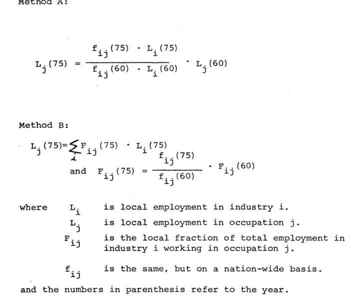
skill costs involved in adding human judgement to mechanical techniques have forced many states to base their projections of the use of National Data. This is not a single technique, but a general approach. In some cases just the past
national matrices of occupational employment by industry are used. In others, the local governments use national
projections prepared by the BLS for this purpose.
If the resources and skills are available, it might be preferable to use a more complex method. The
important distinction here is that the data on the past that goes into the forecast includes information on more than just employment. This allows the forecaster to utilize the information from leading variables and other indicators. For example, if, in the past, capital investment usually
started to drop two quarters before employment did, this variable can be included in the calculations. Then, if
capital has just started to fall off, one can expect that employment will start to drop in two quarters. Here, too, there are many techniques, only a few of which will be discussed. Much attention is given to Regression, as it is a component of the other Complex Methods as well. Multi-equation models and input-output analysis, which
include the interactions between the independent variables also, are covered briefly.
CRITERIA
As in any search, it helps to know, as precisely as possible, what to look for. Accordingly, I will now discuss the criteria by which forecasting methods should be judged.
The criteria fall into three groups: requirements, assumptions, and results of the methods. One of the major requirements is data. Data costs time and money
to gather, often far more than that needed to calculate the forecast itself. The amount and quality of data required depends on the method, and on the precision required of the final forecast. For example, a regression over five
independent variables requires six observations on each to produce any coefficients, and several more to produce
reliable ones. More produce greater accuracy of the forecast. On the other hand, the mechanistic technique of extrapolating
from the most recent change only requires two observations. An Employers' Forecast Survey requires no data, as it
generates its own. In evaluating existing forecasts,
especially ones using previously-collected data, a distinction must be made between the amount and quality of data actually
required by the forecast, and the amount and quality collected by the source, for whatever reason.
All of the methods also require a certain amount of skill and knowledge to execute. While the projection of job vacancies only requires simple arithmetic, the
Employers' Survey requires a knowledge of surveying techniques, and multi-equation models require an extensive knowledge
of economics, econometrics, and electronic data processing. As skilled manpower is usually scarce, this requirement,
too, can cost money.
Another requirement is time. The more complex a method, the longer it takes, generally, to prepare a forecast.
This sets an absolute limit on the frequency of forecasts, and is a large factor in determining costs. Time is
closely related to the amount of work (computation, editing, etc.) involved, but there are slight differences. In
the data collection phase, much time must be spent waiting for survey returns, such time being determined by the
response rate and not by the work load. Work also creates cost in addition to the cost of the time, such as the cost of electronic data processing (EDP).
Different techniques will have different sets of
requirements. Some require more time, some more data, and some more of both. There is no single way to order them for all forecasters. However, all of these requirements can be translated into money costs. If a forecasting group has some idea of what its resources cost, it can
determine the total cost of doing a forecast using each method, and thereby impose some order on the collection. Obviously, different groups will have different cost
structures and a different set of "final costs." It
should be remembered that even already-acquired resources, like existing staff and computers, are scarce, and
therefore have real costs, in that something else would have to be forgone if they were utilized in forecasting.
The rest of the criteria cannot be so easily fit into a cost structure. The first of these is "What assumptions does the forecast make, either explicitly or implicity?"
In some cases the forecaster has to explicitly assume future values of variables. A special case is the Conditional forecast (see page ). In calculating the forecast, he will assume the conditions to hold, but in reporting it he will not, and it is up to the user to determine the probability of the conditions coming true. He also must determine what difference (to the forecast) a change in these conditions would make. A good example of this is the Census Bureau's projections of the U.S. population through 1980.7 It is actually five different projections conditional on five different fertility rates.
In other cases there is only the implicit assumption that the external environment will remain unchanged. Given the current frequency of wars, depressions, etc.
this is a questionable assumption. In any case the
forecast's accuracy will depend on the accuracy of these assumptions. As such accuracy is not known at forecast
time, the assumptions must be judged by their "reasonableness" given the current knowledge. Implicit assumptions are
particularly dangerous, as the forecaster might not realize that he is making them.
The result of the application of a forecasting method to data is a forecast. It may be specified in several ways: Interval forecasts are statements that there is
such-and-such a probability that the actual value Y will turn out to be in a certain range. Rightly or wrongly,
few agencies make such forecasts, since most people prefer to deal in specific numbers. Instead, they make Point
certain number Y1 . But the probability of being
exactly equal to Yi is small, and no forecaster would consider himself "wrong" if he were only off by a few decimal
places, so there is obviously the idea of an interval here too.
One interpretation of point forecasts is that they predict very small intervals, usually specified by the
precision to which they are reported. However, most employ-ment forecasts are reported to single units, and few
forecasters expect to be that correct. Moreover, few would tell you the probability they associate with so small an interval. Or point forecasts can be interpreted as the mean of a predicted probability distribution for Y. But here, too, few forecasters could describe the implicit
distribution, or even its standard deviation. So we must approach the problem from the other direction: We will take the point forecast to be the mean of an unknown distribution, and from examination of the distribution of
error in the past, we will determine the actual
distribution that can be associated with that forecast. 8 If the forecaster is a gypsy, gazing into her crystal ball, then we have no reason to assume that the distribution of errors will remain unchanged. But if the forecast
comes from a standard mechanical process that will not itself change, we can be confident that the pattern of future errors, and hence the probability distribution of a single forecast, is the same as the existing pattern. The narrower this distribution around the forecast point the smaller the expected error, and the better the forecast
method.
Of course, past error distributions and"a priori" probabilities only coincide when an infinite number of observations are made. As that research is beyond the scope of this paper, we will have to content ourselves with a finite, and unfortunately small, sample. This substitution reduces the accuracy of our tests, and must be compensated for by treating the resulting figures as
approximations only.
Having now interpreted the types of forecasts, we must decide what factors we are looking for. A major one is
accuracy: How close does the forecast come to being "correct"? We want to be able to find a single measure of
accuracy for comparison purposes. To do this, we must compare the forecasts, Yf , with the actual values y. It is, of course, impossible to measure the accuracy of a forecast whose target date has not yet occurred.
As we want as many observations on each method as
possible, we must be able to apply the method to different data series and be able to relate the results of the
various series to the single accuracy-of-method term. .Conditional forecasts in which the stated conditions have occurred are judged as regular forecasts. Where the conditions haven't come to pass, no sound judgement can be made. It is not enough to merely substitute the correct initial values and crank through the forecast. In many cases the arrangement of the forecasting method depends on the initial values. Moreover, all forecasts
which cannot be mechanically reproduced and, cranked through.
Similar to conditional forecasts is the problem of policy changes. All forecasts are based on current or
expected policy. If that policy is changed, in response, say, to an unattractive forecast, the future conditions will, hopefully, be changed. While this might affect
the accuracy of the forecast, it should not count against the forecaster. For example, if the forecaster predicts a shortage of draftsmen, and training programs for
draftsmen are accordingly started, they may remove or prevent the scarcity. While the forecast was "wrong,"
it was still very valuable.
Moreover, the labor market responds to forces of supply and demand. The extra draftsmen may reduce the real wages of the occupation, thereby encouraging more firms to seek draftsmen. Thus, there could still be a scarcity, but at this new equilibrium point, which will be different from the forecast. It is very difficult to sort out these effects, and determine how accurate
the forecast would have been in the absence of any policy change, without detailed knowledge of the labor market involved.
For interval forecasts, accuracy is easily measured if the probabilities associated with the intervals are held constant. The fraction of actual values that fell within their predicted intervals, divided by the constant
forecast probability, is a ratio that is independent of the actual data being forecast, and is thus comparable
between trials and between methods.
For point forecasts, the problem is more difficult, as we must reduce an entire distribution to a single term. A measurement of accuracy, U, must meet the following
criteria:
1. It must account for muliplicative and additive scaling. This means that larger absolute errors can be tolerated when forecasting larger quantities. This is a linear relation. Therefore, let us consider
f f
two forecasts Y and Y2 , and two actual values Y f f
and Y2 f 1= kY2 and Y =kY2 then the accuracy of the two forecasts is equal and U =U
f
fl12
. But if Y =k+Y1
2
and Y f= k+Y2 2 k> 0) then Y is a closer fit, and U should be "better" than U 2. These concepts
also apply to two series with different means.
2. U must be independent of the number of terms in the series being inspected.
3. U must be order-insensitive. In producing a single measure of accuracy for a series of predictions and errors, it must be immaterial which predictions are evaluated first.9 Otherwise, identical series, in opposite order from each other (i.e. one ascending and one descending) will generate different U terms. 4. It must be distortion-free. This means that the best guess of a forecast, given the available data, produces the best quality rating. This is an
important, though rarely-investigated, criteria. Consider the forecaster who, after applying his
techniques to his data, has arrived at a probability distribution p§ ). The specific number he will chose as his point prediction should be the expected value
of , E , which is the mean of p( ). It is important that this point have the best expected U-value, EU. To see the effects of a distorting measure, consider
a series of actual events Y and two sets of forecasts, one always at E and the other at EU. Assume further
that the forecaster was correct, in his choice of p MO). Over a long series, the mean of Ywill be E
and this will have the smallest average error, but
the forecast at EU will have the best overall U-rating. Thus the rating system will give a distorted view of
the forecast value. This may seem obvious, but as popular a measure as the absolute percentage error
seriously violates this criteria. 10
Having established our criteria, let us consider briefly several common measures of forecast accuracy. Throughout the discussion, let "e" stand for the error
f
between forecast and actual value,Y. - Y.. A popular l1
measure is the standard deviation of the errors, - = It is distortion-free, but does not handle multiplicative or addative scaling. As such, it is a good measure for comparing different methods applied to the same single series. The Mean Absolute Percentage
and RMS Absolute Percentage I 7- are not
distortion free, as is not the original version of Theil's
Inequality Coefficient 1
l
. The correlationbetween Y. and Y., and the ratio of variances O7T
1 1
lT for a neie wit the sae varia nr, rTgarrd le C7~_
of the actual errors involved. C does not scale. No measure was found that fitted all the criteria
perfectly. The closest one was the adjusted standard 12
error, 4 It meets all the criteria, with the
following exceptions:
1. It is not totally distortion-free, although it is far more so than absolute percentage. In the termin-ology of footnote 10, if =Y thenLE Y is less
than if I/ =Y 2, so U1> U2. But the difference falls off very quickly after the first few forecasts are made, so EUGP E 7.
2. While scaling between series is handled, scaling between terms within a series is not. Thus, errors on values above EY count for as much as the same size errors on smaller Y.. This was considered bearable here because all but two of the series are grouped tightly around the mean, and because no other measure could correct this without introducing a more serious problem itself.
The adjusted standard error, also known as the
inequality coefficient, has the advantage of including the popular economic concept of "quadratic loss." This concept
says that large errors are so bad they are more than proportionally worse than small errors. For example,
an error of four is not twice as bad as one of two, but four times as bad. Quadratic loss considers "badness" as a function of the square of the error =
A second aspect of accuracy is bias, that is the
f
difference between EY and EY Ideally, the forecasts should be evenly grouped around the actual values, so that the mean error is zero. But if the forecasts are consistently or predominantly too low or too high, then the distribution of errors will be "lopsided." Then EY / EY and Ee
#
0. In such a case the point forecasts should be interpreted as only the forecaster's incorrect estimate of the mean of p(y). In interval forecasting such an error will show up as a reduced percentage of "correct"forecasts, not as a specific bias, but the compensation for it is the same. Note that, while the forecasts are still "wrong," this is a very different problem from that of the forecasts being too widely distributed around the
actual values. It is also more easily solved. If all f
forecasts Y. are corrected by a series correction
factor, the entire distribution of forecasts is shifted,
f'.
and a new series of forecasts Y. is generated. The
forecasts are now more accurate, and a new set of standard errors and U-terms are generated. If such a correction is applied to future forecasts, they will be improved, too. Obviously, the correction factor will be different for different series. The factor can be additive,
f'
f f f' f fY. = Y. + (EY - EY ), or multiplicative, Y. = Y.* (EY/EY ),
1 1 1 1
or both. If both terms are desired, they are best
f
determined by a regression of Y on Y. However, in most cases the bias will be very small, and can be ignored.
To find the bias, merely add up all of the errors, including their signs, and divide by the number of errors.
(Bias =2,8-' ). To compare different series, divide the bias by the standard deviation. If the bias is only a small fraction ofC , the forecast can be considered unbiased.
In determining accuracy, the question remains as to which series to measure. While the level of employment
is what is usually reported in a forecast, it is generally the change in employment that is of interest to planners. Moreover, the amount of change from year to year varies
far more than the actual level. Therefore, it is the projected change that should be tested for accuracy. In this paper I have used the methods to forecast both variables, where possible, and have tested both forecasts.
The third aspect of the resulting forecast is its precision. This is very different from accuracy, and refers to the specificity of the projection. It is quite possible to have a very precise forecast that turns out to be highly inaccurate. Conversely, the less precise the forecast, generally, the greater the chance that it
13
will be' correct, but the less useful it will be. None of these methods have any specific inherrent precisions. They all will produce numbers down to the units digit. But the useable precision is limited by the precision and accuracy of the input data, and the effective accuracy of the method itself. Any greater precision reported only creates a false sense of security. Bearing in mind the trade-off between precision and accuracy, it is generally best to report the lowest acceptable precision for the use to which the forecast is being put.
Obviously, accuracy, bias, precision, and assumptions cannot be easily translated into money terms. This would require a knowledge of the effects of manpower policy that we currently lack. However, bias can be compensated for,
and precision, accuracy, and assumptions are inter-related. Therefore, the best way of deciding which forecasting method to use is often to assume fixed resources, and choose the one with the greatest accuracy, or to target a given
precision and accuracy, and choose the one with the least cost. Beyond this, a subjective balancing of costs and results is required that is beyond the scope of this paper.
There is one more aspect of forecasting that is far too often forgotten. Throughout the forecasting process the questions must be repeatedly raised: "Does this
forecast tell us what we want to know?" and, if so, "Will it help to solve the problem at hand?". If the
answer to either question is "No", then the best forecast in the world is a waste of time and resources, at best, and a negative policy aid at worst.
SURVEYS
One method of estimating future employment is to ask employers whom they plan to hire. This can be part of a survey of current employment, or a separate project.
In either case the technique is the same: a representative sample of employers is generated, a target date in the
future is selected, and the employers are asked to estimate their employment at that date, by occupation, including new job categories. The sample totals are then inflated to the universe by multiplying each sub-total by its appropriate scaling ratio. For example, if the sample
of firms currently employing 25 to 100 employees is estimated to include one-fifth of the total employment in industries of this size, the expected employment for each occupation in the zgxup is muliplied by 5. The result is the
estimated employment, by occupation, for all films of that size. Due to their importance, large firms (over 50 or 100 employees) are usually sampled 100%. This is efficient, covering the greatest number of workers with the fewest questionnaires.
The requirements of this method are different from those of other techniques. In the first place, there are almost no data requirements, as the method generates its own data. It is more efficient, in terms of questionnaire size, to have an approximate idea of the occupations that will have large surplusses or shortages of workers. This data, though, can be easily and informally gathered from employment agencies, etc.
Surveying does require certain skills, particularly the ability to construct a questionnaire that is unambiguous and easy to complete. This will encourage responses from busy employers. Also, since a survey of any
reasonable-sized labor market will generate several hundred or even several thousand questionnaires with 20 to 100 items each, it is rather impractical to tabulate the results manually. Therefore, keypunching and programming skills are needed. However, since no knowledge of the labor market is
necessary for this task, it can be sub-contracted out. For example, in the OES survey (see page IS), the
Mass. DES is interpreting the responses, but the BLS is tabulating them by computer.
Time is probably the stiffest requirement. It takes months, sometimes years, to develop a comprehensive,
unambiguous questionnaire. This involves designing one, testing it on a small sample of employers, evaluating
the response, and re-designing it. It also takes a long time, often half a year, between the first distribution of the questionnaires and the returns of the stragglers. While some of this time can be utilized in processing the
early returns, much of it is spent answering respondents questions and waiting. The interpretation and tabulation
of the returns, even by computer, can also take many weeks, since the results must be keypunched and verified before the computer can read them.
In addition, there are several miscellaneous costs which, for a large survey, are not insignificant. There is the printing and mailing of up to several thousand
questionnaires, and the writing and distribution of many follow-up letters to non-respondents. Moreover, there is a considerable amount of staff time involved in answering employers' questions and tracking down non-respondents.
Very few specific assumptions are made by this
method. The only important one is that the sample accurately reflects the entire labor market. While there is no way
of testing this assumption, without constructing an entire second survey, this can be minimized by using as
large a sample as possible. However, the individual respondents do make all sorts of implicit assumptions. They assume the future state of the economy and their market, they generally assume that the labor force will not change, etc. The worst part about this is that first, many employers are not sufficiently knowledgeable about
the economy to make reasonable assumptions, and second, that the assumptions are not reported. Being unknown, they cannot be evaluated or corrected for, thereby intro-ducing an unknown error into the forecast.
The problems are the same as those involved in
"current employment" surveys (see page 1i ) . Furthermore, many employers are unable to project their employment, or are unwilling to divulge the information, so there are fewer responses. There is a greater chance of new
jobs, not in the DOT, being created and listed, thereby increasing processing time and reducing comparability.
It is difficult to test the employment survey
empirically. The conduction of even one such survey is beyond the scope of this paper, not to mention the
number necessary to be able to generalize. The lack of real data by occupation also makes it very difficult
to test past surveys. However, some idea of the potential accuracy of surveys can be gotten from a Rutgers University
study of the Newark Occupational Training Needs Study. This was an employers survey conducted by the New Jersey DES in Newark in 1963.14
The 1963 survey asked employers to forecast their September, 1965 and 1968 employment. In October, 1965, the Rutgers group distributed questionnaires to 604 of
the 811 employers who had responded to the original survey. These questionnaires listed the employers' forecasts from
the 1963 survey and asked them to list their actual September, 1965 employment and to attempt to explain any differences
from the forecast.
Before we discuss the results of this study, a note of caution is in order. First, since not all of the
employers responded to the follow-up survey, only 77% of the employees covered by the 1963 survey were involved in the te-survey. Thus, it is not certain how much the 1965 results are representative of the actual value of the original survey.
Second, we are still only discussing a single employ-ment forecasting survey. There are many aspects of the 1963 survey, such as sample size and type, nature of the questionnaire, etc, that may have affected its accuracy. Having no way to control for these factors we have no way to generalize the results of this study to other employment surveys. We can only get a general idea of the usefulness of such surveys.
There are two aspects of survey accuraey to test: How representative of the entire labor market was the
sample, and how accurate was the survey in predicting the future employment of the sample? To answer the first one, Rutgers compared the actual percentage increase in employment of the sample with the percentage increase in employment of the entire labor market, on an industry-by-industry basis. The results were fair. The best corr-elation was in Manufacturing, where a 2.8% increase in the sample almost matched a 3.5% increase in the market as a whole. The worst was in Retail Trade, where the
sample suffered a 2.9% decline while the market as a whole rose 6.5%.
To a large extent, errors of this type were due to small sample size, permitting the characteristics of a single firm to bias the sample, and thence the
projection. Retail Trade was only sampled 6.8% while Manufacturing was sampled 17.8%. This must not be the
only reason, however, since the third worst industry was sampled 41%.
As a general rating of sample representativeness, we can use the inequality coefficient described on page This says, in effect, "Even if the survey had predicted the change in the sample perfectly, how good would the
forecast of the market as a whole have been?" As such, it is comparable with the results of empirical tests of other methods. The inequality coefficient was .94, which is fairly good for forecasting changes in employment.
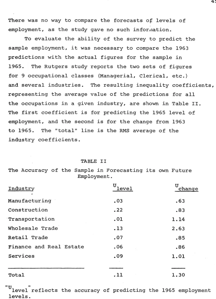
There was no way to compare the forecasts of levels of employment, as the study gave no such infor~nation.
To evaluate the ability of the survey to predict the sample employment, it was necessary to compare the 1963 predictions with the actual figures for the sample in 1965. The Rutgers study reports the two sets of figures for 9 occupational classes (Managerial, Clerical, etc.)
and several industries. The resulting inequality coefficients, representing the average value of the predictions for all
the occupations in a given industry, are shown in Table II. The first coefficient is for predicting the 1965 level of employment, and the second is for the change from 1963 to 1965. The "total" line is the RMS average of the industry coefficients.
TABLE II
The Accuracy of the Sample in Forecasting its own Future Employment.
Industry Ulevel Uchange
Manufacturing .03 .63
Construction .22 .83
Transportation .01 1.14
Wholesale Trade .13 2.63
Retail Trade .07 .85
Finance and Real Estate .06 .86
Services .09 1.01
Total .11 1.30
"U
level reflects the accuracy of predicting the 1965 employment levels.
"tU
change reflects'the accuracy of predicting the 1963-1965 absolute change.