HAL Id: hal-01724199
https://hal.archives-ouvertes.fr/hal-01724199
Submitted on 6 Mar 2018
HAL is a multi-disciplinary open access
archive for the deposit and dissemination of
sci-entific research documents, whether they are
pub-lished or not. The documents may come from
teaching and research institutions in France or
abroad, or from public or private research centers.
L’archive ouverte pluridisciplinaire HAL, est
destinée au dépôt et à la diffusion de documents
scientifiques de niveau recherche, publiés ou non,
émanant des établissements d’enseignement et de
recherche français ou étrangers, des laboratoires
publics ou privés.
Online Relation Alignment for Linked Datasets
Maria Koutraki, Nicoleta Preda, Dan Vodislav
To cite this version:
Maria Koutraki, Nicoleta Preda, Dan Vodislav. Online Relation Alignment for Linked Datasets. The
Semantic Web, ESWC 2017, May 2017, Portoroz, Slovenia. �hal-01724199�
Online Relation Alignment for Linked Datasets
Maria Koutraki1,2, Nicoleta Preda3, and Dan Vodislav4
1FIZ Karlsruhe – Leibniz Institute for Information Infrastructure 2
Institute AIFB, Karlsruhe Institute of Technology (KIT), Germany 3
University of Versailles, France 4
ETIS CNRS, University of Cergy-Pontoise, France [email protected], [email protected],
Abstract The large number of linked datasets in the Web, and their diversity in terms of schema representation has led to a fragmented dataset landscape. Query-ing and addressQuery-ing information needs that span across disparate datasets requires the alignment of such schemas. Majority of schema and ontology alignment ap-proaches focus exclusively on class alignment. Yet, relation alignment has not been fully addressed, and existing approaches fall short on addressing the dy-namics of datasets and their size.
In this work, we address the problem of relation alignment across disparate linked datasets. Our approach focuses on two main aspects. First, online relation align-ment, where we do not require full access, and sample instead for a minimal sub-set of the data. Thus, we address the main limitation of existing work on dealing with the large scale of linked datasets, and in cases where the datasets provide only query access. Second, we learn supervised machine learning models for which we employ various features or matchers that account for the diversity of linked datasets at the instance level. We perform an experimental evaluation on real-world linked datasets, DBpedia, YAGO, and Freebase. The results show su-perior performance against state-of-the-art approaches in schema matching, with an average relation alignment accuracy of 84%. In addition, we show that relation alignment can be performed efficiently at scale.
1
Introduction
In the recent years, the number of datasets exposed as linked data has grown continu-ously. Estimates show that there are more than 1000 datasets, with roughly 30 billion facts in the form of triples [1]. The decentralized nature of these datasets and further-more, the lack of mechanisms and proper documentation for reusing existing schemas has led to a large number of schemas, 650 in LOD [23]. In many cases classes and relations across such schemas are redundant and not aligned (with only 2% of schemas aligned [23]). As a consequence this leads to a disintegrated dataset landscape [8].
This particular problem has been partly addressed by ontology alignment ap-proaches, which almost exclusively have focused on class alignment across disparate ontologies [25]. In contrast to the class alignment, relation alignment has not seen such progress. However, it is an equally important task, helping address information needs that span across datasets. In this way, through class and relation alignment we can rewrite and perform federated queries across disparate datasets.
The few existing relation alignment approaches, like the state of the art [26] fail to incorporate two main aspects of linked datasets. First, the scale of datasets, by requiring full access on the dataset snapshots. As shown in [23] full access is not always possi-ble, where many datasets limit to only query access and to a few thousands of triples per query. Second, the evolving nature of datasets since the alignments are performed on snapshots. Therefore, on data updates the alignments might not hold, hence, they need to be recomputed from scratch. However, computing such alignments on dataset snapshots will eventually lead to re-computation even for those relations where the cor-responding data has not changed, thus making such approaches inefficient.
We propose SORAL – Supervised Ontology Relation ALignment, a supervised ma-chine learning approach for relation alignment across disparate schemas and datasets. Similar to [16] we work under the assumption that owl:sameAs statements exist be-tween entities across datasets [23]. Additionally we operate in an online setting requir-ing only SPARQL query access to datasets, thus allowrequir-ing for large scale alignment, independent of dataset size.
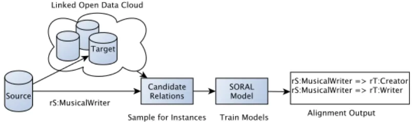
Figure 1 shows SORAL, consisting of two main steps. First, for a source relation and source dataset, we generate candidate relations for alignment to a target dataset. As candidates we consider relations that have entity instances in common (based on owl:sameAsstatements). In this step we employ sampling strategies to cope with the scale of datasets and ensure the efficiency of SORAL. Second, for a relation pair, we compute features from the common entity instances, and information we extract from the relations, e.g. domain/range of relations etc. SORAL optimizes for efficiency by performing the alignment in an online setting, and accuracy by providing qualitative relation alignments. To this end, we make the following contributions:
– We propose an approach for finding relation subsumptions and equivalences; – We perform the relation alignment in an online setting that ensures efficiency; – We conducted an extended experimental evaluation using real-world knowledge
bases (KBs).
Figure 1: SORAL approach overview.
2
Related Work
Scope. Our goal is to discover subsumption and equivalence relationships between the relations of two KBs exported using SPARQL endpoints. This problem is also known as ontology alignment. Ontology alignment includes: instance alignment, class align-ment, and relation alignment. To align relations, we rely on existing work on aligning instances [5,18,6]. Hence, we see this effort as complementary to ours.
Related work in this field is usually categorized in schema-based and instance-basedapproaches depending on the data that is used to produce the alignments. The majority of the work focuses on class alignment and much less on relation alignment, which is the objective of this work.
Schema-Based. Schema matching systems like in [20,3,7,24] align classes by relying on schema constrains, which are often unavailable in LOD. COMA++ [3] expects as input OWL descriptions and ignores data instances. While in [7] the approach relies on user assistance for the alignment process. Other systems like in [24] serve as proxy over existing schema matching tools, thereby providing means on combining the ferent functionalities of the individual platforms. BLOOMS [14], aligns classes in dif-ferent KBs where the schema definitions are available. In our vision, the alignment of KBs should happen even in cases where explicit schema information or other database constraints are not available. For that reason we choose an instance-based approach. Instance-Based: Class Alignment. Many instance-based approaches are proposed for class alignment in ontologies [15,11,29], contrary to our work, that focuses on relation alignment. Movshovitz-Attias et al. [21] infer subconcept and superconcept hierarchies from a KB. [22] produces equivalence and subsumption relationships between classes. Contrary to the class alignment work, the difference in the case of relations lies on two main aspects. First, classes and relations represent two different constructs in schemas. For classes it is sufficient to simply measure set overlap in terms of entities and other schematic information. In the case of relations we have the domain and range which should map between two relations, and even in cases they match, two distinct relations might have different semantics (e.g. bornIn and presidentOf).
Instance-Based: Relation Alignment. A large corpus of works focus on the discovery of equivalence or similarity relationships between relations, with early examples in relational databases [10,19], and Web services [17]. In the case of KBs, the schemas are in large numbers and vary heavily. For example, YAGO and DBpedia vary greatly in their representation, where YAGO has 37 object relations, while DBpedia has 688, whereas in terms of entity instances they have a high overlap. Thus, by considering only equivalencealignments we cannot map relations that have similar semantics or subsume another. This is due to the fact that many relations map to more than one relation in a target KB (e.g. YAGO to DBpedia). In itself finding subsumption relationships is more challenging, yet, it reflects the true nature of this problem. In the following we describe only the approaches that are capable of handling subsumption relationships [28,26,30]. ILIADS [28] and PARIS [26] serve for the dual purpose of aligning instances and schema elements between two KBs. In ILIADS the authors acknowledge the difficulty of the relation alignment problem, where systems designed for class and instance align-ment perform poorly. In the case of PARIS, it is acknowledged as a state of the art approach by related work [30], thus, we compare against it, and show the advantages of SORAL achieving significant improvement over PARIS. Gal´arraga et al. [12] pro-pose ROSA, a relation alignment approach. ROSA operates on a similar setting as ours. However, as we show in our experimental evaluation in Section 7, relying solely on association rule miningmeasure PCA [13] is insufficient. Finally, the aforementioned works [28,26,30,12] operate on KB snapshots, contrary to our approach, which operates
on small data samples that are queried from the respective KBs, thus, tackling one of the major problems of efficiency of existing work.
3
Preliminaries
Knowledge Bases. We assume that knowledge bases (KB) are represented in RDFS1.
A KB consists of a set of triples K ⊆ E × R × (E ∪ L), where E is a set of resources that we refer as entities, L a set of literals, and R a set of relations. An entity is identified by a URI and represents a real-world object or an abstract concept. A relation (or property) is a binary predicate. A literal is a string, date or number.
Given a triple (x, r, y) (aka a statement), x is known as subject, r as relation, and y as object. Based on the nature of the objects, we classify relations in two categories: (i) entity-entityrelations with x and y being entities, and (ii) entity-literal relations where y is a literal.
We use r(x, y) to refer to the triple (x, r, y), and the tuple (x, y) as an instantiation of r. Without loss of generality, for an entity-entity relation r ∈ R we denote its inverse as r− ∈ R, and that the triples of r− are also contained by K (∀r(x, y) ∈ K ⇒
r−(y, x) ∈ K).
Classes and Instances. A class is an entity that represents a set of objects, e.g., the class of all politicians. An entity that is a member of a class is called an instance of that class. The rdf:type relation connects an instance to a class. For example, Barack Obama is a member of the class of politicians: rdf:type(Barack Obama, Politician). Equivalence of Instances. Equivalence between two entities is expressed through owl:sameAs statements. For example, yago:US and dbpedia:USA (both refer-ring to the same country), the equivalence of the two instances is expressed as owl:sameAs(yago:US, dbpedia:USA).
4
Problem Statement
We consider a KB pair (a source KS and a target KT) that can be queried through
SPARQL endpoints. Next, we assume that owl:sameAs statements exist between entity instances of KS and KT. For two equivalent instances es ≡ et, from KS and
KT, respectively, we assume that, KS stores owl:sameAs(es, et) and KT stores
owl:sameAs(et, es).
Definition 1 (Relation Subsumption). For two relations rSandrT, we say thatrS is
subsumed by rT, or thatrT subsumes rSand writerS ⊆ rT orrS⇒ rT iff
∀x, y, rS(x, y) is true → rT(x, y) is also true.
The notion of subsumption is independent of the relation extensions/name in the two KBs. We can only rely on the facts stored in the KBs to learn the subsumption relationships.
Goal. For two knowledge bases, a source KS(ES, RS, ES ∪ LS) and a target
KT(ET, RT, ET ∪ LT), and a relation rS ∈ RS, find the relations rT ∈ RT s.t.
rS ⊆ rT.
The relationship of equivalence between two relations is expressed as two way sub-sumption relationship: rS ≡ rT iff rS ⊆ rT and rT ⊆ rS. In this way, we support the
computation of both subsumption and equivalence relationships.
In this work, we consider only entity relations. We do not consider entity-literal relations, because the equivalences between entity-literals are managed differently and are not materialized in KBs. However, once such equivalences are established, one can use our approach to align entity-literal relations.
5
SORAL: Relation Alignment
We propose SORAL, an online relation alignment approach, which for a pair of knowl-edge bases, a source KS and a target KT, works under two assumptions: (i) each KB is
accessible through a SPARQL endpoint, (ii) for a KB pair we assume that their entity instances are partially aligned.
The process of discovering subsumption and equivalence relation alignments in SO-RALis outlined in two main steps:
(1) Candidates Generation. For a relation rS ∈ RS, find all overlapping relations
rT ∈ RT i.e.∃x, y : rS(x, y) ∈ KS∧ rT(x, y) ∈ KT.
(2) Supervised Model. For every candidate pair hrS, rTi, we classify it as correct or
incorrect depending if the subsumption relationship holds or not. We propose a set of features (Section 5.3) which we use to learn a supervised machine learning model.
5.1 Candidate Generation
We observe that for a relation rSits super-relations rT must have at least one
instantia-tion in common. Thus, they must satisfy the following constraint:
∃xS, yS, xT, yT :rS(xS, yS) ∧ xT ≡ xS∧ yT ≡ yS∧ rT(xT, yT)
Since, the relations reside at different endpoints, for the candidate generation we per-form a federated query. The conjunction of the first three terms of the expression can be evaluated at KS. However, for the last term the query is evaluated at KT. More
precisely, we first evaluate the following query at KS:
Q1: SELECT DISTINCT ?xT ?yT FROM <KS> WHERE
{ ?xS rS ?yS. ?xS owl:sameAs ?xT. ?yS owl:sameAs ?yT. }
From the query result-set SrS = {(x1, y1) . . .} of Q1 we discover the candidate
relationsfrom KT for which these pairs are instantiations. Note that a tuple (xT,yT)
can be the instantiation of the inverse of a relation at KT. Hence, we discover both direct
and inverse relations. For this purpose, we use the VALUES feature from SPARQL 1.1 and compute using only one query both inverse and direct relations.
Q2: SELECT DISTINCT ?rT ?d FROM <KT> WHERE {
VALUES (?x ?y) {(x1 y1) . . .}
{ SELECT ?x ?rT ?y ?d WHERE {?x ?rT ?y. VALUES ?d {"d"}}}
UNION
{ SELECT ?x ?rT ?y ?d WHERE {?y ?rT ?x. VALUES ?d {"i"}}} }
The result-set of query Q2, C(rS), denotes the set of candidate relations rT. For
simplicity, we assume that all relations are direct. This is because we have assumed (Section 3) that each KB defines for each relation, its inverse.
We avoid the transfer of the entire instantiations of a relation (as it introduces a bottleneck), and instead sample for a minimal set of tuples (xT, yT) that are transferred
from the source to the target. We propose sampling strategies and discuss them in the following.
5.2 Sampling Strategies
In many cases SPARQL endpoints place limitations on the number of triples one can transfer. Furthermore, even when full access is provided, transferring the full data is expensive (both in terms of time and network bandwidth consumption).
To overcome these issues we suggest three sampling strategies for entity instance selection, which we use to generate relation candidates. For rS, the objective is to
sample for a minimal set of representative instantiations SrS, such that they provide
optimal coverage on discovering super-relations rT.
First–N Sampling. It is an efficient way to query for the first N returned entity samples (xT, yT). The drawback is that it does not provide representative samples, due to the
fact that it is subject to how the data is added into the KBs. This represents a baseline to show the impact of sampling strategies on generating accurate relation alignments. Random Sampling. In this case we use theRAND()feature of SPARQL 1.1 to query for representative samples for SrS. Contrary to first–N , ordering the matching triples
through theRAND()function is expensive and introduces a significantly higher over-head in the query-execution when performing the relation alignment. Moreover, depen-dent on the sample size, the samples might be biased towards the classes with more instances, and as such it has an impact in the candidate relations we generate from KT.
Stratified Sampling. Here, we account for the possibly missing candidate relations from KT due to the sample size, for relations whose domain/range belongs to fine
grained entity types. Through stratified sampling we can achieve a better coverage in terms of uncovered relation alignments for rS.
We group entities into homogeneous groups/strata (a group is represented by an en-tity type) before sampling. Additionally, the groups are further defined at various depths at the type taxonomy levels in order to find out the optimal groups which yield the high-est coverage in terms of candidate relations. To ensure the disjointness (a prerequisite for stratified sampling), from the transitive type closure for an entity, we associate it to its most specialized type (dependent at what level in the type taxonomy we are inter-ested to group entities), thus, ensuring disjointness of groups.
At high levels in the taxonomy, the sampling is similar to random sampling, whereas for deeper levels, we have more groups, and as a consequence more representative sam-ples, leading to an increased coverage of candidate relations from KT. The query to
retrieve the samples is shown below, where N is the sample size for each strata, propor-tional to the number of entities in it and the given total sample size.
Q3: SELECT DISTINCT ?xT ?yT WHERE {
?xS rS ?yS. ?xS owl:sameAs ?xT.
?yS owl:sameAs ?yT. ?xS rdf:type ?type.
} ORDER BY RAND() LIMIT N
5.3 Features
In this section, we describe the features we use to learn the supervised models in SORAL to predict whether the subsumption relationship for a relation pair holds. We consider features which we categorize into two main categories. Firstly, we consider inductive logic programming (ILP) approaches that work under the open and closed world as-sumptions w.r.t the instantiations of relations rS and rT. In the second group (GRS),
we look into general statistics extracted from relations, specifically we assess the do-main/range class distribution of the relations rS and rT. It is important to note that
the features are computed over the sampled entity instances SrS and for the candidate
relation in C(rS).
ILP – Features Closed World Assumption – CWA. Proposed in [9], cwa is used to mine association rules and was first used for relation alignment between two KBs in state of the art [26]. It works under the closed world assumption, where the KBs are assumed to be complete, hence there are no missing statements. The cwa score is com-puted as in Equation 1. It measures the overlap in terms of the number of instantiations in common between rSand rT, normalised by the number of instantiations of rS.
cwa(rS⇒ rT) := overlap(rS∧ rT)
rS (1)
We gather such counts by querying the respective SPARQL endpoints of KSand KT.
The cwa measure provides strong signal for the alignment of relations in the case when the relations are complete (i.e., KBs have all statements for a given relation). However, due to the fact that KBs are constructed from different sources, complemen-tary statements for an entity in different KBs are considered as counter-examples. Partial Completeness Assumption – PCA. The second feature, pca, is an ILP measure proposed in [13] with the purpose of mining Horn rules for an input KB. It is able to handle incompleteness in KBs, and works under the partial completeness assumption. For a relation rS and instance x, it is assumed that the KB contains either all or none
of the rS-triples with x as a subject. As counter-examples for the alignment rS ⇒ rT,
is considered any pair (x, y) that is an instantiation of rSbut not of rT. More formally,
counter(rS ⇒ rT) := #(x, y) : rS(x, y) ∧ ∃y2, y26= y : rT(x, y2) ∧ ¬rT(x, y).
pca(rS⇒ rT) := overlap(rS∧ rT)
overlap(rS∧ rT) + counter(rS⇒ rT) (2)
Similar to cwa, to compute pca we extract the counts for rS and rT through SPARQL
queries on KS and KT. Note that, pca can have maximal score even when the overlap
helpful in detecting alignments with a small overlap in the two KBs. On the other hand, it increases the likelihood of getting false positives. These are caused by erroneous facts and incomplete data.
However, considering jointly cwa and pca features has the effect of regularizing each other; for high pca scores but low cwa the chance of having a correct alignment is low, and vice-versa. We make use of this assumption and compute a joint probability score for a relation pair being correct by considering the pca and cwa scores jointly. Partial Incompleteness Assumption – PIA. The pca may hold for functional relations (see Equation 4), but is less probable for one-to-many relations. The intuition is that if the average number of rS-triples per subject is high, then it is more likely that not all
rS-triples of some subject x have been extracted. The same observation holds also for
the triples of rT. Note, that we have yet to prove that rS is subsumed in rT. Hence, the
examples of less functional relations should be weighted less than the counter-examples of more functional relations. We measure the pia score as:
pia(rS⇒ rT) := overlap(rS∧ rT)
overlap(rS∧ rT) + (counter(rS⇒ rT) ∗ func(rS)) (3)
where, f unc(rS) measures the probability that a counter example may not exist.
General Relation Statistics (GRS) – Features. In the GRS feature group, we pro-pose features that take into account the cardinality of the two relations, and the types extracted from the entity instances in the domains and ranges of a relation.
Functionality of a Relation. A relation is called functional, if there are no two distinct facts that share the relation and the first argument. Real life KBs may be noisy, and contain distinct facts for relations that should be functional (such as bornIn). Therefore, we make use of the functionality [26]:
f unc(r) := #x : ∃y : r(x, y)
#(x, y) : r(x, y) (4)
Perfect functional relations have a functionality of 1.
From this intuition we assume that if rSis subsumed by rT, then the number of facts
per subject in rS should be lower than in rT. In other words, the functionality of rS
should be grater or equal to the functionality of rT, that is if rS ⇒ rT → f unc(rS) >
f unc(rT). Finally, the functionality feature we consider here is the functionality
differ-ence between rSand rT, f uncdif f := f unc(rS) − f unc(rT) ∈ (−1, 1).
Weighted Jaccard Similarity. We measure the similarity of the type distributions D(·) between the relations rS and rT. We denote with Ds(rS) and Ds(rT) the type
distri-bution for subject entities for rS and rT, respectively; each type is represented by the
proportion of entities (out of the total entities for a relation).
Since we are interested to find the subsumption rS ⇒ rT, the intuition behind this
feature is that the respective type distributions should be similar, or D(rS) should be
entailed in D(rT). In other words, the target relation rT, should be able to represent
entity instances from rS, namely through its domain entity type definition2.
To compute D(·), first we unify the type representation of entities in the two KBs by picking one of the taxonomies in either KS or KT. This is necessary, due to the fact
that two KBs use different schemas. We are able to do this due to the restriction that we consider only entities that are linked across KBs throughowl:sameAsstatements. The similarity is computed as in Equation 5.
W J (D(rS), D(rT)) := P t∈D(rS)∧D(rT)min(σ(t S ), σ(tT)) P t∈D(rS)∧D(rT)max(σ(t S), σ(tT)) (5)
where, D(·) represents either the type distribution for the subject or object values based on that if the relation is a direct or inverse relation. σ(t) represents the score of a type in the distribution for a given relation.
Weighted Jaccard Dissimilarity. Contrary to the previous feature which is computed on overlapping types, in this case, we compute the weighted dissimilarity score (WDS) between rS and rT. Specifically, if a specific entity type from rS does not exist in rT,
this accounts for a dissimilarity between the two relations, and lowers the likelihood of rT subsuming rS. W DS(D(rS), D(rT)) := P t∈D(rS)∧t /∈D(rT)σ(t S) |D(rS) \ D(rT)| (6)
The intuition is that if rT cannot represent types from rS which account to a large
proportion of entities, then it is unlikely for rS ⇒ rT to hold.
ILP Score Relevance Probability. In the case of ILP features, the scores are subject to KB pairs. For specific relations we can achieve nearly perfect pca score with low overlap in terms of entity instantiations between relations (e.g. single entity x), yet, with the subsumption relationship unlikely to hold. On the other hand, low pca scores may result even if the overlap of instantiations is high in absolute numbers, but due to the complementary nature of datasets might yield to many counter examples.
We circumvent such shortcomings of the ILP features, by assessing the likelihood of the pca and cwa scores for a subsumption relationship to hold between a relation pair. We measure the prior probabilities (in our training data) and use these probabilities as features in our learning algorithm. To do so, we first discretize the pca and cwa scores into the ranges with a cut-off point of 0.1, {0, 0.1, . . ., 1.0}. For a given pca or cwa score, we denote with hrS, rTicthe set of relation alignment candidates that are correct,
and with hrS, rTi the complete set of relation alignment candidates.
ILP Prior. We measure the prior probabilities, p(correct|pca) or p(correct|cwa), where the subsumption relationship holds for a pca or cwa score as the ratio of the cases where the relation holds, divided by the total relation pairs having that discretized score.
Joint PCA & CWA Probability. Here we address the shortcomings of cwa and pca score, by learning a joint probability score in which the subsumption relationship holds. We compute the joint relevance probability as following.
p(correct|pca, cwa) := #hrS, rTi
c: pca(rS⇒ rT) = pca ∧ cwa(rS⇒ rT) = cwa #hrS, rTi : pca(rS⇒ rT) = pca ∧ cwa(rS⇒ rT) = cwa (7)
where for a given discretized pca and cwa score we simply count the number of relation pairs whose scores match and the corresponding alignment is relevant, over the total number of relation pairs with the respective pca and cwa scores. We expect this feature to be sparse, hence, we use the simple priors as fall-back features.
6
Experimental Setup
Here we present the evaluation setup of SORAL. In our setup we host the evaluation datasets in the Virtuoso Universal Server3with SPARQL 1.1 support.
Datasets. We evaluate SORAL on the following real-world knowledge bases which are the most commonly used datasets from LOD and serve as general purpose datasets.
YAGO (Y). From the YAGO2 [27] dataset we use the core and transitive type facts, excluding the entity labels given that we consider only entity–entity relations. The size of YAGO is approximately 900MB.
DBpedia (D). For DBpedia [2] we consider the entity types and the mapping-based properties, with a size of 5.5GB.
Freebase (F). For Freebase4 we take a subset of entities that have owl:sameAs
links to DBpedia, with a total of 30GB of data.
Entity-Entity Relations. From the aforementioned KBs, we extract all possible
entity-entityrelations, and filter out those with less than 50 triples. After filtering we are left with 36 relations from YAGO, 563 from DBpedia, and 1666 from Freebase. Entity Linksowl:sameAs. We are in hold ofowl:sameAslinks between the pairs DBpedia – YAGO (2.8 MM links), and DBpedia – Freebase (3.8 MM links), in the case of YAGO and Freebase we infer the owl:sameAslinks (2.7 MM links) through the DBpedia links.
Sampling Strategies Setup. In order to measure the right samples size to have an op-timal coverage and maintain the efficiency of our approach, we vary the sample sizes between {100, 500, 1000}. We evaluate all three sampling strategies, and in the case of stratified sampling we construct the strata based on the DBpedia type taxonomy5. We
take advantage of the fact that all sampled entities from the various KBs have equiva-lent entities in DBpedia. We opt for the DBpedia taxonomy due to the fact that the types form a hierarchy.
Ground-Truth Construction. Due to the limited resources, the authors of the paper have served as expert annotators and we manually construct the ground-truth for the relation alignment process. The ground-truth is constructed for each KB pair. We guide the process of ground-truth creation by displaying the individual pairs hrS, rTi. For
each pair, apart form the labels of the relations, the expert annotators need to assess a sample of instantiations for each relation in order to assess correctly whether a relation subsumes another.
Learning Framework. In SORAL we feed in all the computed features into a super-vised model. In our case we use a logistic regression (LR) model [4] (any other model
3http://virtuoso.openlinksw.com 4http://www.freebase.com
Sampling 100 500 1000 P R F1 P R F1 P R F1 firstN .80 .45 .56 .83 .48 .60 .82 .48 .59 random .80 .45 .56 .81 .44 .56 .82 .44 .56 str.lvl–2 .80 .40 .51 .81 .44 .57 .77 .40 .49 str.lvl–3 .80 .42 .54 .84 .52 .64 .82 .50 .61 str.lvl–4 .79 .44 .55 .82 .49 .61 .80 .49 .59 str.lvl–5 .77 .44 .55 .82 .47 .59 .80 .48 .60
Table 1:The performance of SORAL for the different sampling strategies and sizes.
can be used), and learn a binary classifier. For each relation pair hrS, rTi it outputs
ei-ther ‘correct’ or ‘incorrect’ depending wheei-ther the subsumption relationship holds in our ground-truth dataset. Finally, we evaluate the performance of our model by consid-ering a 5-fold cross-validation strategy.
Evaluation Metrics. We evaluate SORAL on two main aspects: (i) accuracy and (ii) efficiency. In terms of accuracy, we compute standard evaluation metrics, like precision (P), recall (R) and F-measure (F1). For efficiency we measure the overhead in the query-execution process in terms of: (i) time (t), as the amount of time taken to sample entities for the set SrS, and (ii) network bandwidth usage (b) as the amount of bytes we transfer
over the network for the different sample sizes in SrS. Note here, that a traditional
schema-matching approach operating on a dataset snapshot, and as such they introduce an incomparably higher overhead in terms of bytes and time.
Competitors. We compare SORAL against two existing approaches. First is a state of the artapproach in relation alignment, a system called PARIS [26], which implements the cwa measure. The second competitor, is called ROSA [12] and makes use of the pcameasure. It must be noted that the competitors are unsupervised approaches, and as such do not need training data. However, as it will be shown in our evaluation applying such measures in an unsupervised manner results in poorer performance.
To ensure fairness in our comparison, since the two baselines use specific thresh-olds for the alignment process, we select their best threshold parameter such that it maximizes the F1 score. The best configuration for PARIS is a threshold of cwa = 0.1, whereas for ROSA a threshold of pca = 0.3.
7
Results and Discussion
In this section we present the evaluation results of SORAL by assessing two main as-pects: (i) the performance for the relation alignment task and its comparison against the competitors, (ii) the efficiency by measuring the introduced overhead in terms of time and network bandwidth overload through the sampling strategies.
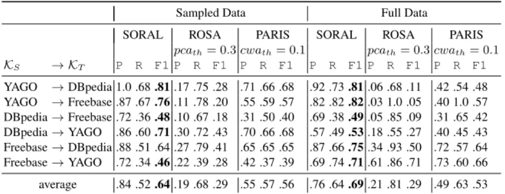
Sampled Data Full Data
SORAL ROSA PARIS SORAL ROSA PARIS pcath= 0.3 cwath= 0.1 pcath= 0.3 cwath= 0.1
KS → KT P R F1 P R F1 P R F1 P R F1 P R F1 P R F1 YAGO → DBpedia 1.0 .68 .81 .17 .75 .28 .71 .66 .68 .92 .73 .81 .06 .68 .11 .42 .54 .48 YAGO → Freebase .87 .67 .76 .11 .78 .20 .55 .59 .57 .82 .82 .82 .03 1.0 .05 .40 1.0 .57 DBpedia → Freebase .72 .36 .48 .10 .67 .18 .31 .50 .40 .69 .38 .49 .05 .85 .09 .31 .65 .42 DBpedia → YAGO .86 .60 .71 .30 .72 .43 .70 .66 .68 .57 .49 .53 .18 .55 .27 .40 .45 .43 Freebase → DBpedia .88 .51 .64 .27 .79 .41 .65 .65 .65 .87 .66 .75 .34 .93 .50 .72 .57 .64 Freebase → YAGO .72 .34 .46 .22 .39 .28 .42 .37 .39 .69 .74 .71 .61 .86 .71 .73 .60 .66 average .84 .52 .64 .19 .68 .29 .55 .57 .56 .76 .64 .69 .21 .81 .29 .49 .63 .53 Table 2:The performance of SORAL in comparison to the competing baselines.
7.1 Relation Alignment Accuracy
Sampling Configurations. Here, we show the impact of the sampling strategies on the candidate generation process. Through sampling we can efficiently perform the align-ment process in an online setting, and at the same time provide accurate results.
Table 1 shows the sampling strategies presented in Section 5.2. In the case of the stratified samplingwe construct the strata based on the DBpedia type taxonomy with a depth level from 2 up to 5 (DBpedia has a maximum depth level of 7). The results are averaged across the different KB pairs. Here we aim at finding the best parameter configuration for SORAL, specifically for: (i) sampling strategy, and (ii) sample size.
From Table 1 we see that the best performing strategy is based on the stratified sampling, with strata constructed at the depth level of three, and with a sample size of 500. With these two parameters, SORAL yields an F1 score of 0.64. We note a small fluctuation in terms of precision for the sample sizes of 500 and 1000. We check for statistical significance on the resulting F1 scores, however, the difference proved to be insignificant with a p − value = .17. On the other hand, we find statistical significance between the F1 scores for 100 and 500 entity samples (p − value = .01).
SORAL Effectiveness. Table 2 shows the results for the best configuration of SORAL (with stratified sampling at depth level 3) for the individual KB pairs. In the “Sampled Data” results group we compare SORAL against the competitors ROSA and PARIS. The results are highly significant when comparing SORAL against the competitors for the F1 score. In terms of precision, we have a relative improvement of 336% when compared to ROSA, whereas in the case of PARIS we have a 51% improvement. In terms of recall, we perform worse, however, given the low cwa and pca thresholds for our baselines leading to a low precision which makes such results hardly usable. Increasing the thresholds results an increase of precision, however, strongly penalizing the recall of the competitors.
In the group of results in column “Full Data”, we show the results of SORAL and the competitors when computed without sampling for the relation candidate generation. Here too we outperform the competitors to a large extent, with an average difference of 16% in terms of F1 for PARIS and even higher difference of 40% to ROSA.
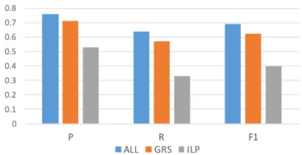
0 0.1 0.2 0.3 0.4 0.5 0.6 0.7 0.8 P R F1 ALL GRS ILP
Figure 2:Feature ablation for the different feature groups.
It is interesting to note that for SORAL on average we miss 13% of aligned rela-tions from the real coverage performance of SORAL when comparing the results with sampling and without. In terms of F1 measure we have only a small difference of 6%, which presents an optimal results when comparing the advantages we get in terms of efficiencythrough sampling.
Finally, we note varying performance of SORAL (with and without sampling) across the different KB pairs. For instance, in the case of YAGO → DBpedia we have perfect precision and the best F1 score. It is evident that DBpedia and YAGO represent high quality KBs, whereas Freebase is more noisy, thus, leading to a poorer performance. The main reason for such noise is that relations in Freebase are created by its users, and as such are not unique, in the sense that there are multiple relations representing similar concepts in Freebase.
From Table 2 we further notice that in the case of DBpedia to YAGO we have worse results when comparing the full against results obtained through sampling. This may be caused due to the difference in the number of statements per relation in the two KBs. DBpedia has a larger set of entity instances and statements per relation, and as such the ILP and GRS features are penalized more heavily in the full dataset. We believe that in this case the sampling plays a normalizing factor for such differences in terms of statements and the impact on the feature computation.
Feature Ablation. In the feature ablation we show as to what is attributed the perfor-mance of SORAL. Figure 2 shows the feature ablation results for the different feature groups in Section 5.3. The results are averaged across the different KB pairs and are computed based on models trained on the full data, such that we can assess the true power of the different groups.
The highest impact is attributed to the GRS feature group. This follows our intuition where we hypothesized that for a relation to be subsumed in a target relation, one of the important factors is the ability of rTto represent the entity instances. In other words, the
entity types for two relations should be similar. The next assumption we made was that ILPfeature scores, depending on the KB pairs, sometimes are insufficient, hence, the corresponding likelihood scores of the ILP measures can provide additional information on predicting correctly the label of a relation pair.
7.2 Query-Execution Overhead
Here we show the overhead in terms of time and network bandwidth usage for the sam-plingprocess. These represent important aspects considering that our relation alignment is setup in an online setting.
Time overhead. With respect to the time efficiency factor, we measured the time it takes to perform the different sampling strategies. The most efficient sampling strategy is first–N taking the least amount of time. The stratified sampling strategy requires the most amount of time, with a maximum of 3 seconds (for 1000 instances); a significantly higher execution time compared to other strategies. However, such an overhead for the task at hand is arguably not high.
Network bandwidth overhead. Understandably the amount of overhead in terms of bandwidth is uniformly distributed across the different sampling strategies. That is, considering that we sample for the same amount of entity instances. The highest amount of bandwidth overhead is introduced when we sample for 1000 entity instances, with a maximum 140 kb. In the performance evaluation of SORAL in Table 1, we found the optimal results to be with 500 entity sample instances, resulting in bandwidth overhead of 60 kb. This contrary to existing approaches that require the full content of a KB, represents a highly efficient way to compute such alignments.
8
Conclusion
We proposed SORAL, a relation alignment approach based on supervised machine learning approaches. We perform the specific task where for a given source relation rS we find relation subsumption in a target KB. Furthermore, we employ SORAL in
an online setting, where we ensure the efficiency of the proposed approach by extract-ing minimal samples of entity instances for a relation from the respective SPARQL endpoints. To ensure the accuracy of SORAL we computed features that range from association rule miningfeatures, to general statistics from relations.
References
1. Datasets by topical domain. http://linkeddatacatalog.dws.informatik. uni-mannheim.de/state/.
2. S. Auer, C. Bizer, G. Kobilarov, J. Lehmann, R. Cyganiak, and Z. G. Ives. DBpedia: A Nucleus for a Web of Open Data. In ISWC, 2007.
3. D. Aumueller, H.-H. Do, S. Massmann, and E. Rahm. Schema and ontology matching with coma++. SIGMOD, 2005.
4. C. M. Bishop. Pattern recognition and machine learning, volume 1. springer, 2006. 5. C. Bizer, T. Heath, K. Idehen, and T. Berners-Lee. Linked data on the Web. In WWW, 2008. 6. C. B¨ohm, G. de Melo, F. Naumann, and G. Weikum. Linda: distributed web-of-data-scale
entity matching. In CIKM, 2012.
7. I. F. Cruz, F. P. Antonelli, and C. Stroe. Agreementmaker: Efficient matching for large real-world schemas and ontologies. PVLDB, 2009.
8. M. d’Aquin, A. Adamou, and S. Dietze. Assessing the educational linked data landscape. In WebSci, 2013.
9. L. Dehaspe and H. Toivonen. Discovery of frequent datalog patterns. Data Mining and Knowledge Discovery, 1999.
10. R. Dhamankar, Y. Lee, A. Doan, A. Y. Halevy, and P. Domingos. imap: Discovering complex mappings between database schemas. In SIGMOD, 2004.
11. A.-H. Doan, J. Madhavan, P. Domingos, and A. Halevy. Ontology matching: a machine learning approach. Handbook of ontologies. International handbooks on information sys-tems. 2004.
12. L. Gal´arraga, N. Preda, and F. M. Suchanek. Mining rules to align knowledge bases. In AKBC, 2013.
13. L. Gal´arraga, C. Teflioudi, K. Hose, and F. M. Suchanek. Amie: association rule mining under incomplete evidence in ontological knowledge bases. In WWW, 2013.
14. P. Jain, P. Hitzler, A. P. Sheth, K. Verma, and P. Z. Yeh. Ontology alignment for linked open data. In ISWC, 2010.
15. T. Kirsten, A. Thor, and E. Rahm. Instance-based matching of large life science ontologies. In DILS, 2007.
16. M. Koutraki, N. Preda, and D. Vodislav. Sofya: Semantic on-the-fly relation alignment. In EDBT, 2016.
17. M. Koutraki, D. Vodislav, and N. Preda. Deriving intensional descriptions for web services. In CIKM, 2015.
18. S. Lacoste-Julien, K. Palla, A. Davies, G. Kasneci, T. Graepel, and Z. Ghahramani. Sigma: Simple greedy matching for aligning large knowledge bases. In KDD, 2013.
19. J. Madhavan, P. A. P. Bernstein, A. Doan, and A. Y. Halevy. Corpus-based Schema Matching. In ICDE, 2005.
20. R. J. Miller, L. M. Haas, and M. A. Hern´andez. Schema mapping as query discovery. In VLDB, 2000.
21. D. Movshovitz-Attias, S. E. Whang, N. Noy, and A. Halevy. Discovering subsumption rela-tionships for web-based ontologies. In Proceedings of the 18th International Workshop on Web and Databases, 2015.
22. R. Parundekar, C. A. Knoblock, and J. L. Ambite. Linking and building ontologies of linked data. In ISWC, 2010.
23. M. Schmachtenberg, C. Bizer, and H. Paulheim. Adoption of the linked data best practices in different topical domains. In ISWC. 2014.
24. L. Seligman, P. Mork, A. Y. Halevy, K. P. Smith, M. J. Carey, K. Chen, C. Wolf, J. Madhavan, A. Kannan, and D. Burdick. Openii: an open source information integration toolkit. In SIGMOD, 2010.
25. P. Shvaiko and J. Euzenat. Ontology matching: State of the art and future challenges. IEEE Trans. Knowl. Data Eng., 2013.
26. F. M. Suchanek, S. Abiteboul, and P. Senellart. Paris: Probabilistic alignment of relations, instances, and schema. PVLDB, 5(3), 2011.
27. F. M. Suchanek, G. Kasneci, and G. Weikum. YAGO: A core of semantic knowledge -unifying WordNet and Wikipedia. In WWW, 2007.
28. O. Udrea, L. Getoor, and R. J. Miller. Leveraging data and structure in ontology integration. In SIGMOD, 2007.
29. S. Wang, G. Englebienne, and S. Schlobach. Learning concept mappings from instance similarity. In ISWC, 2008.
30. D. T. Wijaya, P. P. Talukdar, and T. M. Mitchell. Pidgin: ontology alignment using web text as interlingua. In CIKM, 2013.