HAL Id: hal-03189296
https://hal-amu.archives-ouvertes.fr/hal-03189296
Submitted on 3 Apr 2021HAL is a multi-disciplinary open access archive for the deposit and dissemination of sci-entific research documents, whether they are pub-lished or not. The documents may come from teaching and research institutions in France or abroad, or from public or private research centers.
L’archive ouverte pluridisciplinaire HAL, est destinée au dépôt et à la diffusion de documents scientifiques de niveau recherche, publiés ou non, émanant des établissements d’enseignement et de recherche français ou étrangers, des laboratoires publics ou privés.
Distributed under a Creative Commons Attribution - NonCommercial| 4.0 International License
Liquid Cooling of a Microprocessor: Experimentation
and Simulation of a Sub-Millimeter Channel Heat
Exchanger
Julien Fontaine, J. Gonzales, Prashant Kumar, François Pigache, Pascal
Lavieille, Frédéric Topin, Marc Miscevic
To cite this version:
Julien Fontaine, J. Gonzales, Prashant Kumar, François Pigache, Pascal Lavieille, et al.. Liquid Cooling of a Microprocessor: Experimentation and Simulation of a Sub-Millimeter Channel Heat Exchanger. Heat Transfer Engineering, Taylor & Francis, 2019, 41 (15-16), �10.1080/01457632.2019.1628485�. �hal-03189296�
Liquid Cooling of a Microprocessor: Experimentation and Simulation of a
1
Sub-Millimeter Channel Heat Exchanger
2 3 4
Fontaine J.1, Gonzalez C.1,2, Kumar P.2, Pigache F. 1, Lavieille P. 1, Topin F. 2, Miscevic M. 1
5 6 7
1University of Toulouse, LAPLACE (Laboratory on Plasma and Conversion of Energy), Toulouse, France
8
2Aix Marseille Univ, CNRS, IUSTI, Marseille, France
9 10 11 12 13 14 15 16 17 18 19 20 21 22 23 24 25 26 27 28 29 30 31 32 33
Address correspondence to Dr. Marc Miscevic, University of Toulouse, LAPLACE, UPS-INP-34
CNRS, 118 Route de Narbonne, 31062 Toulouse Cedex 09, France. E-mail: 35
marc.miscevic@laplace.univ-tlse.fr 36
ABSTRACT
1
A heat exchanger dedicated to the cooling of a microprocessor has been designed and realized.
2
This heat exchanger consists of a bottom wall in contact with the processor and a cover that has
3
been dug to a depth of 200 μm on one side and 1 mm on the other side. Thus, by turning the
4
cover, the hydraulic diameter of the channel can be changed. Both hydraulic and thermal
5
performances of this heat exchanger have been experimentally tested. At the same time, 3D
6
numerical simulations were carried out on a model of the experimental prototype. Comparisons
7
between numerical and experimental results are in good agreement. In particular, the influence
8
of the distributor and the collector on the distribution of fluid flow and heat fluxes is emphasized.
9
A new concept of micro heat exchanger was then proposed for the cooling of electronics devices
10
for which wall to fluid heat exchange quality as well as pumping effect is very critical. In the
11
present work, the ability of a liquid heat exchanger involving a dynamic deformation of one of its
12
walls to cool a microprocessor is investigated. For that purpose, 3D transient numerical
13
simulations of fluid flow and conjugate heat transfer were performed using commercial software
14
based on the finite volume. Effect of geometrical and actuation parameters has been explored
15
demonstrating the ability of such heat exchanger to simultaneously pump the fluid and enhance
16
the heat transfer.
17 18
INTRODUCTION
1
The evacuation of the heat generated within a microprocessor is a crucial problem. It 2
affects the user from various points of view: limitation of performance and maximum allowable 3
temperature of the environment in which it can be used, drastic reduction in reliability and 4
lifetime, energy consumption of the chip. It is therefore necessary to develop efficient cooling 5
solutions even for high heat generation microprocessors and to keep it near its optimum operating 6
temperature. Numerous works have been conducted to propose new techniques to enhance heat 7
transfer and improve existing ones [1]. For application in high dissipative electronics, air-cooling 8
appears to be increasingly inappropriate due to low thermal conductivity as well as low density 9
and low heat capacity of this fluid. Thus, liquid or two-phase thermal management systems must 10
be developed. Furthermore, in addition to the rapid increase in the power density, electronic 11
packages are more and more miniaturized, implying to develop efficient cooling systems. Several 12
cooling solutions can then be envisaged. Among these solutions, micro channels-based heat 13
exchanger is often presented as one of promising cooling technologies [2-8]. For example, very 14
recently Kheirabadi and Groulx [8] have shown a device whose thermal resistance is varying 15
from 0.105 K/W to 0.08 K/W when the coolant (water) flowrate varies from 1.1 l/min to 3.8 l/min 16
in a microchannel heat sink in which channels were 0.5 mm wide and 2.3 mm tall. 17
Yang et al. [9] have proposed a general optimization process for the thermo-hydraulic 18
performances of mini-channel heat sinks. They reported empirical correlations extracted from 19
literature and gave some recommendations about their use for practical design. Although many 20
works have already been carried out, thermo-hydraulic behavior and performances of such 21
miniature heat sinks are still to be explored [10, 11]. 22
Among these micro channel-cooling systems, those equipped with corrugated channels 23
appear particularly interesting. Heat transfer and pressure drop in sinusoidal corrugated channels 24
have been studied by Nishimura et al. [12]. These authors showed that transition between laminar 1
and turbulent flows is obtained at lower Reynolds number (Re = 300) compared to straight 2
channel due to unsteady vortex motion. As for flat channel, the friction factor is inversely 3
proportional to Reynolds number in the laminar flow range, while it is independent of Reynolds 4
number in the turbulent one. Extending this study, Nishimura et al. [13] studied flow patterns 5
characteristics in symmetrical two-dimensional sinusoidal and arc-shaped corrugated channels at 6
moderate Reynolds numbers (20 < Re < 300). They concluded that the transitional Reynolds 7
number depends on the corrugation shape and is lower for the arc-shaped wall. 8
Niceno and Nobile [14] have conducted an extended numerical study on these corrugated 9
channels. They found that these two corrugation shapes are ineffective in terms of heat transfer 10
rate (slightly higher for sinusoidal compare to arc-shaped channel) as compared to flat channel in 11
steady low Reynolds flow. The unsteady regimes appear at different Reynolds numbers for the 12
two corrugation shapes: unsteady regime was observed at Re = 60 − 80 for arc-shaped channel 13
and at Re = 175 − 200 for sinusoidal one. On the other hand, heat transfer rate increases 14
significantly for both corrugation shapes, up to a factor of three, as a result of self-sustained 15
oscillations. Moreover, this transfer rate was found to be higher for arc-shaped channel while the 16
friction factor was smaller for sinusoidal channel. 17
Naphon [15] conducted a numerical study on various corrugation geometries arranged in 18
in-phase and out-phase layouts (e.g. flat plate, arc-shaped, trapezoidal and V-shaped) to enhance 19
the thermal performances. He obtained that for a given air flow rate, V-shaped corrugated 20
channel enhances most heat transfer. This enhancement is linked to boundary layer disruption. 21
Most of the studies revealed an increase in overall thermal performance from 3 to 5 times 22
depending on the working fluid. However, static corrugated channels have shown to increase 23
significantly the pressure drop. In such corrugated (and grooved) mini-channels, high heat 24
transfer usually leads to high Reynolds number (mostly turbulent) flow. 1
Yang et al. [16, 17] compared three different designs of a micro heat exchanger for use in a 2
liquid cooling system. Best thermal performances were obtained with the chevron channel heat 3
exchanger. Unfortunately, this heat exchanger was also the one generating the highest pressure 4
drops. 5
On the other hand, Léal et al. [18] proposed a relatively simple model of dynamic 6
corrugated mini-channel to be operated at low Reynolds number. This has been achieved by 7
deforming dynamically one of the channel walls. Very high heat transfer has been obtained 8
compared to static corrugated channel (with a relative gain in heat transfer coefficient of about 9
400%). It appeared to be the first study to introduce dynamic wall in such mini-channels heat 10
exchanger. 11
Very recently, Kumar et al. [19] extended this work and proposed a realistic 3D geometry 12
of dynamic corrugated heat exchanger. In their study, the average height of the channel is fixed 13
while the minimum gap (distance between the lowest point of the deformed wall and the fixed 14
wall) varies as a function of the relative amplitude. Numerical studies have been conducted for a 15
channel outlet pressure greater than the inlet one and for an imposed frequency of 50 Hz. They 16
showed that heat transfer coefficient is proportional to wave amplitude and that such devices 17
possess self-pumping capacity. This system can operate with negligible pressure drop, or even 18
without an external pump. 19
The aim of this paper is to determine the ability of this type of actuated liquid heat 20
exchanger to cool a micro-electronic device. First, a reference (static) heat exchanger has been 21
studied, from both experimental and numerical point of view. A systematic numerical study was 22
then conducted considering a micro-heat exchanger using three actuators to deform dynamically 23
one of its walls to understand the impact of operating parameters in enhancing thermo-hydraulic 24
characteristics. 1
2
REFERENCE HEAT EXCHANGER
3
Experimental setup 4
The reference exchanger consists of two parts, the sole made of copper and the cover made 5
of aluminum. Two grooves are machined in the sole and communicate with the inlet and outlet 6
pipes (see Figure 1). An O-ring is placed at the periphery for sealing. The cover is a simple 7
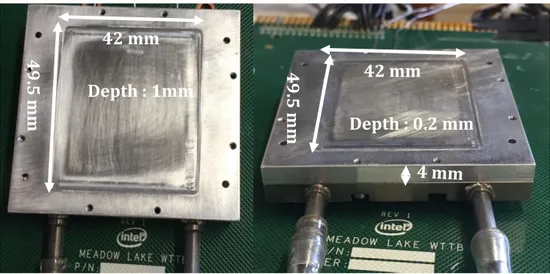
parallelepiped plate that has been dug to a depth of 200 μm on one face and 1 mm on the other. 8
Thus, by turning the cover, the hydraulic diameter of the channel can be changed. The channel 9
obtained for the circulation of the fluid after assembly is thus rectangular with a cross-section of 10
50 mm in width, 38 mm in length (distance between the distributor and the collector) and is 200
11
μm or 1 mm in height (Figure 2).
12
In order to be able to determine the thermal performance independently of the thermal 13
contact resistance between the exchanger and the microprocessor, three thermocouples were 14
inserted into the sole at a distance of 1 mm from the surface in contact with the liquid. These 15
thermocouples are K-type, sheathed in stainless steel, 500 µm in diameter. The holes in the sole 16
were made by electro erosion; they have a diameter of 600 µm and a length of 33 mm. Two other 17
identical thermocouples are placed in inlet and outlet pipes along with pressure taps (diameter 4 18
mm) in order to measure the inlet and outlet bulk temperatures of the fluid. All thermocouples
19
have been calibrated against a certified Pt100 RTD probe (accuracy of 0.05 °C). Thus, the 20
relative accuracy of temperature measurements is estimated at 0.1 ◦C. A differential pressure 21
sensor is positioned between the inlet and outlet pipes of the heat exchanger (the connections are 22
located 25 cm upstream and downstream of the heat exchanger) and allows measuring the 23
pressure loss with an accuracy better than 10 Pa. 24
The heat source is constituted by a microprocessor mock-up supplied by Intel Company 1
and fixed to the sole. This mock-up is geometrically identical to a commercially available 2
processor and generates similar and easily scalable thermal solicitations. 3
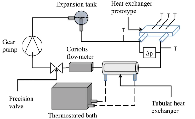
The heat exchanger is connected to a hydraulic circuit (see schema in Figure 3). A counter-4
current tubular heat exchanger is used as cold source for the fluid loop. The fluid then passes 5
through a Coriolis flowmeter allowing mass flow rate measurements in the range 0 up to 6 g/s 6
with an accuracy of 0.02 g/s. We thus obtained a maximum Reynolds number of 240 within the 7
heat exchanger for both considered thicknesses (hydraulic diameter respectively equal to 1960 8
µm and 398 µm). A variable speed gear pump is used for discharging the fluid into a precision
9
valve. This latter allows us to vary the pressure drop in the circuit at the desired value in a simple 10
manner. The fluid then flows toward the inlet of the heat exchanger prototype. A reservoir (open 11
to the atmosphere) is connected to the hydraulic circuit and serves as an expansion vessel. The 12
secondary fluid in this heat exchanger is thermostated water. 13
14
Numerical simulation 15
Simultaneously, direct numerical simulations of this heat exchanger were carried out using 16
commercial software Star- CCM+. The virtual prototype was constructed using the CAD model 17
of the assembly (bottom wall, top cover and channel). The conjugate heat transfer problem was 18
solved in the transient regime, and heat conduction is considered in all solid parts. Note that a 19
perfect thermal contact between top and bottom parts of the assembly was considered. For the 20
channel as well as inlet and outlet manifolds, incompressible laminar and transient flow and heat 21
transfer were solved using the classical combination of continuity, momentum and energy 22
equations (here simply written for constant properties): 23
𝛻⃗ ∙ 𝑢⃗ = 0 (1)
𝜌𝜕𝑢⃗⃗ 𝜕𝑡+ 𝜌(𝑢⃗ ∙ 𝛻⃗ )𝑢⃗ = 𝜌𝑔 − 𝛻⃗ ∙ 𝑃̿ + 𝜇𝛥𝑢⃗ (2) 1 𝜌𝐶𝑝( 𝜕𝑇 𝜕𝑡+ 𝑢⃗ ∙ 𝛻⃗ 𝑇) + 𝜌𝑢⃗ ∙ 𝜕𝑢⃗⃗ 𝜕𝑡+ 𝜌 2(𝛻⃗ ‖𝑢⃗ ‖ 2) ∙ 𝑢⃗ = 𝑘 𝑓𝛥𝑇 + 𝜕𝑃 𝜕𝑡+ ∅ (3) 2
Where ∅ is the volumetric energy source due to viscous dissipations. This term is taken into 3
account during all calculations; however, in the present work, it is negligible compared to the 4
wall heat transfer. 5
The physical properties of the fluid were considered to vary with the temperature (water 6
using the models of IAPWS-IF97 (International Association for the Properties of Water and 7
Steam, Industrial Formulation 1997) while the solid part properties are supposed constant (copper 8
for the base and aluminum for the top cover). The numerical resolution used a segregated 9
approach with implicit second order temporal discretization and ad hoc relaxations factors in 10
order to obtain adequate convergence behavior. 1 691 272 and 1 852 205 meshes were used for 11
the 1 mm and the 200 μm heat exchanger, respectively. For both cases, an unstructured trimmer -12
octree mesh type- is used in solid parts while structured hexahedral anisotropic cells are used in 13
the channel with 16 up to 20 cells along the height of the channel. This mesh is refined in the 14
vicinity of all solid-fluid interfaces and near inlet and outlet of the channel. Mesh convergence 15
effects were checked, and no additional improvement is obtained with further refinement. 16
Both mass flow rate and fluid temperature were imposed at the inlet of the heat exchanger; 17
outlet pressure is imposed at the atmospheric one. A uniform heat flux is imposed on the bottom 18
wall of the sole, on an area of 30x30 mm2 as in the experiments. The rest of the solid walls are 19
considered adiabatic (as experimental results show that thermal losses are negligible). 20
21
NUMERICAL ACTUATED PROTOTYPE
22
In the studied configuration, the lower wall was fixed and subjected to a constant heat flux 23
along the imprint of heating zone while the dynamically deformed upper wall (also called 1
"membrane" in the following) and side walls were kept adiabatic. Several actuators were 2
employed to dynamically deform the upper wall of a rectangular cross section micro-channel in 3
order to simultaneously enhance heat transfer and pump the fluid. 4
The length of the actuated zone (L) is 49 mm while width (W) is 35 mm. The channel gap 5
(g) is fixed and is 10 µm while the average height of the channel (𝛿) is linked to the wave 6
amplitude employed for wall deformation and the channel gap. The lengths of input and outlet 7
zones have been chosen long enough to establish the hydrodynamic. Furthermore, the no-slip 8
condition was imposed on the walls. 9
The influences of relative amplitude (A0), frequency (fr) and wavelength (𝜆) on
thermo-10
hydraulic performances are studied for an imposed value of the pressure difference between 11
outlet and inlet of the exchanger equal to zero. 12
Only three actuators were employed in the present study. The channel cross-section shape 13
is presented on Figure 4 where the actuator positions can be described using x1, x2, x3, x4, x5 and
14
x6. The positions x0 and x7 are fixed to external inlet and outlet zones as dampers. These small
15
zones make the fluid to enter and leave in laminar condition. The micro-channel geometry is 16
composed of four main parts: inlet zone, heated surface where the heat power is imposed, outlet 17
zone and membrane. This simplified geometrical configuration, dedicated to study the impact of 18
actuators operating parameters (3 actuators case) do include sidewall-damping effects on the 19
lateral side of the actuated zone. Along main flow axis the membrane displacement is linearly 20
interpolated between actuators pair and between actuator and fixed zone. 21
3D numerical simulations were carried out using the commercial software StarCCM+. This 22
software allows modeling fluid flow and heat transfer in dynamically deformed structures. The 23
flow was considered transient, three-dimensional and laminar. The working fluid was liquid 24
water (properties taken from IAPWS-97 at 27 °C) whose all thermo-physical properties were 1
supposed constant for systematic studies. The imposed heat power on the imprint (heated zone) 2
was 65 W (note that only half of the device is modeled due to symmetry). 3
The results presented focus on the "active zone" namely between S1 and S2 sections (see
4
Figure 4). All representative global thermo-hydraulic quantities were calculated in this zone. 5
The incompressible laminar and transient conjugate flow and heat transfer problems were 6
solved as for the static heat exchanger. The numerical resolution used a segregated approach with 7
implicit second order temporal discretization and ad hoc relaxations factors in order to obtain 8
adequate convergence behavior. The displacement of the top membrane is created by: 9
(1)- fixing it in inlet and outlet zone and displacing the upper wall at chosen height 10
(average height of the channel), 11
(2)- adding the movement of the three actuators (Eq. 4), 12
(3)- in between two actuators or one actuator and border, the displacement is simply 13
interpolated. 14
The displacement of actuator is given by the following equation for i=1,2,3 corresponding 15
to actuator along main flow axis: 16
𝐴𝑐𝑡𝑖 (𝑥, 𝑡) = 𝐴𝑜. 𝑐𝑜𝑠(2𝜋𝑓𝑟𝑡 + 𝛷𝑖) (4) 17
where 𝛷1 = 0°, 𝛷2, 𝛷3 are phase of actuators 𝐴𝑐𝑡1, 𝐴𝑐𝑡2 and 𝐴𝑐𝑡3, respectively.
18
In the studied configuration, the vertical plane passing through the central axis of the 19
channel is a plane of symmetry, so only half of the channel was simulated (i.e. W/2=17.5 mm). 20
The imposed power on the modeled half-imprint was thus 32.5 W to carry out numerical 21
simulations (see Figures 4 and 5). This allows us to reduce the number of mesh cells to optimize 22
computation time by dividing the simulated configuration by two compared to its actual size. 23
Note that the fluid flow was considered in x-direction while the width and height of the channel 24
were considered in y- and z-directions, respectively. 1
Meshing strategy was similar to the one used by Kumar et al. [19]. It was rather tricky to 2
create a convenient mesh in such highly anisotropic geometrical configuration subjected to large 3
amplitude deformations (up to 98 % of channel height) while keeping a computational time low 4
enough to carry out parametric study without sacrificing precision or convergence of the dynamic 5
transfer. 6
The deformed channel mesh is presented in Figure 5 in case of an actuator size of 11 mm 7
and a phase-shift between two consecutive actuators of 120° (=0°, -120°, -240°). 8
In case of dynamic corrugated channel, surface averaged and volume averaged thermo-9
hydraulic quantities for all operating configurations were calculated as follow. The Reynolds 10
number and hydraulic diameter are defined by: 11 𝑅𝑒 = 𝜌‖𝑢⃗⃗ ‖𝐷ℎ 𝜇 , 𝐷ℎ = 1 𝜆∫ 4𝑆 𝑝 𝑑𝜆 𝜆 0 (5) 12
Where S is the flow fluid passage area along the heated zone and p is the perimeter of the 13
passage section, respectively. Note that these quantities are averaged over a time period. 14
Following the method used in Léal et al. [18], the heat transfer coefficient is obtained by the 15
spatial and temporal averaged fluid temperature and wall temperature over the width and between 16
sections 𝑆1 and 𝑆2 (distance 𝐿) as well as over a period (𝜏=1/fr):
17 𝑇̅𝑤 = 1 𝜏𝑊𝐿∫ ∫ ∫ 𝑇𝑤(𝑥, 𝑦, 𝑡)𝑑𝑥 𝑑𝑦 𝑊 0 𝑑𝑡 𝑆2 𝑆1 𝑡+𝜏 𝑡 (6) 18 𝑇̅𝑚𝑓= 1 𝜏𝛿𝑊𝐿∫ ∫ ∫ ∫ 𝑇𝑚𝑓(𝑥, 𝑦, 𝑧, 𝑡)𝑑𝑥 𝑑𝑦 𝑊 0 𝑑𝑧 𝑧(𝑥,𝑡) 0 𝑑𝑡 𝑆2 𝑆1 𝑡+𝜏 𝑡 (7) 19
In the following, the global heat transfer coefficient and Nusselt number across the channel 20
(between S1 and S2) are defined as: 21 〈ℎ〉 = Γ (𝑇̅𝑤−𝑇̅𝑚𝑓) , 〈𝑁𝑢〉 = 〈ℎ〉 𝐷ℎ 𝑘𝑓 (8) 22
The calculations to test mesh convergence were performed for amplitude A0 = 85 μm and
1
frequency fr = 20 Hz. We initialized both corrugated shape and fluid flow. Then, calculations
2
were carried out until a periodic stationary regime is reached. This latter point is checked 3
comparing the temporal evolutions of global heat transfer and flow characteristics: calculations 4
were performed until the heat transfer coefficient values between two consecutive time periods 5
differs by less than 1 %. Consequently, an additional time period is added to extract all 6
instantaneous and time-averaged values of all physical quantities. 7
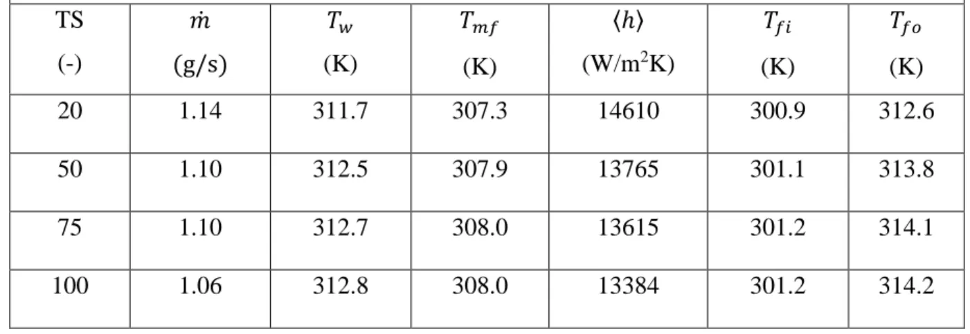
From the Table 1, it can be seen that reducing the characteristic mesh size from 3 to 2 mm 8
does not impact strongly on the global properties. The percentage differences between the 9
properties are respectively: 0.14 % for 𝑚̇, 0.0024 % for TW, 0.006 % for Tmf , 0.47 % for < h >,
10
0.0095 % for Tfi and 0.0095 % for Tfo. On increasing the mesh size, these quantities vary
11
significantly while reducing it further do not lead to any additional improvement. Based on these 12
observations and the percentage difference in the properties, we chose the BMS (Base Mesh Size) 13
equal to 2 mm to perform the systematic studies. 14
To perform the numerical simulations in terms of time effectiveness as well as the 15
precision, it is very important to obtain an optimized time step (TS). We test the following 16
number of time steps per period: 20, 50, 75 and 100. Based on these time steps, global 17
characteristics have been presented in Table 2. It can be observed that heat transfer coefficient 18
values decrease with increase in TS. On the other hand, ∆Tm=Tw−Tmf increases with increase in 19
TS.
20
In order to obtain an optimized TS value, we have calculated the percentage variation of 21
<h> and ∆Tm for different time steps based on the lowest value as a reference value for both
22
these quantities. When TS=50, we observed a variation of <h> equal to 2.84 % while the 23
variation in ∆Tm is 6.14 %. The global results of different characteristics do not vary strongly 24
when increasing TS. Moreover, higher value of TS increases the computational time while the 1
properties vary within a difference of 3 %. Hence, TS=50 has been chosen to study the impact of 2
different amplitudes and frequencies. 3
4 5
HYDRAULIC RESULTS 6
Hydraulic behavior of the reference heat exchanger 7
A first series of experimental tests and numerical simulations were carried out without 8
powering the processor, at a temperature of 20 ◦C, in order to characterize the heat exchanger 9
from hydraulic point of view. The pressure losses obtained as a function of the mass flow rate are 10
reported in Figure 6 for the two considered channel thicknesses (200 μm and 1 mm). Globally, 11
experiments and numerical simulations exhibit the same trend. Nevertheless, significant 12
discrepancies are found between experimental and numerical results, especially for the 1 mm 13
channel. These discrepancies can be explained by the fact that the pressure losses in the 14
numerical simulations are determined between the inlet and the outlet of the heat exchanger, 15
while in the experiments the tappings for the pressure measurement are located at 25 cm upstream 16
and 25 cm downstream of the prototype. Thus, additional pressure losses are taken into account in 17
the experiments (regular pressure drop in the inlet and outlet tubes, as well as singular pressure 18
drops in the connections between the tubes of the loop and the heat exchanger). 19
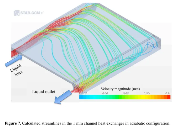
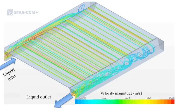
Furthermore, in the 1 mm channel heat exchanger, the flow distribution appears less 20
homogeneous than in the 200 μm channel heat exchanger, as it can be seen in Figures 7 and 8, 21
respectively. Such a flow maldistribution variation according to the channel hydraulic diameter is 22
not surprising: it has widely been highlighted. For example, Kheirabadi and Groulx [4] 23
numerically calculated variation of the mean velocity from a channel to another in an array of 24
parallel microchannels connected to a single manifold at the inlet and at the outlet. Variation up 1
to 52 % was highlighted for the 1 mm microchannel width, while this variation was only 16 % for 2
the 0.25 mm microchannel width. In the present study, the flow distribution in the 1 mm channel 3
heat exchanger could be homogenized by optimizing the distributor and collector headers as 4
suggested, for instance, by Saeed and Kim [20]. From these figures, it can be speculated that the 5
main part of the pressure drop in the 200 μm channel heat exchanger is the regular pressure drop 6
in the channel itself, while in the 1 mm the main part of the pressure drop corresponds to the 7
pressure drop in the singularities and in the manifolds. 8
To assess the respective contributions of the channel and the singularities on the total 9
pressure drop, an analytical estimation can be done. Assuming a Poiseuille flow in the inlet and 10
outlet tubes, as well as in the channel, the pressure drop can be calculated as: 11 Δ𝑝 = 64 𝑅𝑒𝐷𝑡 𝐿𝑡 𝐷𝑡 1 2𝜌𝑈𝑡 2+ 64 𝑅𝑒𝐷ℎ 𝐿𝑐 𝐷ℎ 1 2𝜌𝑈𝑐 2+ ∑ 𝜉 𝑖 1 2𝜌𝑈𝑐 2 𝑖 (10) 12 With: 13 𝑅𝑒𝐷𝑡 = 𝜌𝑈𝑡𝐷𝑡 𝜇 , 𝑅𝑒𝐷ℎ = 𝜌𝑈𝑐𝐷ℎ 𝜇 𝑤𝑖𝑡ℎ 𝐷ℎ = 4𝑒𝑙 2(𝑒+𝑙)≈ 2𝑒 14
The last term in equation 10 represents the pressure drop due to all the singularities. The 15
value of ∑𝑖𝜉𝑖 is adjusted to reproduce the experimental pressure drop of the 1 mm channel heat 16
exchanger: ∑𝑖𝜉𝑖 ≈ 5.
17
The global pressure losses of the device equipped with the 200 µm channel heat exchanger 18
are 2 to 2.5 times higher than those measured with the one using the 1 mm channel heat 19
exchanger, while the hydraulic diameter is 5 times lower. This behavior can be explained by 20
analyzing the part of the regular pressure losses in comparison with the singular pressure losses 21
corresponding to the different changes in flow direction and cross-sections. These relative 22
contributions are shown in Figure 10. For the 1 mm channel heat exchanger, the pressure losses in 23
the actual channel are negligible, less than 2 % of the total pressure losses. For the 200 µm 1
channel, these pressure losses in the channel become preponderant and represent 60 to 70 % of 2
the total pressure losses. The superimposed graph on Figure 10 compare the numerical pressure 3
drop along each minichannel with the theoretical values deduced from established Poiseuille flow 4
model. A fair agreement is obtained in both case, the numerical value being globally about 10 % 5
higher than the theoretical one, this is due to the inlet-outlet effect along with maldistribution. 6
7
Hydraulic behavior of the virtual dynamic prototype 8
Local fields are presented for the dynamic heat exchanger with A0 = 100 μm and fr = 10 Hz
9
for arbitrary time during periodic stationary regime. During expansion of the dynamic channel, 10
the fluid moves in the longitudinal direction because of the successive expansion and 11
contractions. Wall movement induces also vertical (i.e. towards heated wall) displacement of the 12
fluid. Characteristic times associated to vertical and horizontal fluid displacement are similar and 13
significantly lower than the actuation one. 14
Mass flow rate is proportional to both frequency and amplitude. High frequency leads to 15
fast movement of the corrugated wall, which in turn enhances the mass flow. The latter is 16
therefore directly proportional to the frequency (Figure 12 top). Increasing amplitude (at constant 17
gap) leads to increase the channel volume thus to have more fluid in the channel. This behavior 18
also enhances mass flow rate in the system, which is also directly proportional to the amplitude 19
(Figure 12 bottom). Note that increasing amplitude at constant gap adds mainly volume to the 20
channel near the membrane and increases average height. 21
Influence of gap size has been tested on mass flow rate and heat transfer for amplitude 100 22
μm and frequency 10 Hz. The initial gap was fixed at 10 μm and then varied up to 35 μm. On
23
Figure 13, it can be easily observed that mass flow rate decreases with increasing gap. This 24
indicates that global efficiency of such device is largely affected by the minimum constriction 1 height. 2 3 THERMAL PERFORMANCE 4
Reference heat exchanger 5
In order to determine the heat performance of the two configurations of the heat exchanger, 6
specific tests were carried out. The experimental protocol consists in imposing a water flow rate 7
by means of the gear pump and then supplying the microprocessor simulator with an electrical 8
power such that the water temperature difference between the inlet and the outlet is equal to 9
10±0.2 ◦C. The inlet temperature of the water in the exchanger is imposed at 23.5 ◦C for all the
10
tests. The deviations between the applied electric power and the heat flux received by the water 11
(quantified by multiplying the mass flow rate with the enthalpy variation) vary between 0 and 7 12
% and are on average 4 %.
13
The mean temperature <Tw> of the bottom wall of the heat exchanger is evaluated by
14
performing a 2nd order polynomial regression of the measured wall temperatures and then 15
integrating this regression between the inlet and the outlet of the channel (i.e. between the outlet 16
of the distributor and the inlet of the collector, on a distance of 38 mm). It should be noted that 17
this calculation represents only an estimation of the mean temperature because it does not take 18
into account the 2D distribution of the surface temperature (variation in the direction 19
perpendicular to the main axis of the flow). The average fluid temperature <Tf> is estimated by
20
performing an arithmetic mean between the inlet and outlet water bulk temperatures. Considering 21
the operating conditions described above, this average temperature of the water in the heat 22
exchanger is substantially constant for all the experiments and is equal to 28.5 ◦C. An ”apparent” 23
overall thermal conductance G of the heat exchanger is then defined as: 1
𝐺 =𝑚̇𝑐〈𝑇𝑝(𝑇𝑜𝑢𝑡−𝑇𝑖𝑛)
𝑤〉− 〈𝑇𝑓〉 (11)
2
The variations of this apparent overall thermal conductance as a function of the mass flow 3
rate are shown in Figure 14 for both considered channel thickness. 4
As it can be seen from this figure, the thermal conductance of the 200 μm channel heat 5
exchanger is substantially higher than that of the 1 mm one: enhancement up to 70 % is achieved 6
for mass flow rate approximately equal to 3 g/s. For such a mass flow rate, the overall thermal 7
conductance of the 200 μm channel heat exchanger is almost 15 W/K. 8
Let’s consider 3 typical application cases using water as the working fluid, and a maximum 9
allowable fluid temperature difference of 10 °C between inlet and outlet. The severe environment 10
case will impose a cold source at a temperature relatively close to the maximum allowable 11
processor temperature (e.g. 70 °C) along with limitations on the flowrate. In such conditions, heat 12
flux up to 125 W can be removed from the microprocessor with a mass flowrate of 3 g/s. The 13
temperature of the bottom wall of the heat exchanger would be only about 8 °C higher than the 14
fluid mean temperature. For a mass flow rate of about 5.4 g/s up to 225 W could be removed with 15
a wall to fluid temperature difference of less than 20 °C (e.g. automotive applications). Finally, 16
increasing the mass flow rate up to 9 g/s, the actuated channel allows to extract 375 W with a wall 17
to fluid temperature of 30 °C. This device is thus also an efficient solution for data center type 18
applications. Moreover, contrarily to static mini/microchannels which generate prohibitory high 19
pressure drop and fluid maldistributions when operated in parallel, the active heat exchanger -due 20
to the pumping effect- constitute a best suited device for low pressure losses and well-distributed 21
flow in parallel branches of a fluid network. It can thus be concluded that such a heat sink can be 22
efficiently integrated to the different constraints of applications involving microprocessor thermal 23
management. 1
Numerical simulations have been performed in the same conditions than the experiments 2
(i.e. inlet water temperature equal to 23.5 ◦C, heat flux adjusted to obtain a temperature 3
difference between inlet and outlet of 10 ◦C). Virtual temperature sensors are placed at the same 4
locations than the experimental ones and data are extracted from the numerical temperature field. 5
The same procedure than - used in the experiments is then applied to calculate the apparent 6
overall thermal conductance; numerical results are reported along with experimental ones (Figure 7
14). 8
Adequacy between experimental and numerical results is excellent for the 200 μm channel 9
heat exchanger, while the numerical simulations slightly overestimate the overall thermal 10
conductance in the case of the 1 mm channel heat exchanger. As mentioned in the hydraulic 11
behavior section, the flow in the 1 mm channel is non-uniformly distributed. This maldistribution 12
of the flow implies that the temperature field of the fluid is farther from a one-dimensional field 13
than in the case of the 200 μm channel (see Figures 15 and 16). Calculating the mean temperature 14
of the fluid by integrating a second order polynomial trend curve as described above is therefore 15
less precise in the case of the 1 mm channel than in the case of the 200 μm channel. In the case of 16
the 1 mm channel heat exchanger, the flow field is more sensitive to the deviation in the imposed 17
inlet conditions and geometry compared to the real ones. It is thus not surprising to obtain a better 18
match between numerical results and experiments in the case of the best-distributed flow. 19
20
Numerical prototype 21
Due to movement of the channel wall, cold fluid is moved near the heated wall successively 22
at every location; this boundary layer disruption increases sharply heat transfer along with mixing 23
that takes place within the core flow. On temperature field, successive hot and “cold” plumes” 1
could be seen (Figure 17). Near inlet cold fluid fill the pocket during expansion, then is driven 2
toward heated surface, and eventually transferred below the next actuated zone. The constricted 3
zone acts as a barrier separating inlet and outlet parts. This leads the fluid to fill expansion zone 4
while being mixed efficiently; it is then transferred in the next pocket over time. These ”bursts” 5
repeat cyclically along with mixing thus increasing heat transfer. 6
Heat transfer coefficient depends on both imposed frequency and amplitude. Increasing 7
frequency increases the mixing effect and the fluid velocity. Thus, it results in high heat transfer 8
coefficients varying roughly proportionally to the frequency (see Figure 18.a). On the other hand, 9
increasing amplitude -while keeping the gap (minimum height below actuators) constant- leads to 10
increase the average height of the channel and thus reduces the heat transfer coefficient. This one 11
is thus found to decrease linearly with the amplitude (see Figure 18.b). Nevertheless, the heat 12
transfer coefficient remains very high (greater than 10 000 W/m2K) for all tested cases. This is
13
due two main effects: the average fluid thickness increases, and the fluid velocities decrease. 14
Mainly the most constricted zones become less and less efficient as the gap increases. As these 15
zone (which cross all the channel length) are the place where the most efficient heat transfer takes 16
place, it is not surprising to observe a net decrease in heat transfer coefficient. Two main 17
conclusions could be drawn from these results: although the heat transfer coefficient decreases 18
when increasing channel height, for sub-millimeter cases it remains high enough to produce a 19
very small thermal resistance compared to the other involved in a chip cooling assembly (e.g. 20
contact resistances...). As, the flow increases with channel height, the need to remove relatively 21
high power with limited inlet-outlet temperature difference will by a more important design 22
parameter. Moreover, required pumping power and mechanical effort and constraints will be 23
more easily meet for channel with ”large” dimensions i.e. going more toward one millimeter than 24
100 μm.
1
A global thermal conductance of the virtual prototype can be derived from these heat 2
transfer coefficient values. The variation of this conductance is reported on Figure 19 along with 3
the experimental ones of the reference heat exchanger for both 1 mm and 200 µm channel 4
thickness. When the channel wall is actuated a sharp heat transfer enhancement is obtained: for a 5
mass flow rate of 1 g/s the thermal conductance of the virtual prototype is almost the triple than 6
the one of the 200 µm reference heat exchanger (corresponding thus to an enhancement of 7
approximately 200 %). For a mass flow rate of 3 g/s the enhancement is almost 100 %. 8
The thermal conductance of the virtual prototype appears thus very high. for example, as a 9
comparison point, [8] have developed several prototypes of very compact heat exchangers for the 10
cooling of electronics. They obtained a thermal conductance of 26 W/K considering a serpentine 11
channel with a mass flow rate of 18 g/s (leading to a pressure drop of 14 700 Pa). These thermal 12
conductance is very close from the one obtained with the virtual prototype with a mass flow rate 13
of 3 g/s (with an imposed zero pressure difference). So, the actuated heat exchanger appears as a 14
good candidate when efficient cooling is needed. 15
16
CONCLUSION 17
An experimental setup and a numerical tool have been built in order to analyze 18
hydrothermal performances of heat sink with low diameter channel. For the 1 mm channel heat 19
exchanger, it was found that the main contribution in the pressure drop is due to the singularities 20
and the tubes upstream and downstream of the heat exchanger, and that the flow is badly 21
distributed in the channel. For the 200 μm channel, the main contribution in the pressure drop is 22
due to the pressure loss in the channel itself, and the maldistribution is not significant. From heat 23
transfer point of view, the 200 μm channel heat exchanger allows reaching thermal conductance 24
up to 15 W/K with a very low mass flow rate of 3 g/s. This thermal performance demonstrates 1
that such a liquid cooling heat sink could be efficiently used for the thermal management of 2
electronic chip like microprocessor. Nevertheless, important improvements in the thermo-3
hydraulic performance could be obtained by optimizing the internal design. 4
Integration of the pumping function within a heat exchanger can be obtained considering 5
dynamic morphing of at least one of the wall of this heat exchanger. In addition, this dynamic 6
morphing may conduct to a significant heat transfer enhancement, making the concept 7
particularly interesting for embedded thermal management systems. A numerical tool has been 8
developed that allows determining the thermo-hydraulic performances of such a heat exchanger. 9
To meet the application constrains, the dynamic deformation has to be realized with a small 10
number of actuators. So, only 3 actuated zones are considered in the present work. It has then 11
been established that: 12
- The mass flow rate is mainly controlled by the frequency and amplitude of the 13
deformation, as well as the gap; 14
- High heat transfer coefficient values can be obtained, up to 20 000 W/m2K;
15
- The corresponding thermal conductance variation according to the mass flow rate is 16
almost twice the one of the 200 μm reference static heat exchanger. In addition to the integration 17
of the pumping function within the heat exchanger, important heat transfer enhancement is thus 18 obtained. 19 20 NOMENCLATURE 21 22
𝐴𝑜 relative amplitude, dimensionless 23
𝐶𝑝 specific thermal capacity, J.kg-1.K-1
24
𝐷ℎ hydraulic diameter, m 25
𝑓𝑟 frequency, Hz 1
𝑔 minimum gap of the channel, m
2
ℎ mean heat transfer coefficient at the heated wall, W.m-2.K-1
3
〈ℎ〉 global heat transfer coefficient at the heated wall, W.m-2.K-1 4
𝑘𝑓 fluid thermal conductivity, W.m-1.K-1 5
𝐿 imprint length of heated zone, m 6
𝑚̇ mass flow rate, kg.s-1 7
𝑞 heat flux, W.m-2 8
𝑃𝑔 pressure gain in actuated zone, Pa
9
𝛥𝑃 pressure difference between outlet-inlet sections, Pa 10
𝑃𝑃 pumping power, W
11
𝑝 perimeter of the channel passage, m 12
𝑆 exchange surface, m2
13
𝑡 time, s
14
𝑇̅𝑓𝑚 mean fluid temperature at a given axial position, K 15
〈𝑇̅𝑓𝑚〉 mean fluid temperature in the channel, K
16
𝑇̅𝑤 mean wall temperature on a heated zone, K
17
〈𝑇̅𝑤〉 mean wall temperature in the actuated zone, K 18 ‖𝑢⃗ ‖ average velocity, m.s-1 19 𝑊 channel width, m 20 Special characters
𝛿 average distance between walls, m 21
Γ total solid to fluid heat transfer, W 22
∅ volumic heat source, W.m-3 23
𝜌 fluid density, kg.m-3
24
𝜆 wavelength, m
25
𝜔 number of waves per unit length, m-1 26
𝜇 dynamic viscosity, kg.m-1.s-1 27
𝜉 pressure drop coefficient, dimensionless 28
𝜏 period, s
1
ACKNOWLEDGMENT 2
This work has been realized in the framework of the CANOPEE project and supported by 3
the ”Fond Unique Interministériel (FUI) - 18th call for projects”. We gratefully acknowledge 4
contributions from all project partners. 5
6
REFERENCES
7
[1] Léal L., Miscevic M., Lavieille P., Amokrane M., Pigache F., Topin F., Nogarède B., and 8
Tadrist L., An overview of heat transfer enhancement methods and new perspectives: focus on 9
active methods using electroactive materials, Int. J. Heat Mass Transf., vol. 61, pp. 505-524, 10
2013 11
[2] Xie X.L., Liu Z.J., He Y.L., and Tao W.Q., Numerical study of laminar heat transfer and 12
pressure characteristics in a water-cooled minichannel heat sink, Applied Thermal Engineering, 13
vol. 29, pp. 64-74, 2009 14
[3] Tullius JF., Vajtai R., and Bayazitoglu Y., A review of cooling in microchannels, Heat 15
Transfer Engineering, vol. 32, no. 7-8, pp. 527-541, 2011.
16
[4] Kheirabadi A.C., and Groulx D., A comparison of numerical strategies for optimal liquid 17
cooled heat sink design, Proceedings of the ASME 2016 Summer Heat Transfer Conference, 18
Paper HT2016-7076, July 10-14, Washington DC, USA, 2016. 19
[5] Kheirabadi A.C., and Groulx D., Cooling of server electronics: a design review of existing 20
technology, Applied Thermal Engineering, vol. 105, pp. 622-638, 2016. 21
[6] Sohel Murshed S.M., and Nieto de Castro C.A., A critical review of traditional and emerging 22
techniques and fluids for electronics cooling, Renewable and Sustainable Energy Reviews, vol. 23
78, pp. 821-833, 2017. 24
[7] Habibi Khalaj A., and Halgamuge S.K., A Review on efficient thermal management of air- 1
and liquid-cooled data centers: From chip to the cooling system, Applied Energy, vol. 205, pp. 2
1165-1188, 2017. 3
[8] Kheirabadi A.C., and Groulx D., Experimental evaluation of a thermal contact liquid cooling 4
system for server electronics, Applied Thermal Engineering, vol. 129, pp. 1010-1025, 2018. 5
[9] Yang X.H., Tan S.C., Ding Y.J., and Liu J., Flow and thermal modeling and optimization of 6
micro/mini-channel heat sink, Applied Thermal Engineering, vol. 117, pp. 289-296, 2017. 7
[10] Dixit T., and Ghosh I., Review of micro- and mini-channel heat sinks and heat exchangers 8
for single phase fluids, Renewable and Sustainable Energy Reviews, vol. 41, pp. 1298-1311, 9
2015. 10
[11] Ghani I.A., Sidik N.A.C., and Kamaruzaman N., Hydrothermal performance of 11
microchannel heat sink: The effect of channel design, International Journal of Heat and Mass 12
Transfer, vol. 107, pp. 21-44, 2017.
13
[12] Nishimura, T., Ohori, Y., and Kawamura, Y., Flow characteristics in a channel with 14
symmetric wavy wall for steady flow, Journal of Chemical Eng. of Japan, Vol., 17, no. 5, pp. 15
466- 471, 1984. 16
[13] Nishimura, T., Murakami, S., Arakawa, S., and Kawamura, Y., Flow observations and mass 17
transfer characteristics in symmetrical wavy-walled channels at moderate Reynolds numbers for 18
steady flow, International Journal of Heat and Mass Transfer, Vol. 33, no. 5, pp. 835-845, 1990. 19
[14] Niceno, N., and Nobile, E., Numerical analysis of fluid flow and heat transfer in periodic 20
wavy channels, International Journal of Heat and Fluid Flow, Vol. 22, pp. 156-167, 2001. 21
[15] Naphon, P., Effect of wavy plate geometry configurations on the temperature and flow 22
distributions, International Com. On Heat and Mass Transfer, Vol. 36, pp. 942-946, 2009. 23
[16] Yang C.Y., Yeh C.T., Liu W.C., and Yang B.C., Advanced micro-heat exchangers for high 24
heat flux, Heat transfer Engineering, vol. 28, no. 8-9, pp. 788-794, 2007. 1
[17] Yang C.Y., and Liu W.C, Development of a mini liquid cooling system for high-heat-flux 2
electronic devices, Heat Transfer Engineering, vol. 32, no. 7-8, pp. 690-696, 2011. 3
[18] Léal, L., Topin, F., Lavieille, P., Tadrist, L., and Miscevic, M., Simultaneous integration, 4
control and enhancement of both fluid flow and heat transfer in small scale heat exchangers: A 5
numerical study, International Com. onn Heat and Mass Transfer, vol. 49, pp. 36-40, 2013. 6
[19] Kumar, P., Schmidmayer, K., Topin, F., and Miscevic, M., Heat transfer enhancement by 7
dynamic corrugated heat exchanger wall: Numerical study, Journal of Physics: Conference 8
Series, vol. 745, pp. 32-61, 2016.
9
[20] Saeed M., and Kim M.H., Header design approaches for mini-channel heatsinks using 10
analytical and numerical methods, Applied Thermal Engineering, vol. 110, pp. 1500-1510, 2017. 11
1 2
Table 1. Presentation of global thermal and flow properties for different mesh sizes for number of time step per period TS=50.
BMS 𝑚̇ (g/s) 𝑇𝑤 (K) 𝑇𝑚𝑓 (K) 〈ℎ〉 (W/m2K) 𝑇𝑓𝑖 (K) 𝑇𝑓𝑜 (K) 3 mm 1.11 312.51 307.87 13829 301.1 313.8 2 mm 1.10 312.51 307.85 13765 301.1 313.8 3 4 5 6 7
1
Table 2. Presentation of global thermal and flow properties for different time steps for a characteristic mesh size BMS=2 mm
TS (-) 𝑚̇ (g/s) 𝑇𝑤 (K) 𝑇𝑚𝑓 (K) 〈ℎ〉 (W/m2K) 𝑇𝑓𝑖 (K) 𝑇𝑓𝑜 (K) 20 1.14 311.7 307.3 14610 300.9 312.6 50 1.10 312.5 307.9 13765 301.1 313.8 75 1.10 312.7 308.0 13615 301.2 314.1 100 1.06 312.8 308.0 13384 301.2 314.2 2 3 4
1 2 3
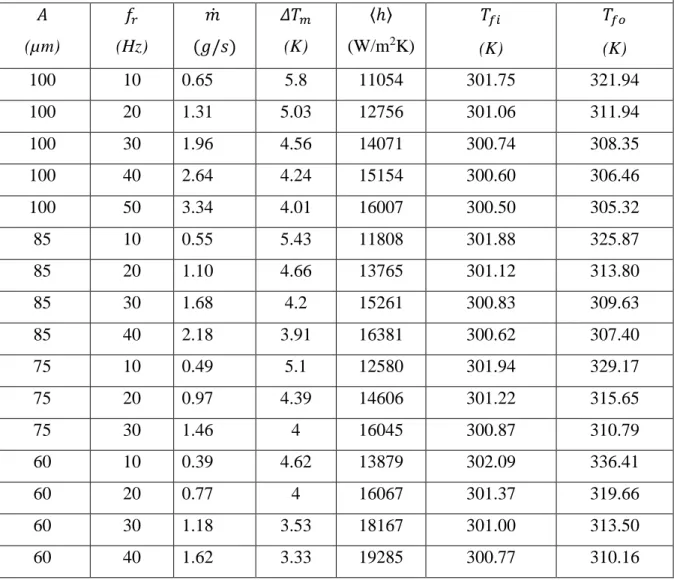
Table 3. Presentation of operating parameters (wave amplitude and frequency) on mass flow rate, surface and mean fluid temperature difference, heat transfer coefficient, inlet and outlet fluid temperatures.
𝐴 (µm) 𝑓𝑟 (Hz) 𝑚̇ (𝑔/𝑠) 𝛥𝑇𝑚 (K) 〈ℎ〉 (W/m2K) 𝑇𝑓𝑖 (K) 𝑇𝑓𝑜 (K) 100 10 0.65 5.8 11054 301.75 321.94 100 20 1.31 5.03 12756 301.06 311.94 100 30 1.96 4.56 14071 300.74 308.35 100 40 2.64 4.24 15154 300.60 306.46 100 50 3.34 4.01 16007 300.50 305.32 85 10 0.55 5.43 11808 301.88 325.87 85 20 1.10 4.66 13765 301.12 313.80 85 30 1.68 4.2 15261 300.83 309.63 85 40 2.18 3.91 16381 300.62 307.40 75 10 0.49 5.1 12580 301.94 329.17 75 20 0.97 4.39 14606 301.22 315.65 75 30 1.46 4 16045 300.87 310.79 60 10 0.39 4.62 13879 302.09 336.41 60 20 0.77 4 16067 301.37 319.66 60 30 1.18 3.53 18167 301.00 313.50 60 40 1.62 3.33 19285 300.77 310.16 4 5
List of figure captions
1 2
Figure 1. Picture of the bottom wall of the heat exchanger, made of copper. The two grooves 3
constitute the manifolds. 4
Figure 2. Pictures of the heat exchanger after assembly: - left : top view (dug cover) - right : side 5
view. Dimension of the grooved part (42 x 49. 5 mm ; thickness 1 mm (left) and 0.2 mm (right) 6
Figure 3. Sketch of the experimental apparatus. 7
Figure 4. Cross-section of dynamically corrugated micro-channel. The lower wall is subjected to 8
constant heat flux between x1 and x7, the gap g is the minimum height of the channel. Upper 9
profiles are drawn for 2 different amplitudes and same gap 10
Figure 5. Mesh view micro-channel at an arbitrary time. Dimension in the z-direction is 11
magnified 50 times. The bottom wall is uniformly heated below the actuated zone (fine mesh), all 12
other walls are kept adiabatic. 13
Figure 6. Experimental and numerical pressure losses as a function of the mass flow rate for the 14
two channel thicknesses. 15
Figure 7. Calculated streamlines in the 1 mm channel heat exchanger in adiabatic configuration. 16
The liquid temperature is 20 °C. Blue: 0 - Red 0.1 m/s. 17
Figure 8. Calculated streamlines in the 200 µm channel heat exchanger in adiabatic 18
configuration. The liquid temperature is 20 °C. Blue: 0 - Red 0.25 m/s. 19
Figure 9. Variation of the pressure loss in the heat exchangers as a function of the mass flow 20
rate. The symbols are the results obtained experimentally; The lines are the results given by Eq. 21
10 with ∑𝑖𝜉𝑖 = 5.
22
Figure 10. Comparison between regular and singular pressure drops in the 1 mm channel (top) 23
and 200 µm channel (bottom) heat exchanger. ∆ptube represents the pressure drop in the 25 cm
24
upstream and 25 cm downstream tube. 25
Figure 11. Instantaneous velocity field: for A0=100 µm and fr=10 Hz. Color range (Blue : 0 -
1
Red 1 m/s). The vertical scale is magnified 100 times. Channel height is 10 µm below center 2
actuator and total length is 7 cm. 3
Figure 12. Influence of (top) Frequency for A0 = 100 µm and, (bottom) Amplitude for fr=10 Hz
4
on mass flow rate. 5
Figure 13. Influence of gap size on mass flow rate for A0 = 100 µm and fr=10 Hz.
6
Figure 14. Variation of the apparent thermal conductance as a function of the mass flow rate for 7
the two channel thicknesses. The same procedure is applied to calculate G (eq. 8) from the 8
experiments and the numerical simulations; the maximum uncertainty is evaluated at 8%. 9
Figure 15. Temperature field of the water at mid-height of the 200 µm channel. The inlet 10
temperature is 23.5 °C, the mass flow rate is 1.5 g/s and the heat flux is 62.7 W. 11
Figure 16. Temperature field of the water at mid-height of the 1 mm channel. The inlet 12
temperature is 23.5 °C, the mass flow rate is 1.5 g/s and the heat flux is 62.7 W. 13
Figure 17. Instantaneous temperature field for A0=100 µm and fr = 10 Hz. Vertical scale is
14
magnified 100 times. Cold fluid fills the space below 1st actuator (here ascending) with small
15
backflow due to the 2d actuator "pressing" the fluid on surface (height is about 50 µm). The fluid 16
is mainly driven toward 3rd actuator and outlet. 17
Figure 18. Influence of (a) Frequency for A0=100 µm and, (b) Amplitude for fr = 10 Hz on heat
18
transfer coefficient. 19
Figure 19. Thermal conductance as a function of the mass flow rate: comparison between the 20
numerical actuated prototype with A0=100 µm, the 200 µm and the 1 mm reference static heat
21
exchangers. 22
1 2 3 4 5 6
Figure 1. Picture of the bottom wall of the heat exchanger, made of copper. The two grooves 7
constitute the manifolds. 8 9 10 11
Coola
nt flo
w
42 mm1
2
3 4
Figure 2. Pictures of the heat exchanger after assembly: top cover and bottom plate placed over a 5
CPU Thermal test Vehicle - left : top view (dug cover) - right : side view. Dimension of the 6
grooved part (42 x 49. 5 mm ; thickness 1 mm (left) and 0.2 mm (right). 7 8 9 10 42 mm 4 9 .5 mm Depth : 1mm 42 mm 4 9 .5 mm Depth : 0.2 mm 42 mm 4 9 .5 mm Depth : 1mm 42 mm 4 9 .5 mm Depth : 0.2 mm
1
2 3
4 5
Figure 3. Sketch of the experimental apparatus. 6 7 8
∆p
Gear
pump
Expansion tank
Prototype of
heat exchanger
Counter-current
tubular heat
exchanger
Coriolis
flowmeter
Precision
valve
T
T
T T T
Thermostated
bath
Expansion tank
Heat exchanger
prototype
Thermostated bath
Gear
pump
Precision
valve
Coriolis
flowmeter
Tubular heat
exchanger
1 2 3 4 5 6
Figure 4. Cross-section of dynamically corrugated micro-channel. The lower wall is subjected to 7
constant heat flux between x1 and x7, the gap g is the minimum height of the channel. Upper 8
profiles are drawn for 2 different amplitudes and same gap 9
10 11
1 2
3
Figure 5. Mesh view micro-channel at an arbitrary time. Dimension in the z-direction is 4
magnified 50 times. The bottom wall is uniformly heated below the actuated zone (fine mesh), all 5
other walls are kept adiabatic. 6
7 8
1
2 3
Figure 6. Experimental and numerical pressure losses as a function of the mass flow rate for the 4
two channel thicknesses. 5 6 7 0 1000 2000 3000 4000 5000 6000 7000 8000 9000 0 1 2 3 4 5 6 7 P re ss u re lo ss (P a)
Mass flow rate (g.s-1)
Numerical 200µm Experimental 200µm Experimental 1mm Numerical 1mm
Trend curve (numerical 200µm) Trend curve (experimental 200µm) Trend curve (numerical 1mm) Trend curve (experimental 1mm)
1 2 3
4 5
Figure 7. Calculated streamlines in the 1 mm channel heat exchanger in adiabatic configuration. 6
The liquid temperature is 20 °C. Color range (Blue : 0 - Red 0.1 m/s). 7
1 2 3
4 5
Figure 8. Calculated streamlines in the 200 µm channel heat exchanger in adiabatic 6
configuration. The liquid temperature is 20 °C. Color range (Blue : 0 - Red 0.25 m/s). 7
8 9 10
1
2
Figure 9. Variation of the pressure loss in the heat exchangers as a function of the mass flow 3
rate. The symbols are the results obtained experimentally; The lines are the results given by Eq. 4 10 with ∑𝑖𝜉𝑖 = 5. 5 6 Channel 200 µm Channel 1 mm 0 1000 2000 3000 4000 5000 6000 7000 8000 9000 0 1 2 3 4 5 6 7 P re ss u re l o ss ( P a )
1
2
3
Figure 10. Comparison between regular and singular pressure drops in the 1 mm channel (top) 4
and 200 µm channel (bottom) heat exchanger. ∆ptube represents the pressure drop in the 25 cm
5 ∆p tube ∆p channel ∆p total ∆p singular 0 500 1000 1500 2000 2500 3000 3500 4000 0 1 2 3 4 5 6 7 P re ss u re l o ss (P a )
M ass flow rate (g/s) 0 5 10 15 20 25 30 35 40 45 0 2 4 6 8 P re ss u re d ro p ( P a)
Mass flow rate (g/s)
∆p Poiseuille ∆p Numerical model Detail : Comparison of numerical and analytical results for channel
∆p tube ∆p channel ∆p total ∆p singular 0 1000 2000 3000 4000 5000 6000 7000 8000 9000 0 1 2 3 4 5 6 7 P re ss u re l o ss ( P a )
M ass flow rate (g/s) 0 1000 2000 3000 4000 5000 6000 0 1 2 3 4 5 6 7 P re ss u re d ro p ( P a)
Mass flow rate (g/s)
∆p Poiseuille ∆p Numerical model Detail : Comparison of numerical and analytical results for channel
upstream and 25 cm downstream tube. 1
2 3
4
Figure 11. Instantaneous velocity field: for A0=100 µm and fr=10 Hz. Color range (Blue : 0 -
5
Red 1 m/s). The vertical scale is magnified 100 times. Channel height is 10 µm below center 6
actuator and total length is 7 cm. 7
8 9
1 2
3
Figure 12. Influence of (top) Frequency for A0 = 100 µm and, (bottom) Amplitude for fr=10 Hz
4
on mass flow rate. 5 6 7 0 0.1 0.2 0.3 0.4 0.5 0.6 0.7 0.8 0.9 1 50 60 70 80 90 100 m a ss fl o w r a te ( g /s ) Amplitude (µm) 0 0.5 1 1.5 2 2.5 3 3.5 0 10 20 30 40 50 m a ss fl o w r a te ( g /s ) Frequency (Hz)
1
2
Figure 13. Influence of gap size on mass flow rate for A0 = 100 µm and fr=10 Hz.
3 4 5 0.57 0.58 0.59 0.60 0.61 0.62 0.63 0.64 0.65 0.66 0.67 0 10 20 30 40 m a ss fl o w r a te ( g /s ) Gap size (µm)
1
2 3
Figure 14. Variation of the apparent thermal conductance as a function of the mass flow rate for 4
the two channel thicknesses. The same procedure is applied to calculate G (eq. 8) from the 5
experiments and the numerical simulations; the maximum uncertainty is evaluated at 8%. 6 7 8 0 4 8 12 16 0 1 2 3 4 5 A p p a re n t th er m a l co n d u ct a n ce ( W /K )
M ass flow rate (g/s)
Numerical 200µm Experimental 200µm Experimental 1mm Numerical 1mm
Trend curve (numerical 200µm) Trend curve (experimental 200µm) Trend curve (experimental 1mm) Trend curve (numerical 1mm)
1
Figure 15. Temperature field of the water at mid-height of the 200 µm channel. The inlet 2
temperature is 23.5 °C, the mass flow rate is 1.5 g/s and the heat flux is 62.7 W. 3
1 2
3 4
Figure 16. Temperature field of the water at mid-height of the 1 mm channel. The inlet 5
temperature is 23.5 °C, the mass flow rate is 1.5 g/s and the heat flux is 62.7 W. 6
7 8
1 2
3 4
Figure 17. Instantaneous temperature field for A0=100 µm and fr = 10 Hz. Vertical scale is
5
magnified 100 times. Cold fluid fills the space below 1st actuator (here ascending) with small 6
backflow due to the 2d actuator "pressing" the fluid on surface (height is about 50 µm). The fluid 7
is mainly driven toward 3rd actuator and outlet. 8
9 10
1
2
Figure 18. Influence of (a) Frequency for A0=100 µm and, (b) Amplitude for fr = 10 Hz on heat
3 transfer coefficient. 4 5 10000 11000 12000 13000 14000 15000 16000 17000 0 10 20 30 40 50 H ea t tr a n sf er c o ef . (W /m 2 K ) Frequency (Hz) 10000 10500 11000 11500 12000 12500 13000 13500 14000 14500 50 60 70 80 90 100 H ea t tr a n sf er c o ef . (W /m 2 K ) Amplitude (µm)