HAL Id: hal-02049127
https://hal.archives-ouvertes.fr/hal-02049127
Submitted on 26 Feb 2019
HAL is a multi-disciplinary open access
archive for the deposit and dissemination of
sci-entific research documents, whether they are
pub-lished or not. The documents may come from
teaching and research institutions in France or
abroad, or from public or private research centers.
L’archive ouverte pluridisciplinaire HAL, est
destinée au dépôt et à la diffusion de documents
scientifiques de niveau recherche, publiés ou non,
émanant des établissements d’enseignement et de
recherche français ou étrangers, des laboratoires
publics ou privés.
3D Modeling with a Moving Tilting Laser Sensor for
Indoor Environments
Abdennour Aouina, Michel Devy, A Marin Hernandez
To cite this version:
Abdennour Aouina, Michel Devy, A Marin Hernandez. 3D Modeling with a Moving Tilting Laser
Sensor for Indoor Environments. IFAC World Congress 2014, Aug 2014, Capetown, South Africa.
�10.3182/20140824-6-ZA-1003.00460�. �hal-02049127�
3D Modeling with a Moving Tilting Laser
Sensor for Indoor Environments
A. Aouina , M. Devy ∗ A. Marin Hernandez∗∗
∗CNRS; LAAS; Universit´e de Toulouse; 7 avenue du Colonel Roche,
F-31400 Toulouse, France. (aaouina, [email protected])
∗∗Universidad Veracruzana, Department of Artificial Intelligence,
Sebasti´an Camacho 5, Xalapa, Ver., 91000, Mexico. ([email protected])
Abstract:
Many works are devoted to 3D modeling of indoor environments from mobile sensors. This function has been performed using multiple robotic platforms, equipped with different types of 3D sensors; many theoretical approaches have been proposed to refine these models, either based on SLAM algorithms when considering only sparse features, or based of ICP-based methods when a dense model is made from the registration of raw 3D data. This paper presents an approach to build a 3D surfacic model based on planar surfaces, using a tilting LRF (Laser Range Finder) mounted on the PR2 mobile robot, by the fusion of ribbons (sequence of aligned surfels) extracted from the successive scan lines. These lines are acquired on the fly from the LRF, avoiding a stop and go strategy. The ribbons are aggregated using the robot positions given by a 2D SLAM process executed independantly and simultaneously; all required information are memorized so that the surfacic model can be corrected when the SLAM process corrects the robot trajectory after a loop closure.
1. INTRODUCTION
Nowadays, 3D modeling has become a fundamental task for mobile robots; especially when performing autonomous navigation, but also, to interact with humans and/or to manipulate objects. Conventional 2D environment models, based on lists of percepts or discrete occupation grids, enable a robot to locate itself and to plan trajectories in the free space. Maps built from sensors embedded on robots, are obtained on line by probabilistic SLAM (Simul-taneous Localization And Mapping) or SAM (Smoothing and Mapping) algorithms. Over last years, several SLAM or SAM algorithms have been proposed, that can widely be classified in Feature-based or Pose-based methods. Generally Feature-based SLAM estimates a map made with the current robot position and with the parametric representations of a small number of landmarks fusing observations of these landmarks, while Pose-based SLAM estimates robot motions from the registration of raw data, and then optimizes the complete trajectory made by the robot.
Our main objective is the incremental construction of a 3D model containing high level geometric information describing flat surfaces, that could be later annotated by humans, with semantic information (i.e. wall, door, floor, tables, other furnitures or objects). So, this model cannot be only the aggregation of point clouds nor the concatenation of 3D scan lines acquired by a moving laser sensor. It is necessary to process data and extract surface features, typically planar surfaces. Thus a difficult issue
? This work took advantage of the ADREAM facilities at LAAS-CNRS, funded by FEDER and the french Midi-Pyr´en´ees Region
concerns the aggregation of features extracted from several view points.
Feature-based SLAM methods are only efficient for sparse representations required for localization, while Pose-based SLAM ones do not really provide high level representa-tions. Our contribution concerns the construction of such a representation, without going through the Feature-based SLAM formalism, to avoid a combinatorial explosion. It is proposed to decouple the SLAM function (supposed here solved by a Pose-based SLAM method, for example iSAM2 Kaess et al. [2007]), and our modeling function. With such a configuration, the problems are: how to guarantee the consistency between the SLAM representation (here a graph linking robot positions and observations) and our high-level model?
So we propose a model structure which will allow to correct the representation each time the SLAM map is improved, typically after loop closures. This model structure depends also on the sensor characteristics. Recently many authors proposed 3D modeling functions based on a KINECT sensor moved manually by an operator in the environment. However, for example in the Kinect − F usion frame-work Newcombe et al. [2011], 3D data are aggregated as clouds of 3D points, without considering surfacic represen-tations. Moreover, we have shown in Aouina et al. [2013] that Kinect depth maps are not accurate enough for the extraction of surfaces far from the sensor. So we propose here to cope with 3D modeling from data acquired by a tilting laser range finder, the HOKUYO sensor mounted on the PR2 robot from Willow Garage. Generally this sensor is exploited only to model objects set on a table or to build a voxel map required for obstacle detection and avoidance Hornung et al. [2013], with the robot stopped
and/or docked along this table. In this work, the tilting laser sensor is exploited during robot motions in order to save time when exploring large environments. So, how to correct the scan lines according to the robot motions? how to segment these data on the fly in planar faces? how to structure the model to make possible propagations of SLAM corrections on the robot trajectory?
Outline: in the next section, some related works are cited and analyzed. Then the section 3 gives an overview on the complete system. The section 4 describes some critical functions: the acquisition of sensory data, the estimation of surface normals, the main steps in plane extraction, and the model structuration required to propagate SLAM corrections on the surfacic model. Experimental results are presented in section 5 and discussed in section 6.
2. RELATED WORK
Many works have been devoted to the SLAM and en-vironment modeling problem. The proposed approaches differ depending on the selected representation and on the modeling strategy.
Most of models used for localization are sparse, using only few landmarks. Smith et al. [1986],Roussillon et al. [2011]. . . represents the robot and landmarks positions in a state vector, built incrementally using an estimation method (EKF, UKF, PF...). Tykkala et al. [2011]. . . use ICP-based techniques, while Kaess et al. [2007]. . . exploit optimisation techniques (iterative or direct ones).
These works have shown quite good results in term of localization accuracy, but the correct execution of tasks by robots depends not only on accurate localization, but also on the understanding of the environment. So Rusu et al. [2009], Trevor et al. [2010], N¨uchter and Hertzberg [2008]. . . have proposed to build higher level representations annotated with semantic or object-based information.
Most of semantic maps are based on 3D representations built using 3D data acquired from different 3D sensors: Henry et al. [2012] or Newcombe et al. [2011]. . . with a Kinect, May et al. [2009] with a ToF camera or Welle et al. [2010] with a LRF ( Laser Range Finder ).
Using Kinect data, the registration of RGBD data is done via registration algorithms as 4D ICP by Men et al. [2011] or as Kernel-based approaches by Huhle et al. [2008]. In other cases 3D models are built from extracted surfacic features, generally planar faces, like by Weingarten and Siegwart [2005]. Trevor et al. [2012] takes advantage of 3D planes in addition to 2D lines to bypass the problem of short range of Kinect sensor.
The extraction of 3D features is more expensive in term of computation than other features used in vision or in 2D SLAM. Some authors like Lee et al. [2012] have proposed special hardware configuration in order to create hybrid maps combining sparse and dense data. Douillard et al. [2010], Nieto et al. [2004]. . . exploit sparse features to deal with robot localization, while other data are merged for building a denser model (grids, depth elevation maps...), based on this localization.
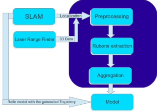
Fig. 1. An overview of our modeling system. 3. SYSTEM DESCRIPTION
The figure 1 presents our method proposed to build a dense representation for an indoor environment, based on 3D planar surfaces. 3D data are acquired via a tilting LRF, and a 2D robot localization is provided by a sparse SLAM process running in background.
Fig. 2. The tilting LRF mounted of the PR2 robot. Data acquired from our tilting LRF (figure 2) is made of a sequence of scan lines. Three pre-processing steps are first executed to prepare data : (1) compute a surfel, i.e. an elementary surface around each point, the area of which depends on its depth with respect to the sensor, (2) manage a circular buffer of three successive lines to create sufficient neighbors around each point; (3) for each point of the middle line, using its neighbors belonging to its elementary surface, compute the normal vector; (4) transform each 3D point in the world frame, and associate each scan line to a robot position to save a link between the SLAM and 3D modeling processes.
The second phase is the plane extraction , which is done using normal vectors and surfels. Let us call a Ribbon, a planar face along a scan line Li, including information from
Li−1 and Li+1 because we cannot theoretically associate
a 3D normal vector from only one scan line:
Ri= {Li−1, Li, Li+1} (1)
Ri is built from the buffer containing three lines L; the
normal vector of Riis computed for the middle line points
Li.
The successive points of Li with close normal vectors
formed a ribbon. A ribbon is extracted in two steps: first points are classified according to the orientation of their normal vectors, then, the classification is refined using the euclidean distance to the origin. Finally a planar represen-tation to the environment is provided from the aggregation of adjacent ribbons in one structure. Each ribbon in the planar structure is associated to its acquisition position
provided by the SLAM process. These positions allow to make consistent our 3D model with the slam process, because the 3D model is corrected as soon as a loop is detected in the SLAM process.
4. DESCRIPTION OF THE MAIN FUNCTIONS 4.1 Preprocessing
Raw data acquired from LRF are points but in spheri-cal coordinates, using ranges and angles (vertispheri-cal tilting angle and horizontal scan angle). First of all, points are expressed with Cartesian coordinates in the robot base frame. The surfel around each point is also created at this level.
Fig. 3. Area estimation for a surfel around a point. The surfel area is computed using the range of each point Piand the vertical and horizontal angular resolutions. The
equation 2 defines this area from these three parameters, shown in figure 3: Si≈ 4ρ2isin( dπ 2 ) sin( dθ 2 ) (2)
ρi is the range of Pi, measured by the LRF. dπ is the
vertical resolution, depending on the tilting velocity. dθ is the horizontal resolution, considered as constant.
Points associated to such a surfel form a subset of the scan line, with a width depending on the depth of Pi. It is
still insufficient to compute a 3D normal vector because all these points are aligned. So we work with one line delay to create a buffer accumulating three successive scan lines. From adjacent surfels on these three lines, we can estimate the normal vector for middle line points. The normal vector is computed using PCA (Principal Component Analysis), using the available function in PCL (Point Cloud Library). From the cartesian coordinates of Piand the normal vector associated to it, we compute the
local plane parameters for the surfel around it, from the equation 3 .
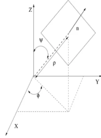
nx.x + ny.y + nz.z + d = 0 (3)
where nx, ny and nz are the normal parameters, d is the
distance to the world origin (origin of the map frame) as shown in figure 4.
The result of the preprocessing step gives a cloud of points, each one defined with its Cartesian coordinates, the parameter of a plane approximating a surfel around it and the surfel area.
Fig. 4. Plane representation
4.2 Ribbons Extraction
Using the data given by the preprocessing step, we classify the points into clusters, gathering neighbor points with close plane parameters.
This clustering function is done in two steps, first classi-fying points according to their normal orientation, then refining the result taking into account the distance from origin. For this reason, we create a 2D grid of 360◦× 180◦,
to cover all possible orientations in the 3D space. In each cell of the grid, we accumulate points with an associated normal close to this orientation. Then, we choose a thresh-old to decide if a group of points represent a plane or not. Because of the variation in the metric resolution of points acquired by a LRF, the number of points observed on a plane change according to the distance of this plane from the range sensor. So, we decided to choose the threshold of detection as an area, and not as a number of points which is used as criterion in most of plane detection algorithms using vote mechanisms.
We put some constrains on the area surface of far points, by giving a smaller value than the one computed in equation 2. The reason is that far points are associated with less accurate normal vectors because of the weak number of neighbours around it. By this way, we prevent far points with large area surfaces and weak normal estimation precision from dominating on other points. It allows to eliminate far points without doing a test at each processing step. We compute the summation of surfels area for points at the same cell, and only points in a cell with a total area greater than a given threshold, are kept as a cluster for the next step.
The information added to a given cluster created from a cell of the grid, are points with their plane parameters, their area surfaces and the existing distances from origin in the form of vector. Durin the second step of the classification, the cluster could be divided in several ones, considering the possible distances to the origin.
As a result for this phase, we had clusters of planes with points grouped in ribbons. In the end, we get a sequence of ribbons representing parts of planes observed from three successive scan lines. This operation is done for each line using the circular buffer of three lines.
4.3 Aggregation
To get a better representation of planar faces located in the explored environment, adjacent ribbons with close parameters have to be merged in the same plane. For this reason, we create a list of planes in the environment. The list will contain potential planes. It has to be empty initially, then add new received ribbons either as a new potential plane or to an existing plane already in the list. New hypothesis is added only if a received ribbon does not belong to any existing planes. To test a ribbon with respect to a potential plane, we test the difference in orientation and in distance. To decide if a ribbon belongs to this plane or not, we compute the probability that this ribbon has the same parameters than this plane. This probability depends on the error on the estimated plane parameters; we assume that the error has a normal distribution with an initial variance Vsensor, and that
it depends only on the measurement error of our range sensor. But other important noise source can influence the quality of estimation, which is the error on the robot localization.
To find the suitable threshold, we tested the quality of estimation of well known plane in the environment in different scenarios. The first case is when the robot is stopped; in this case we can find Vsensor.
In second case, we move the robot in translations and rotations, and estimate the variance Vslam, where the error
of localization impacts also the quality of the estimation. This way we can bound the maximal error, and choose a threshold greater or equal to this error to test ribbons. Let us note here, that the movement done by the robot to find the Vslam parameter, is done only in a local area
around a selected plane, with 3m to 5m translations only, to ensure that the estimation of parameters does not diverge.
Once the thresholds are initialized, we compute the prob-ability of a ribbon to have the same parameters than an existing plane in the list, using a normal distribution of variance Vslam. If the test is positive, we add the ribbon
to the plane.
At this point, the plane structure contains the global parameters of the plane, and all ribbons aggregated to this plane, each one separately with its acquisition position. These positions will serve to rectify the planes parameters, in such a way to keep coherence between our 3D planar model and the SLAM map built during the exploration, and exploited to provide the acquisition positions. The global parameters for a plane are computed using three information which are the local parameters and the areas of each ribbon and their probabilities to be part of this plane.
Nglobal = µ. n
X
i=0
Si.P (Nribbon|Nplane).Nribbon (4)
µ is a normalization factor.
N = {nx, ny, nz, D}T is the normal vector plus the
dis-tance.
P (Nribbon|Nplane) is the probability of a ribbon to belong
to a plane.
The term of Si is added to give more importance to large
ribbons than small ones. 4.4 Model Refining
By now, the more popular SLAM modules are Pose-based SLAM, i.e. SLAM algorithms that use optimization methods to correct the whole trajectory executed by the robot, after a loop closure detection. We tried to exploit such SLAM methods to refine our model. The SLAM process is used during the first steps as a localization tool, allowing to keep all links between the SLAM map and our 3D model; once a loop closure is detected, we take advantage of the optimized trajectory to refine our model. The link we are keeping between the 3D model and the SLAM map, is given by the acquisition positions of every ribbon. We keep this position attached to the 3D data all along the exploration. Once we get a corrected trajectory from the SLAM module, we compute the transformation between the old and the new positions, and apply these corrections to the plane parameters.
To correct the estimated plane parameters, we represent the plane as a 3D oriented point, where the 3D Cartesian coordinates are the product of the distance to the origin by the normal parameters (equation 3), and its orientation is the same as the normal vector:
Pplane= {nx.D, ny.D, nz.D}T (5)
By applying a rotation on the normal vector we correct the normal, then translate the P lane point to get the new distance by normalizing it.
After all corrections are done, we re-aggregate the ribbons together by fusing the ribbons that was detected with different parameters on the same plane.
5. EXPERIMENTS AND RESULTS
Experiments have been done using first the PR2 robot from W illow Garage, and then the Gazebo simulator. All acquisitions have been done in an apartment shown on figure 5, equipped to be used as a realistic indoor environment. All algorithms described in the previous sec-tions have been tested on both actual acquisisec-tions, and simulated ones. Only the model refinement after a loop closure detection, has been validated on the simulator and not on the robot. That is because our currently used SLAM method does not provide a trajectory correction when a loop closure is detected. So we used the simulator to pro-vide a noisy robot localization computed by SLAM module when the 3D model is built, and the true localization without adding any noise when the 3D model is refined after a virtual loop closure.
The SLAM module is the Gmapping SLAM provided as an open source package on ROS. This SLAM module use a 2D occupancy grid to represent the environment as occupied and free zones. It provides also a 2D localization for the robot, at 25 - 30 Hz, in the form of a transform with a rotation expressed as a quaternion. The tilting
Fig. 5. The flat used for our evaluations
LRF provides a 3D point cloud in the form of scan lines, at 40 Hz. To associate each scan line to its localization of acquisition, we need to accelerate the localization fre-quency. This task is done by predicting the localization of robot between two positions provided by SLAM, using the odometer measurements.
Before starting the model construction, some parameters like Vsensorand Vslam, necessary in the next steps, are first
initialized.
5.1 Parameters Tuning
The required parameters are the variances on the angular error and on the distance error for the plane parameters, considering two cases: acquisitions when moving or when stopped. As we have mentioned before in the functions description, we have first chosen a well known plane in the environment, then we computed its parameters with their variance-covariance matrix.
The plane is represented by a normal vector and a dis-tance, the variance of distance is computed directly from distances, and the variance for the normal vectors is com-puted using the scalar product of the normals. These variances can tell us about the error tolerances that will be used after as a condition to fuse a ribbon in a plane. Let us note that the angular and distance tolerances for an acquisition made from a stopped robot, are related directly to the sensor measurement error, i.e. the error in range measured by LRF (about 10 cm), and the horizontal resolution (0.25◦). The tolerances for acquisitions made during motions, depend also on the quality of the SLAM method. If we use only odometry, these tolerances must be greater.
we have tested also the effect of velocity, by using the velocity to rectify scan points during the motion. The results were better with few millimeters only in distance, and about 0.5◦ in angle.
Robot state Angular tolerance Distance tolerance stopped 0.25◦ 10 cm
moving 3.2◦ 25 cm 5.2 Evaluation of our modeling approach
The experiments have been done first using the PR2 robot. The figure 5 shows the flat setting used as a realistic indoor environment to test our approach. The robot has executed
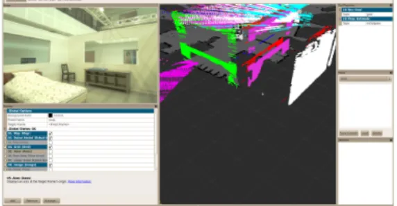
a trajectory around and inside the flat rooms. Inside the flat, we have tested the learning step, where the robot was able to detect the 3D planar faces and build the 3D planar model of the whole environment, as it is shown in figures 6 and 7.
Fig. 6. 3D planes seen from the out side of the room, and the bedroom seen from the robot camera.
Fig. 7. 3D planes detected in the living room(top view), and the living room seen from the robot camera. We have done the same thing with a virtual environment on simulator, where we have built a 3D planar model using the same SLAM module to localize the robot. Then, we used the ground truth path to correct the whole planes estimations after a virtual loop closure. We computed the transformation between the position associated to each ribbon and the corrected position. Then this transforma-tion is applied on each ribbon parameters, by rotating the normal vector and by updating the distance to the origin from the translation.
A long wall which can be observed from several positions in a long trajectory, can especially affected by localization errors. Before the loop closure, they were represented as several small planes with difference in parameters greater than the tolerance on the error threshold. These small planes are corrected ribbon by ribbon, and then, are aggregated in only one larger plane corresponding to the long wall.
Fig. 8. 3D model of the environment: planes in white before correction, in colors after correction.
In figure 8, raw planes are projected on the ground to get a better visualization. In this scenario 110 planes were initially detected; after the SLAM correction, filtering small planes and merging corrected segments, 22 planes are finally extracted after the corrections given by the loop closure detected by the SLAM algorithm.
6. CONCLUSIONS
This paper has presented a method to model a large scale indoor environment. The model is based on planar faces extracted from 3D data acquired from laser range finder on four steps:
• Data acquisition: ranges, transformations and poses. The result of this step is a 3D point cloud expressed in the world frame. 3D points come in the form of sequence of scan lines, not as a matrix. It makes the robot able to move during the acquisition freely without stopping like in the stop and fire strategy.
• Normal estimation and plane detection: we worked with one line delay to create a neighborhood to make the normal estimation possible. The plane detection method is based on the surface estimation of the planar patches, and not the number of points belonging to the plane as in RANSAC algorithms. The proposed method gives a robust estimation of the planar patches around each 3D point, even if they are far away of the robot.
• Ribbons aggregation: all the previous data are processed as scan lines, so the result is expressed as Ribbons that belong to planes. In this step all ribbons that have high probability to belong to the same plane, are listed in one structure; the estimation of the plane parameters are updated each time a new ribbon is detected in the same plane. Finally all points belonging to a same plane are projected on this plane. In order to filter these points, a discrete representation of every plane is built, keeping only on each cell, an occupancy information (this cell has been perceived) and for the perceived cell, the number, the mean and the variance of all points perceived in this cell. • model correction: after a loop closure detected by the SLAM process, a path optimization process will be launched, where the whole path positions will be corrected. At this stage, we have to ensure the consistency of our 3D model with the robot trajectory, applying all the correc-tions propagated along the path.
In our future works we plan to use the detected planes as a basic structure to achieve a high level map by adding semantic information to planes as (wall, door, ceiling and floor) which are the basic identities to build an indoor model (rooms, offices, corridors,. . . ), so that we could jump from labeling objects to labeling topological places. We aim also to add color information to the discrete plane representation to fuse appearance information in our 3D geometrical model.
REFERENCES
A. Aouina, M. Devy, and A. Marin Hernandez. Comparison of Active Sensors for 3D Modeling of Indoor Environments. In Informatics in Control, Automation and Robotics (ICINCO), 10th Int. Conf. on, Reikjavik (Iceland), jul 2013.
B. Douillard, J. Underwood, N. Melkumyan, S. Singh, S. Vasudevan, C. Brunner, and A. Quadros. Hybrid elevation maps: 3D surface models for segmentation. In Intelligent Robots and Systems (IROS), 2010 IEEE/RSJ Int. Conf. on, oct. 2010.
P. Henry, M. Krainin, E. Herbst, X. Ren, and D. Fox. RGB-D Mapping: Using Kinect-Style RGB-Depth Cameras for RGB-Dense 3RGB-D Modeling of Indoor Environments. International Journal of Robotics Research (IJRR), 31(5), April 2012.
A. Hornung, K.M. Wurm, M. Bennewitz, C. Stachniss, and W. Bur-gard. OctoMap: An Efficient Probabilistic 3D Mapping Frame-work Based on Octrees. Autonomous Robots, 2013. Software available at http://octomap.github.com.
B. Huhle, M. Magnusson, W. Strasser, and A.J. Lilienthal. Registra-tion of colored 3D point clouds with a Kernel-based extension to the normal distributions transform. In Robotics and Automation (ICRA), 2008 IEEE Int. Conf. on, 2008.
M. Kaess, A. Ranganathan, and F. Dellaert. ISAM: Fast incre-mental smoothing and mapping with efficient data association. In Robotics and Automation (ICRA), 2007 IEEE Int. Conf. on, 2007.
D. Lee, H. Kim, and H. Myung. GPU-based real-time RGB-D 3D SLAM. In Ubiquitous Robots and Ambient Intelligence (URAI), 2012 9th Int. Conf. on, pages 46–48, 2012.
S. May, D. Droeschel, D. Holz, S. Fuchs, E. Malis, A. N¨uchter, and J. Hertzberg. Three-dimensional mapping with time-of-flight cameras. Journal on Field Robotics, 26(11/12), November 2009. H. Men, B. Gebre, and K. Pochiraju. Color point cloud registration
with 4D ICP algorithm. In Robotics and Automation (ICRA), 2011 IEEE Int. Conf. on, 2011.
R.A. Newcombe, S. Izadi, O. Hilliges, D. Molyneaux, D. Kim, A.J. Davison, P. Kohli, J. Shotton, S. Hodges, and A. Fitzgibbon. KinectFusion: Real-Time Dense Surface Mapping and Tracking. In Mixed and Augmented Reality (ISMAR), IEEE Int. Symp. on, Basel (Switzerland), oct. 2011.
J.I. Nieto, J.E. Guivant, and E.M. Nebot. The HYbrid Metric Maps (HYMMs): a Novel Map Representation for DenseSLAM. In Robotics and Automation (ICRA), 2004 IEEE Int. Conf. on, 2004.
A. N¨uchter and J. Hertzberg. Towards semantic maps for mobile robots. Robotics and Autonomous Systems, 56(11), November 2008.
C. Roussillon, A. Gonzalez, J. Sol`a, J.M. Codol, N. Mansard, S. Lacroix, and M. Devy. RT-SLAM: A Generic and Real-Time Visual SLAM Implementation. Computer Vision Systems, Lecture Notes in Computer Science, 6962, 2011.
R.B. Rusu, Z.C. Marton, N. Blodow, A. Holzbach, and M. Beetz. Model-based and learned semantic object labeling in 3D point cloud maps of kitchen environments. In Intelligent Robots and Systems (IROS), 2009 IEEE/RSJ Int. Conf. on, oct. 2009. R. Smith, M. Self, and P. Cheeseman. Estimating uncertain spatial
relationships in robotics. In Uncertainty in Artificial Intelligence (UAI), 2nd 1986 Annual Conf. on, Corvallis, Oregon, 1986. A. Trevor, J.G. Rogers III, C. Nieto-Granda, and H.I. Christensen.
Tables, Counters, and Shelves: Semantic Mapping of Surfaces in 3D. In Intelligent Robots and Systems, Workshop on Semantic Mapping and Autonomous Knowledge Acquisition (IROS 2010), IEEE/RSJ Int. Conf. on , Taiwan, Oct 2010. IEEE/RSJ. A. Trevor, J.G. Rogers III, and H.I. Christensen. Planar surface
SLAM with 3D and 2D sensors. In Robotics and Automation (ICRA), 2012 IEEE Int. Conf. on, 2012.
T. Tykkala, C. Audras, and A.I. Comport. Direct Iterative Closest Point for real-time visual odometry. In Computer Vision (ICCV Workshops), 2011 IEEE Int. Conf. on, 2011.
J.W. Weingarten and R. Siegwart. EKF-based 3D SLAM for structured environment reconstruction. In Intelligent Robots and Systems (IROS), 2005 IEEE/RSJ Int. Conf. on, 2005.
J. Welle, D. Schulz, T. Bachran, and A.B. Cremers. Optimization techniques for laser-based 3D particle filter SLAM. In Robotics and Automation (ICRA), 2010 IEEE Int. Conf. on, 2010.