Composition sensors calibration and characterization and warmup analysis for the Mars Oxygen In-Situ Resource Utilization Experiment (MOXIE)

(1)

Composition Sensors Calibration and Characterization and

Warmup Analysis for the Mars Oxygen In-Situ Resource

Utilization Experiment (MOXIE)

Presented By

Maya Nasr

B.S. Aerospace Engineering

Massachusetts Institute of Technology, 2018

Submitted to the Department of Aeronautics and Astronautics

as a fulfillment of the requirement for a Master’s Degree in Aeronautics and Astronautics at the

Massachusetts Institute of Technology February 2021

Signature of the Author ___________________________________________________________ Maya Nasr Graduate Student Department of Aeronautics and Astronautics

Signature of Faculty Advisor _______________________________________________________ Jeffrey A. Hoffman Professor of the Practice Department of Aeronautics and Astronautics

(2)

(3)

Composition Sensors Calibration and Characterization and

Warmup Analysis for the Mars Oxygen In-Situ Resource

Utilization Experiment (MOXIE)

Presented By

Maya Nasr

Submitted to the Department of Aeronautics and Astronautics on December 18, 2020 in partial fulfillment of the requirements for the Degree of Master of Science in

Aeronautics and Astronautics

Abstract

MOXIE, the Mars Oxygen In-Situ Resource Utilization Experiment, is one of the payloads that is being carried on the Mars 2020 Perseverance rover. MOXIE was developed by MIT and NASA's Jet Propulsion Laboratory (JPL) to demonstrate, for the first time, In-Situ Resource Utilization (ISRU) on another planet by extracting O₂ from CO₂ in the Martian atmosphere using solid oxide electrolysis (SOE). In order to inform and control its system, MOXIE has a set of temperature, pressure, and composition sensors that measure its internal gas flows. The four composition sensors are commercial off-the-shelf (COTS) hardware and include an oxygen sensor (0 – 100%) and a carbon dioxide sensor (0 – 5%) for the output gas stream from the SOE anode (expected to be pure oxygen) and another carbon dioxide sensor (0 – 100%) and a carbon monoxide sensor (0 – 100%) for the cathode (a mixture of CO2 and CO). Except for the luminescence oxygen sensor, all of these composition sensors are Non-Dispersive Infrared Radiation (NDIR) sensors produced for Earth-ambient-conditions. The research presented in this thesis involves a series of tests under a range of temperatures, pressures and concentrations in order to properly calibrate and characterize (C&C) the sensors to understand their future behaviour on Mars prior to their flight on the Mars 2020 rover. In order to simulate Mars conditions and conduct the C&C tests, this research involved designing and constructing a temperature-controlled vacuum chamber. Following a set test plan, numerous sensor readings were recorded while varying the chamber gas composition, pressure and temperature. The main motivation for this research is to extend the sensor manufacturer’s results, which were designed for operation in stable terrestrial pressure and temperature regimes with frequent calibration, to a Martian environment with large dynamic pressure and temperature swings, variable ratios of gases with cross-sensitivity, and limited ability to calibrate in-situ. This research is critical in characterizing and calibrating the MOXIE sensors prior to their flight on the Mars 2020 rover, in order to be able to correctly interpret their readings.

(4)

Thesis Supervisor: Jeffrey Hoffman

(5)

Acknowledgements

This research would have not been possible without the combined efforts and support from many people. First and foremost, thank you to my advisor, Professor Jeffrey Hoffman, for everything you have done since my very first aerospace engineering class with you during my freshman year of my undergraduate degree at MIT, up until this moment. Thank you for believing in your students and treating us as family. I would not have been able to persevere through some of my most difficult periods at MIT, especially this year, without your genuine kindness, support, and understanding. I am very fortunate to be advised by you.

Thank you to the MOXIE Principal Investigator, Mike Hecht, for your invaluable guidance in this research. Your knowledge and expertise are always inspiring, and I’m looking forward to your continued support during my PhD.

Thank you to the MOXIE team at NASA Jet Propulsion Laboratory (JPL) and outside, particularly to Marianne Gonzalez for your constant help in the sensor LabVIEW VI’s, to Joel Nissen, who never hesitated to generously offer his time and expertise to help in this work, to Asad Aboobaker for your resourcefulness in answering any questions, and to Donald Rapp for your time and patient guidance in the warmup analysis work.

A big thank you to Forrest Meyen for taking me in as a UROP for MOXIE during the end of my sophomore year of my undergraduate degree at MIT. That was one life-changing step in my research path. I am also deeply thankful for Eric Hinterman and my UROP Alex Forsey, both of whom were fundamental parts of this research at every step of the process.

My biggest thank you goes to my family—my wonderful mom and dad, Akhlas and Radwan, and my amazing brother, Samir. You are the main reason I was able to believe in my dreams, leave Lebanon and come to MIT in 2014. Thank you for being there for me at every step of the way, despite the horrific circumstances in Lebanon. You mean more than anything in the world to me, and I wish I were able to be closer to you to celebrate my degree. I owe the three of you everything!

Thank you to all my friends both inside and outside of MIT for making every day fun and memorable and for being always there for me both in every difficult and every happy moment. A special thank you to my best friend, Safa, for being my constant emergency contact and go-to person throughout all my years at MIT.

I would finally like to thank my funding sources. The work in this paper was supported with funding from the MOXIE team supported by three NASA directorates: The Human Exploration and Operations Mission Directorate (HEOMD), the Space Technology Mission Directorate (STMD), and the Science Mission Directorate (SMD).

(6)

List of Figures

Figure 1. Reactions across a SOE cell that extract O2 out of CO2 (Meyen, Hecht, Hoffman, &

Team, 2016) ... 13

Figure 2. Outline of MOXIE subsystems (Meyen, Hecht, Hoffman, & Team, 2016) ... 13

Figure 3. Broken-out view of the MOXIE assembly. Credit: JPL ... 14

Figure 4. Simplified schematic of the MOXIE layout, including the pressure and composition sensors. (Hecht, et al., 2020) ... 15

Figure 5. End–to–end flow diagram for MOXIE showing sensors and transducers (T5 and T6 have been repurposed on the flight model) (Hecht, et al., 2020) ... 15

Figure 6. Absorption Spectra for CO and CO2 (NIST Chemistry WebBook, 2018) ... 20

Figure 7. Design of Sensors Vacuum Chamber (Hinterman, 2018) ... 21

Figure 8. Sensor Vacuum Chamber Internal Design (Hinterman, 2018) ... 21

Figure 9. Sensor vacuum chamber setup with vacuum chamber, pump, and pump controller visible. An inch ruler is added for scale. ... 23

Figure 10. Design of sensors vacuum chamber lid (top down view) (Hinterman, 2018) ... 24

Figure 11. Top view of sensors vacuum chamber lid with both valving manifolds visible ... 24

Figure 12. MOXIE sensor vacuum chamber setup for heating using heat strips ... 25

Figure 13. MOXIE sensor vacuum chamber setup for cooling using fridge ... 26

Figure 14. MOXIE sensor vacuum chamber top view inside fridge ... 27

Figure 15. NDIR Gas Sensor Schematic (NIST Chemistry WebBook, 2018) ... 33

Figure 16. Luminescence quenching in optical oxygen sensors (PreSens Precision Sensing, n.d.) ... 37

Figure 17. CS1 KONZ vs. time plot in 100% CO2 at 20°C ... 40

Figure 19. CS1 Alpha Plot ... 42

Figure 20. CS1 b, n and β0 Plot ... 43

Figure 22. CS1 Pressure Dependence ... 45

Figure 23. CS3 KONZ vs. time plot in 100% CO at 20°C ... 46

Figure 24. CS3 Pressure Dependence ... 47

Figure 25. CS1 KONZ reading vs. Time (CO being added every 90 sec) ... 48

Figure 26. CS1 KONZ reading vs. Time (N2 being added every 90 sec) ... 49

Figure 27. CS1 CO2 density measured vs. total pressure (at CO2 partial pressure = 0.2 bar) ... 49

Figure 28. CS1 CO2 density measured vs. CO or N2 known density ... 50

Figure 29. I0I vs. Pressure for 100% O2 at 70 °C with pressure increments of 0.1, 0.4, 0.7, and 1 bar ... 52

Figure 30. I0I vs. Pressure for 5% CO2 95% O2 at 45 °C with pressure increments of 0.1, 0.4, 0.7, and 1 bar ... 53

Figure 31. I0I vs. Pressure for 5% CO2 95% O2 at 70 °C with pressure increments of 0.1, 0.4, 0.7, and 1 bar ... 53

(8)

Figure 36. MOXIE pressure sensors. P4 measures the cathode exhaust, and P5 measures the oxygen

plenum. (Hecht, et al., 2020) ... 70

Figure 37. MOXIE Flow System Nomenclature. (Hecht, et al., 2020) ... 70

Figure 38. Comparison of Partial Pressure of O2 from CS4, P5 and expected P5. ... 71

Figure 39. CS4 partial pressure and P5 as a function of temperature T15. ... 72

Figure 40. Plots of CS4 partial pressure and P5 Ratio and Difference vs. Temperature T15. ... 72

Figure 41. CS1 and CS3’s KONZ (partial pressure) behavior compared to P4 as a function of time. ... 73

Figure 42. CS1, CS2, and CS3’s KONZ (partial pressure) as a function of temperature. ... 74

Figure 43. Simplified view of SOXE stack. (Hecht, et al., 2020) ... 76

Figure 44. Cutaway schematic showing the physical layout of half of the SOXE. (Hecht, et al., 2020) ... 77

Figure 45. Phase 1 and Phase 2 of warm up cycle. ... 78

Figure 46. The various phase 1 warmup cycles. ... 79

Figure 49. JSA-019 OC5 Stack Temperature during Warmup Phases 1&2. ... 81

Figure 50. Glitches after start in some warm up cycles. ... 82

Figure 51. JSA-019 OC5 Power into SOXE during Warmup Phase 1. ... 84

List of Tables

Table 1. MOXIE NDIR Sensors Modbus Register Overview and Description (smartGAS Mikrosensorik GmbH, 2015) ... 17

Table 2. MOXIE Luminescence Oxygen Sensor Register Overview and Description (PyroScience GmbH) ... 18

Table 3. MOXIE sensor CO2-CO pressure tests at room temperature. ... 29

Table 4. MOXIE sensor CO2-N2 pressure tests at room temperature. ... 30

Table 5. MOXIE cathode sensor temperature tests. ... 31

Table 6. MOXIE anode sensor temperature tests. ... 32

Table 7. ZERO and I0 values for CS1, CS2 and CS3 ... 39

Table 8. Pressure parameter A values for CS1 and CS3 (n=2 fit) ... 47

Table 9. CS1 calibration parameters and assumed conditions in the MOXIE Electrical Interface Control Document Rev G (JPL, 2019) ... 55

Table 10. CS1 calibration parameters with an introduced error of 5% ... 56

Table 11. Legend for Gas Piping Diagram (MOXIE Westford) ... 60

Table 12. MOXIE cathode sensors N2 100% pressure and temperature tests. ... 64

Table 13. MOXIE cathode sensors CO2 100% pressure and temperature tests. ... 64

Table 14. MOXIE cathode sensors CO 100% pressure and temperature tests. ... 65

Table 15. MOXIE cathode sensors CO2-N2 pressure tests at room temperature. ... 65

Table 16. MOXIE cathode sensors CO-N2 pressure tests at room temperature. ... 66

Table 17. MOXIE cathode sensors CO2-CO pressure tests at room temperature. ... 66

Table 18. MOXIE anode sensors N2 100% pressure and temperature tests. ... 67

(9)

Table 21. MOXIE anode sensors CO2-O2 pressure and temperature tests. ... 68 Table 22. Duration of warmup cycles. ... 82 Table 23. Energy dissipated per half-stack in warmup cycles. ... 83

(10)

Chapter 1: Introduction

1.1 Mars Exploration

With its pinkish-red sky, cold, rocky and dry environment, and its waiting-to-be-discovered secrets of past life possibilities, Mars has long been a fascinating planet with a strong appeal for scientists, engineers and humankind overall. Since the 1960’s, the Red Planet has been the target of dozens of exploration missions—flybys, orbiters, landers and rovers—all seeking to understand and answer the questions that humankind has been posing for centuries (Howell, 2019; NASA Science Mars Exploration Program, n.d.).

The idea of life on Mars—whether it existed in the past or not and for future human settlements— has been a discussion spurring worldwide interest since the late 1800’s. It was then when Percival Lowell wrongly saw Martian canals through telescopic observations, raising the possibility of them being built by intelligent beings (Howell, 2012). However, this appeal and curiosity about unleashing the truths of past life on the surface of Mars and about preparing for future human exploration of the Red Planet kept growing over the years, and today it’s stronger than ever.

The list of explorations missions to Mars includes around 49 spacecraft missions. Having successfully made it to Mars are the big players among the space agencies—NASA, the former Soviet Union space program, the European Space Agency and the Indian Space Research Organization (Howell, 2019). China, Japan and other countries, have either tried in the past, or are in the middle of an ongoing launched mission or new mission development. In 1964, Mariner 4 was the first successful flyby spacecraft that sent photos of Mars back to Earth. It was later followed by Mariner 6 and Mariner 7, which showed observations of the craters on the surface of Mars (Howell, 2012). Mariner 9, in 1971, was the succeeding orbiter mission, unveiling the Martian dust storms, dormant volcanoes, and the Valles Marineris canyon (Blasius, Cutts, Guest, & Masursky, 1977).

The next big steps in the history of Martian exploration were the landers followed by the rovers. Viking 1 and Viking 2 were the first two landers that NASA successfully landed on the surface of Mars in 1976. They were followed by the Phoenix lander in 2008. The Viking landers were crucial to characterize and study the Martian atmosphere, image the Martian surface and attempt to search for life. The Phoenix lander made substantial discoveries of frozen water near the surface of Mars while assessing for the local habitability on the planet (Smith, et al., 2009).

NASA’s series of Mars exploration rovers included the Pathfinder lander and Sojourner rover in 1997, Spirit and Opportunity twin rovers in 2004, Curiosity rover in 2012 and most recently the Mars 2020 mission Perseverance rover launched in July 2020. These rovers have contributed some of the most valuable scientific information about the Red Planet and will continue to do. They gave us insight about the past water flow on Mars before it became a frozen desert (Squyres, et al., 2006; Williams, et al., 2013), surface methane detection (Webster, et al., 2015), in addition to organic compounds (Ming, et al., 2014).

The most recent Mars 2020 mission Perseverance rover is the largest, heaviest and most sophisticated NASA rover, and it’s currently on its way to the Red Planet. Perseverance builds on all the knowledge

(11)

18, 2021, Perseverance will look for signs of past microbial life, collect data about Mars’s climate and geology, and will pave the way for future human exploration on Mars. This rover is carrying seven science instruments, including the Mars Oxygen In-Situ Resource Utilization Experiment (MOXIE), which will demonstrate, for the first time, In-Situ Resource Utilization (ISRU) on another planet (Cook, Hautaluoma, & Johnson, 2020).

1.2 Mars In-Situ Resource Utilization (ISRU)

In-Situ Resource Utilization (ISRU) in space missions is the process of using technologies to convert space-based resources at the mission’s destination into needed material and resources, such as propellant, to significantly reduce the cost and risk of carrying the large mass of those resources from Earth. ISRU is often referred to as “living off the land”, and it is crucial for enabling future space exploration missions. Minimizing the launch vehicle mass—which is mostly comprised of the propellant mass—is key, since the initial mass to low Earth orbit (IMLEO) is a first order proxy of the mission’s cost (Drake, 2009).

Ever since the Viking landers confirmed the presence of carbon dioxide (CO2) in the Martian atmosphere in the 1970’s, ISRU technologies on Mars have a been a topic of heavy research (Nier & McElroy, 1997). Making up ~95% of the Martian atmosphere, CO2 is an abundant resource that serves as an excellent candidate for Martian ISRU processes (Muscatello, et al., 2016). The first concepts of Martian ISRU were developed by Ash et al in 1978 in their “Feasibility of rocket propellant production on Mars” study. They proposed a methanation reaction using a combination of atmospheric carbon dioxide CO2 and water to produce methane and oxygen that can be in turn used as a fuel and oxidizer combination for a Mars Ascent Vehicle (Ash, Dowler, & Varsi, 1978). Following that, several methods of ISRU on Mars have been explored over the years, and the importance of these technologies was further highlighted in many reports and mission architecture studies including NASA’s Design Reference Mission 5.0 as a resource to be utilized for ISRU (Drake, 2009).

Some of the ISRU technologies explored and proposed involved CO2 electrolysis, water electrolysis, the reverse water gas shift (RWGS), Sabatier reaction, Bosch reaction, steam reforming, and methane reformation (Sanders, et al., 2015). However, none of these technologies has been yet tested in space— the only technology among them that has been heavily tested on Earth was the Mars ISPP Precursor (MIP) (Sanders & Larson, 2011; Kaplan , et al., 2000). Despite the numerous ISRU-based methane-oxygen propellant ideas, Ramohalli et al.’s manned mission architecture in 1989 initially produced only oxygen on Mars, while carrying methane from Earth, in order to eliminate the complexity of methane production upon landing (Romohalli, Lawton, & Ash, 1989), which would require establishing ice-mining and water purification systems.

The Mars Oxygen In-Situ Resource Utilization Experiment, MOXIE, will be the first demonstration of ISRU in a space mission. It builds upon the notion of using the abundant CO₂in the Martian atmosphere to produce oxygen via solid-oxide electrolysis, according to the process presented in Eq. 1.

(12)

This idea was also put forward by Robert Zubrin in his book, “The Case for Mars”, where he says that all we need to land humans on Mars is, “present-day technology mixed with some nineteenth-century chemical engineering, a dose of common sense, and a little bit of moxie” (Zubrin, 1996). 1.3 MOXIE

MOXIE, the Mars Oxygen In-Situ Resource Utilization Experiment, is one of the payloads that is being carried on NASA’s Mars 2020 rover. It was developed by MIT and NASA's Jet Propulsion Laboratory (JPL) to demonstrate, for the first time, ISRU technologies on another planet (Rapp, Hoffman, Meyen, & Hecht, 2015; Hecht, et al., 2020; Rapp D. , The MOXIE Handbook (Version 118), 2020). MOXIE extracts O2 from CO2 in the Martian atmosphere using solid oxide electrolysis (SOE) (Meyen, Hecht, Hoffman, & Team, 2016). When scaled up in the future, this ISRU-produced oxygen can be used as an oxidizer for the rocket propellants for Mars Ascent Vehicles (MAVs) in human Mars missions, in addition to being used as life support for future Martian astronauts (Nasr, Meyen, & Hoffman, 2018; Hecht, et al., 2020). A MOXIE derived ISRU system can result in large cost and weight reductions for Mars exploration missions, thus making them more feasible and sustainable (Nasr, Meyen, & Hoffman, 2018; Hecht, et al., 2020).

MOXIE is expected to produce at least 6 g/hour of O2 (Rapp, Hoffman, Meyen, & Hecht, 2015). It collects Martian CO2 at a low ambient pressure of ~6 mbar and uses a mechanical pumping system to compress it to roughly 0.7 bar. This compression helps in creating Earth-like operational conditions as the gas is being pumped into the solid oxide electrolysis (SOE) cells shown in Figure 1. (Rapp, Hoffman, Meyen, & Hecht, 2015). Figure 2 shows the three main sub-systems that make up the MOXIE system: Carbon dioxide Acquisition and Compression (CAC), Solid Oxide Electrolysis (SOE), and Monitor and Control System (MCS). Figure 3 is a broken-out view of the MOXIE assembly, showing the compressor on the far left, the SOXE assembly and sensor panel in the center, and the closed-up MOXIE on the right.

On this sensor panel, MOXIE has a set of temperature, pressure and gas composition sensors. There are four commercial off-the-shelf (COTS) composition sensors, three of which are Non-Dispersive Infrared Radiation (NDIR) sensors measuring carbon dioxide on the cathode and anode sides and carbon monoxide at the cathode. The fourth sensor is a luminescence oxygen sensor at the anode side. These four composition sensors are produced for Earth-ambient conditions and thus must be calibrated to understand their behavior under Mars-like conditions. The research in this thesis focuses on the calibration and characterization of the four gas composition sensors under a range of temperatures, pressures and concentrations in order to understand their future behavior on Mars.

(13)

Figure 1. Reactions across a SOE cell that extract O2 out of CO2 (Meyen, Hecht, Hoffman, & Team, 2016)

(14)

(15)

Chapter 2: Materials and Methods

2.1 MOXIE Gas Composition Sensors

MOXIE has a set of sensors to track its temperature and pressure and to track the flowing gas composition in order to inform its behavior. These sensors are shown in Figure 4. Figure 5. End–to– end flow diagram for MOXIE showing sensors and transducers (T5 and T6 have been repurposed on the flight model) .

Figure 4. Simplified schematic of the MOXIE layout, including the pressure and composition sensors. (Hecht, et al., 2020)

(16)

MOXIE has four commercial off-the-shelf (COTS) composition sensors. These four sensors are represented in Figure 5 and throughout this paper as CS1, CS2, CS3, and CS4, corresponding to the cathode carbon dioxide sensor, the anode carbon dioxide sensor, the cathode carbon monoxide sensor and the anode oxygen sensor respectively. All of these composition sensors except the luminescence oxygen sensor are Non-Dispersive Infrared Radiation (NDIR) sensors produced by the smartGAS company located in Germany. These NDIR sensors measure the attenuation of an infrared beam passing through the gas volume by comparing a reference and a measured intensity from the non-absorbing and non-absorbing (target gas) channels respectively. Its internal algorithms use the Beer-Lambert law to normalize and linearize the ratio of outputs from the detector against the reference. These algorithms also correct for temperature dependency and then determine the final partial pressure of the gas using the ideal gas law relative to a hypothetical 1 bar atmosphere (Hecht, et al., 2020; smartGAS Mikrosensorik GmbH, 2015). The oxygen sensor, from PyroScience company located in Germany, measures the O2 partial pressure with an intrinsic accuracy of ±2% full–scale (0.012 bar) (PyroScience GmbH; Hecht, et al., 2020). It is important to note that all of the sensor measurements are redundant and could be verified in comparison to gas composition calculations using temperature and pressure sensors, in addition to motor speed and SOXE current.

The IR radiation from the source interacts with the gas as it passes in the optical cavity on its way to hit the dual channel detector, which consists of an active and a reference channel. The active channel exclusively allows the wavelength of an absorption band to pass through its filter while the reference channel, on the contrary, allows the rest of the no-absorption-band wavelengths to pass.

The SOE anode is expected to be pure oxygen, except for any potential CO2 and CO leaks that occur and pass through to the anode. However, any CO that leaks to the anode will immediately recombine with an oxygen ion and become a CO2 molecule. From here, in addition to the CS4 oxygen sensor on the anode side, the CS2 carbon dioxide sensor is sufficient to detect any leaks and to verify the purity of the output oxygen stream. Because only a small amount of CO2 would be present in the anode in the case of a leak, the CS2 carbon dioxide sensor has a range of 0–50 mbar pCO2 at room temperature,

with a stated accuracy of ±2% of full–scale (Hecht, et al., 2020; smartGAS Mikrosensorik GmbH, 2015).

On the SOE cathode side, however, a different behavior is expected, dictated by both the utilization rate of CO2 set by the MOXIE team and by the voltage changes in the SOE stack. Although the inlet of the cathode stream will be mostly CO2, the amount of CO2 that will react with the electrolyte to produce CO and O2- will vary with the previous said factors, causing a variance in the expected content of the stream. From here, in addition to the CS1 carbon dioxide sensor on the cathode side, the CS3 carbon monoxide sensor is used. Both the CS1 carbon dioxide sensor and CS3 carbon monoxide sensor have a range of 0–1000 mbar (assuming room temperature), with a stated accuracy of ±8% full–scale (Hecht, et al., 2020; smartGAS Mikrosensorik GmbH, 2015).

MOXIE’s three NDIR sensors, CS1, CS2 and CS3, each have 13 data registers. These registers and their corresponding descriptions can be seen in Table 1 below. For the purposes of this research, several LabVIEW Visual Instruments (VI’s) were developed in order to read and save the data from these registers. The main focus was on the first 16 registers, in addition to the SPAN and IR_4tagneu (ZERO) registers. As mentioned previously, the challenge is to use the individual register readings to understand how the proprietary algorithms that govern the sensor composition readings depend on

(17)

Table 1. MOXIE NDIR Sensors Modbus Register Overview and Description (smartGAS Mikrosensorik GmbH, 2015)

Reg.-No. Name Description

1 0x00 IR_m_pre IR intensity signal from the measurement channel 2 0x01 Ref_m IR intensity signal from the reference channel

The IR-source is regulated onto Ref_m Occuring changes of Ref_m could be noticed

indirectly by a change of I_Str

3 0x02 IR_m Relation between measurement and reference

channel

4 0x03 T_m relative sensor temperature x 0.1°C (not absolute!) 5 0x04 IR_korr IR_m signal temperature corrected at zero 6 0x05 MOD Modulation - non linearized concentration signal

7 0x06

8 0x07

9 0x08 IR_4tag floating average of IR_korr over 96h

10 0x09 Sys_status Status bits

Bit 00 TEST_FLAG 1 = self test running after power on

Bit 01 WARMUP_FLAG 1 = warming up after power on

Bit 02 SYSERR_FLAG 1 = system error --> see table below

Bit 05 STARTUP_FLAG 1= start up Bit 12 EEP_ERROR 1 = EEPROM error

Bit 13 WDG_WARN 1 = watchdog error Bit 14 POWER_ON 1 = power suplly connected

11 0x0A Konz Gas concentration signal

12 0x0B MOD_korr Modulation corrected by temperature

13 0x0C I_str Supply current for the IR source x 0.01 mA

14 0x0D Num_Ein Buffer for number of power on

0x0E Num_4h Operating time (multiple of 4 hours)

0x0F

0x10+ Protected, do not cross with multi-register command

0x47 IR_4tagneu Zero

0x4F Unit Unit (%vol, ppm, or %UEG): 4 = CS2 x 0.001 or 5 = CS1 & CS3 x 0.01

(18)

0x85 SW Software Version

0x86 SN Serial Number

0xC0 Address Modbus Address

MOXIE’s fiber optic luminescence oxygen sensor, CS4, has 13 data registers, which are described in Table 2 below. The first 8 registers (addresses 0-7) contain the most essential data, according to the manufacturer. The fundamental raw data of the oxygen measurement is the “phase shift” dphi. The CS4 oxygen sensor then uses the Settings registers and the Calibration registers to convert dphi into oxygen units of “mbar” and “%O2” in the mbar and percentO2 registers (PyroScience GmbH). It is important to note that the “%O2” units are provided only for convenience and under the assumption of 1013 mbar ambient gas pressure. The way the CS4 oxygen sensor calculates this percentage value is by using the measurement of the internal pressure sensor to convert the oxygen partial pressure into units of %O2, only “if the air pressure at the oxygen sensing membrane is identical to the air pressure at the venting capillary on the backside of the housing” (PyroScience GmbH). For the purposes of this research, FireDiskO2 Logger v134 software was used in order to read and save the data from these registers (PyroScience GmbH).

Table 2. MOXIE Luminescence Oxygen Sensor Register Overview and Description (PyroScience GmbH)

Address Label Unit Range Default Description

1 0 status 0-256 0 Status byte with bit0: reserved,

bit1: sensor signal too low, bit2: sensor signal or background light too high, bit3: reference signal too low, bit4: reference signal too high, bit5: no external temperature sensor detected, bit6: init flag (=0 after power up, set to 1 as a flag in order to detect power cycling)

2 1 dphi mo _±231 ₀ _{Phase shift of oxygen}

measurement (raw data)

3 2 umolar nmol/L ±231 0 Oxygen level in units of µmol/L (valid only in liquids)

4 3 mbar _µbar _±231 ₀ _{Oxygen level in units of mbar}

5 4 airSat 10-3 %air

sat. ±231 0 Oxygen level in units of % air saturation (valid only in liquids)

6 5 tempSample m°C ±231 0 Sample temperature

7 6 tempCase m°C ±231 0 Case temperature

8 7 signalIntensity _µV _±231 ₀ _{Signal intensity of oxygen} measurement (peak-peak)

(19)

9 8 ambientLight _µV _±231 ₀ _{Ambient light measured just} before oxygen measurement 10 9 pressure µbar ±231 0 Ambient air pressure (not

implemented)

11 10 humidity m%RH ±231 0 Relative humidity (not implemented)

12 11 resistorTemp mOhm

(µV) ±231 0 Resistance of the temperature sensor (analog input) 13 12 percentO2 m%O2 ±231 0 Oxygen level in units of %O2 2.2 Characterization and Calibration (C&C)

Sensor calibration and characterization is critical to the MOXIE team, as the results dictate the interpretation of the MOXIE composition sensor readings on Mars. Since these sensors were originally designed for operating in Earth-ambient conditions, there are no prior expectations of their behavior under Martian pressure and temperature conditions. Therefore, it is important to conduct C&C testing of these MOXIE compositions sensors under Mars-like conditions to understand their pressure and temperature dependence. Additionally, the tests will give a better insight into the sensors’ response time to changes in gas concentration, as well as giving a better understanding of their aging and degradation over time—an understanding of great importance, especially for future long-duration missions.

Another motive for the calibration and characterization tests is to measure the cross-sensitivity that occurs between gases, as measured by the sensors. Since the three CO2 and CO composition sensors of interest in this research—CS1, CS2, and CS3 —are all NDIR sensors, their readings of gas composition are determined by the quantity of light absorbed over a certain frequency range. This raises the potential problem of cross-talk or cross-sensitivity in the sensor readings between two gases due to the potential overlap in the CO2 and CO IR absorption spectrum, as shown in Figure 6. In the shaded region of overlapping spectra, the CO sensor could mistakenly detect CO2 as CO gas, and the CO2 sensor could mistakenly detect CO as CO2 gas. Thus, it is crucial to understand and quantify this cross-sensitivity in order to correctly account for its effect on the sensors’ readings during their operation. Testing the cross-sensitivity involves a set of tests where both sensors are placed in a 100% CO2 filled chamber, then in a 100% CO filled chamber, and finally in a chamber filled with a pre-known mixture of both gases. In each of these conditions, a set of tests at different pressures was conducted. Furthermore, cross-sensitivity is also identified and tested by comparing measurements of a CO2/CO gas mixture to a CO2/N2 mixture and quantifying the difference between the measurements.

(20)

Figure 6. Absorption Spectra for CO and CO2 (NIST Chemistry WebBook, 2018)

Targeting measuring properties that vary between units, calibration tests will calibrate the sensors’ “ZERO Offset” at 0% of the target gas and “SPAN” at 100% (or 5% for CS2) of the target gas at a range of pressures and temperatures. Additionally, during flight operations, after MOXIE startup in every run, a single point in situ calibration against the Mars ambient atmosphere will be performed using pressure and temperature measurements from the Mars Environmental Dynamics Analyzer (MEDA) instrument on the Perseverance rover.

In contrast to the calibration, the characterization measurements focus mainly on the general behavior and properties of the system and will help in determining the previously discussed cross-sensitivity dependence in the sensors’ readings.

2.3 Vacuum Chamber at MIT

In order to simulate the Martian conditions for the purposes of the calibration and characterization test environments, it was necessary to design and build a temperature and pressure controlled vacuum chamber to house the sensors during the experiments. The design of this small vacuum chamber can be seen in Figure 7 below, with its side view and internal design shown in Figure 8.

Mars 2020 Project

The technical data in this document are controlled under the U.S. Export Regulations. Release to foreign persons may require an export authorization Pre-Decisional: For Planning and Discussion Purposes Only.

CO

₂

/CO Mixture Spectral Overlap

12

CO

₂

CO

The SmartGas CO2sensor is

insensitive to the presence of CO

The SmartGas CO sensor is very sensitive to the presence of CO2 http://webbook.nist.gov/chemistry O ve rla p of sp ect ra

(21)

Figure 7. Design of Sensors Vacuum Chamber (Hinterman, 2018)

CO2

Regulator Needle Valve Flow Meter

N2

Regulator Needle Valve Flow Meter

Manifold Ball Valve Vacuum Chamber Oven or Ice Cooler Small Pump Vacuum Pump To Vent Bypass for Purging Pump Controller

MOXIE Sensors Vacuum Chamber

Created by Eric Hinterman Modified Feb 7, 2018

Sensor

Ball Valve

(22)

This setup operates by flowing gas from pressurized CO2, N2, and CO gas tanks to the central manifold through a series of regulators and ball valves before it passes through the sensors and the vacuum pump, to be finally vented out into an exhaust hood in the lab. The ball valve immediately after the manifold was used to isolate the chamber after the chamber has been filled with a certain pressure of gas. A small pump was used for recirculating the gas throughout the chamber to provide better flow through the sensors. Additionally, as shown in Figure 8, the gas sensors were used in a flow-through rather than static approach. The reason behind this approach, which involves attaching a tube to the sensors’ outlets into the recirculation line, is to force the gas to be pulled through the sensors to ensure better flow and thus more accurate SmartGas sensor readings.

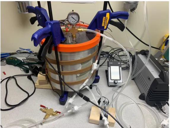
Figure 9 shows the actual set up, consisting of the vacuum chamber, the pump controller, and the vacuum pump, in order from left to right, with 1/4” inner diameter and 3/8” inner diameter Tygon tubing to connect the system together. Figure 10 and Figure 11 show the schematic design of the chamber lid and its real top view, respectively. As portrayed in these two figures, the chamber lid consists of two pre-drilled holes, to which two manifolds were attached. These manifolds accommodated five paths into or out of the chamber: the gas inlet line, the pressure gauge (“P” in Figure 10), an unused port, the gas outlet line, and an air filter. The main purposes of these connected paths were to allow the gas to flow from the gas cylinders or recirculation loop through the gas inlet and out to the recirculation loop or exhaust hood through the gas outlet. Additionally, the pressure gauge was used to measure the level of vacuum in the chamber, and the filter to prevent the entry of any dust particles when re-pressurizing the chamber with ambient air.

From here, it is easy to obtain a needed gas composition in the chamber by adding the specific amounts of each desired gas into the chamber sequentially. The relative amounts are monitored by the total pressure in the chamber. The chamber was always evacuated to near-vacuum at the beginning of each run, then filled sequentially with the amount of each desired gas independently. The recirculation pump helped in cycling the air and ensuring the gases in the chamber mixed properly.

In order to power the system and to receive the sensor’s data readings on the computer, it was necessary to have a minimum of 7 cables passing through the chamber lid. This was a challenge due to the importance of avoiding any potential leaks to the chamber through these cables. In order to install these electrical feedthroughs, 18-gauge copper wire pieces were inserted into a set of 1/4” holes drilled in the chamber lid. Power and USB cables were stripped and connected to the copper wire pieces. Vacuum epoxy was used to fill each of the holes around the wire, preventing any potential leaks in the system.

(23)

Figure 9. Sensor vacuum chamber setup with vacuum chamber, pump, and pump controller visible. An inch ruler is added for scale.

(24)

Figure 10. Design of sensors vacuum chamber lid (top down view) (Hinterman, 2018)

(25)

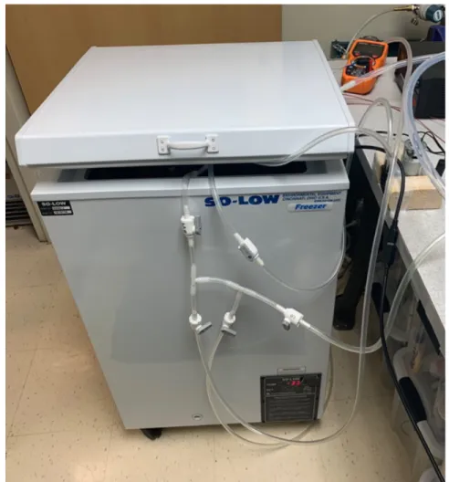
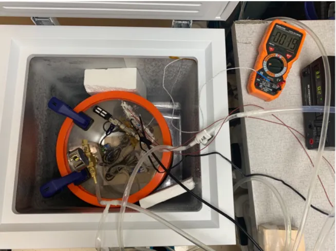
In order to control the vacuum chamber’s temperature, the chamber was heated using heat strips that were wrapped around it, as seen in Figure 12. In order to achieve cold temperatures, the chamber was placed in a small freezer as shown in Figure 13 and Figure 14. These systems were tested and proved effective at maintaining the required range of temperatures for the C&C tests.

(26)

(27)

Figure 14. MOXIE sensor vacuum chamber top view inside fridge

2.4 MIT Experimental Testing Plan

The first step in this research was creating a standard operating procedure (SOP) that was approved by the MIT MOXIE Team. Approval from MIT Environmental Health and Safety personnel was also required to ensure that no poisonous or flammable gas mixtures would be generated. Next, a set of tests following an agreed-upon test plan was conducted. These calibration and characterization (C&C) tests involved the four sensors CS1, CS2, CS3 and CS4.

The test plan was designed to test the sensor readings at a range of varied chamber parameters: gas composition, temperature and pressure. Being designed for Earth-ambient operating conditions (at atmospheric pressure ~1 bar), it is important to understand the effect of Martian temperatures and pressures on the sensors’ readings. Although MOXIE will run internally at roughly 0.7 bar, it is important to test the sensor’s behavior at pressures that range from as low as the Martian ambient pressure (~0.005 bar), which will be expected at the start of MOXIE runs, all the way up 1 bar. From here, the set of tests targeted a range of pressures from near 0.005 bar (limited by the vacuum

(28)

they measure the outside air after it has passed into the rover and warmed up a bit. Additionally, the test plan included a range of known gas concentrations that were altered throughout the range of pressures and temperatures to understand the effects of cross-talk between gases.

This experimental test plan is shown in Table 3, Table 4, Table 5, and Table 6 below. Table 3 shows the 44 MOXIE sensor CO2-CO pressure tests that were conducted with a range of different gas compositions at room temperature. Table 4 shows the remaining 24 CO2-N2 pressure tests that were conducted at room temperature. Table 5 shows the 32 MOXIE cathode sensor temperature tests that were conducted at a range of -30 degrees Celsius to 70 degrees Celsius. It is important to note that throughout all those tests in Table 3, Table 4, and Table 5, only the CS1 and CS3 sensors were placed in the chamber. Table 6 shows the 49 MOXIE anode sensor temperature tests that were conducted at a range of -30 degrees Celsius to 70 degrees Celsius at a range of concentrations and pressures. During the tests in Table 6, only the CS2 and CS4 sensors were placed in the chamber. Additionally, throughout the test runs, a 90-second wait period was implemented between each of the tests that were conducted at room temperature, and a 10-minute wait period was implemented between each of the tests that were conducted at high or low temperatures to ensure that the added gas to the chamber reached the desired temperature after each addition.

All of the sensors were connected to a computer, where the readings from the first 16 of the NDIR sensor registers (see Table 1), in addition to the 0x54 SPAN and the IR_4tagneu ZERO registers, were recorded and saved using several LabVIEW VI’s. The readings from the luminescence oxygen sensor register (see Table 2) were saved using FireDiskO2 Logger v134 software. These recorded readings were used in a series of analyses and equations that will be discussed later in this paper.

(29)

(30)

(31)

(32)

(33)

Chapter 3: Theory and Calculations

3.1 The Beer-Lambert Law for Gas Absorption

One unique property of certain gas molecules is their ability to absorb infrared (IR) radiation. If the gas’s wavelength matches the natural frequency of the molecule, IR radiation can change the energy state of the molecule’s atoms, thus increasing their chemical bond vibrations. However, this molecule-radiation interaction requires the presence of a dipole in the molecule — something that makes molecules like those of carbon dioxide (CO2) and carbon monoxide (CO) good candidates for this phenomenon (SGX Sensortech (IS) Ltd, 2007).

This infrared gas absorption property can be used in several applications, including gas sensors. There are two types of gas sensors used: Dispersive Infrared and Non- Dispersive Infrared (NDIR).

Dispersive Infrared instruments are generally a large and expensive type of gas spectrometer used in laboratories. These instruments use the diffraction of the IR passing through them before the dispersed spectrum crosses to a detector (SGX Sensortech (IS) Ltd, 2007). Non-Dispersive Infrared (NDIR) sensors, on the other hand, normally consist of an IR source, followed by an optical cavity, then an IR active and an IR reference detector (Alphasense, 2014).

Figure 15. NDIR Gas Sensor Schematic (NIST Chemistry WebBook, 2018)

The IR radiation from the source interacts with the gas as it passes in the optical cavity on its way to hit the dual channel detector, which consists of an active and a reference channel. The presence of these two separate channels is important throughout the process. The active channel exclusively allows

(34)

importance of performing calibration and characterization (C&C) tests to properly account for these effects.

NDIR sensor readings are generally governed by the Beer-Lambert law for gas absorption. The decrease in the IR gas intensity in the active channel detector is governed by the Beer-Lambert law exponential in Eq. 2 below. It is important to note that the NDIR sensors cannot measure the volume percent “concentration”—they are very dependent on the number of molecules (and thus the gas density) rather than the percentage volume.

𝐼 = 𝐼₇𝑒9(;<=) Eq. 2

Where I is the intensity in target gas, 𝐼7 is the intensity in zero target gas, K is a factor accounting for the filter and the gas absorption lines [L mol-1_cm-1_{], L is the optical path-length between the IR source} and the detectors [cm], and C is the concentration (molar density) of the gas [mol L-1_{] (SGX Sensortech} (IS) Ltd, 2007). Additionally, the corresponding voltage drop in the active detector is according to Eq. 3 (SGX Sensortech (IS) Ltd, 2007).

(𝑉7− 𝑉) 𝑉₇ =

(𝐼7− 𝐼)

𝐼₇ Eq. 3

Where V and I are the respective output voltage and current in target gas, and 𝑉7 and 𝐼7 are the respective output voltage and current in zero gas (SGX Sensortech (IS) Ltd, 2007).

Combining Eq. 2 and Eq. 3 helps in measuring the (@A9@)

@A term known as the Fractional Absorbance (FA) in the sensor as shown in Eq. 4. The value of FA increases with the concentration (molar density) C, but is affected by the values of K and L.

𝐹𝐴 = 1 − 𝑒9(;<=) Eq. 4

However, this Beer-Lambert law calculation is very idealistic. It does not take into account a multitude of factors, including the variation of filter band passes, spectral output changes, and the effects of pressure and temperature on the reading. A more realistic approach to understanding the readings of NDIR sensors is using the Modified Beer-Lambert Law shown in Eq. 5. This version introduces additional coefficients, a and n, to account for these effects.

𝐼 = 𝐼₇𝑒9(E=F) Eq. 5

The effects vary with the target gas and sensor, as shown in Eq. 6.

𝑁𝐴 = 1 − 𝐼

𝑍×𝐼₇ Eq. 6

Where the reference detector ratio is accounted for in the term 𝑍 =_JJ A=

@KLM @_KLMA.

(35)

𝑁𝐴 = 1 − (_@@ A)( @_KLMA @KLM )= 1 − ( N NKLM) ( NA NKLMA) = 1 − (_JJ A) Eq. 7

Finally, combining Eq. 2 and Eq. 7 with an introduction of a “SPAN” factor can be used as a method of calculating the gas concentration C, according to Eq. 8. (SGX Sensortech (IS) Ltd, 2007).

1 − J

JA = 𝑆𝑃𝐴𝑁 ×(1 − 𝑒

9(E=F)₎ Eq. 8

Where SPAN is the fraction of the IR radiation on the active detector that has the ability to be

absorbed by the target gas—it is the end point reference value (Alphasense, 2014; smartGAS Mikrosensorik GmbH, 2015).

However as mentioned before, this reading is sensitive to effects of pressure and temperature. These effects can normally be accounted for using the ideal gas law, as shown in Eq. 9. However, any additional effects that temperature and pressure introduce in the components of the NDIR sensing system have to be separately accounted for outside of the ideal gas law equation (SGX Sensortech (IS) Ltd, 2007).

𝐶 = 𝑘 𝑃@_R Eq. 9

Where 𝑘 is a constant, P is the gas pressure, V is the gas volume and T is the gas temperature in Kelvin.

Thus, it is very important to calibrate the sensors to account for these temperature and pressure effects. This calibration to properly calculate the gas concentration is dictated by understanding the sensor’s absorbance (ABS), in addition to the ZERO and SPAN parameters as defined in Eq. 10, Eq. 11, Eq. 12, and Eq. 13 below (Alphasense, 2014).

𝐼₇ is the ratio of the active signal 𝐴𝐶𝑇7 to reference signal 𝑅𝐸𝐹7 when there is no target gas present (zero gas setting).

𝐼₇ = 𝐴𝐶𝑇7 𝑅𝐸𝐹₇ = 𝑍𝐸𝑅𝑂 Eq. 10 Absorbance: 𝐴𝐵𝑆 = 1 − (_JJ A) Eq. 11 𝑆𝑃𝐴𝑁 = WXYZ [9+\(]Z^) Eq. 12 𝐴𝐵𝑆_{_} = 𝑆𝑃𝐴𝑁(1 − 𝑒9 `_^ ₎ _{Eq. 13}

(36)

From here, the absorbance ABS can be calculated and used to find the concentration (molar density) of the gas ′x′ according to Eq. 14 assuming positive absorbance (Alphasense, 2014).

x = [ln 1 − 𝐴𝐵𝑆𝑆𝑃𝐴𝑁

−𝑏 ](

[

-) Eq. 14

Where ABS is the absorbance, SPAN is the proportion of absorbing radiation (determined during calibration), and b and c are the linearization coefficients from Eq. 13 (Alphasense, 2014).

In order to correct for the effect of temperature on the absorbance (ABS), SPAN, and the gas concentration, additional correction coefficients must be introduced to the previous calculations, as shown in Eq. 15, Eq. 16, Eq. 17, and Eq. 18 below (Alphasense, 2014). These equations assume a linear dependence on temperature (which is observed in the experimental results presented in Chapters 4 and 5).

𝑆𝑃𝐴𝑁_R = 𝑆𝑃𝐴𝑁_-E,+ 𝛽₇ 𝑇 − 𝑇_-E, Eq. 15

(1 − 𝐴𝐵𝑆_R) = (1 − 𝐴𝐵𝑆)(1 + 𝛼 𝑇 − 𝑇_-E, ) Eq. 16

𝑆𝑃𝐴𝑁_R = 𝑆𝑃𝐴𝑁_-E,+ 𝛽_W 𝑇 − 𝑇_-E, Eq. 17

Where 𝑆𝑃𝐴𝑁R is the SPAN corrected at temperature T, 𝛽7 is the temperature correction coefficient of only SPAN, 𝐴𝐵𝑆_𝑇 is the temperature corrected absorbance at temperature T, 𝛼 is the absorbance temperature correction coefficient, and 𝛽W is the ABS and SPAN temperature correction coefficient. The intensity correction can thus be written as:

𝐼(R) = 1 + 𝛼 𝑇 − 𝑇-E, ×𝐼-E, Eq. 18

It is important to note that for the purpose of the MOXIE NDIR sensors, the manufacturer recommended that we never adjust the values of SPAN and ZERO in the sensor’s firmware, since that is done at the factory (at STP). The sensors do their own temperature correction, but it is recommended that temperature calibrations be done and pressure calibrations if the pressure deviates from 1 atm.

Finally, the ideal gas law can be employed in order to calculate the final gas concentration (molar density) at temperature T as shown in Eq. 19 (Alphasense, 2014).

x = 𝑇 𝑇_-E, { ln 1 − 𝐴𝐵𝑆R 𝑆𝑃𝐴𝑁R −𝑏 [ -} Eq. 19

(37)

3.2 Oxygen Luminescent Sensing

Oxygen luminescent sensing is based on the mechanism of quenching by molecular oxygen, as oxygen is one of the most powerful luminescence quenchers (Borisova, 2018; Jiang, Yu, Zhai, & Hao, 2017; Rusak, James, III, Ferzola, & Stefanski, 2006). As pictured in Figure 1, this process starts by an LED light exciting the optical oxygen sensor (the indicator) to emit fluorescence whose intensity, decay time and wavelength are dependent on the oxygen partial pressure (Jiang, Yu, Zhai, & Hao, 2017; PreSens Precision Sensing, n.d.). If a collision with oxygen molecules happens, the fluorescence signal gets “quenched”. In other words, the excess energy from the excited state gets a non-radiative transfer to the oxygen molecule, thus decreasing the signal. This quenching measurement is a direct indicator of the partial pressure of oxygen present, and the decay time is measured internally (PreSens Precision Sensing, n.d.).

Figure 16. Luminescence quenching in optical oxygen sensors (PreSens Precision Sensing, n.d.)

It is important to be able to quantify the fluorescence lifetime—the decay time needed for the fluorescence intensity to decay to 1/e of its initial value after an excitation. Since fluorescence lifetime is reduced with quenching, one can use the lifetime values to measure collision rates in the process and can gather information about temperature, polarity, etc. The fluorescence lifetimes can be quantified using the slope of plots of natural log of fluorescence intensity versus time (Rusak, James, III, Ferzola, & Stefanski, 2006).

(38)

Where 𝜏 is the luminesce lifetime and 𝐼 is the luminesce intensity, both at a certain concentration of O2, and 𝜏7 is the luminesce lifetime and 𝐼7 is the luminesce intensity, both in free condition (in the absence of a quencher). 𝑘_m is the bimolecular quenching constant (determined mostly by oxygen diffusion) and 𝐾2o is the Stern–Volmer constant (Jiang, Yu, Zhai, & Hao, 2017; Borisova, 2018). The Stern–Volmer quenching plots (pA

p or JA

J vs 𝑂( ) are valuable tools to analyze the luminesce lifetime and quenching rate constants (Rusak, James, III, Ferzola, & Stefanski, 2006; Payne, Fiore, Fraser, & Demas, 2010). A plot of J_JA vs. partial pressure of O2 produces a straight-line relationship that helps quantifying the value of 𝐾2o. This linearity could be observed in a homogenous medium, and it indicates that only one type of quenching (a collisional quenching mechanism) occurs (Topal, Ertekin, Topkaya, Alp, & Yenigul, 2008)

However, since the process of luminesce/fluorescence quenching is dependent on the rate of collisions, temperature can have strong impact on the results, as it determines the force imparted by each collision. Cross-sensitivity to temperature can affect the phosphorescence decay time, causing faster oxygen diffusion and hence a decrease in 𝜏7, in addition to an increase in the Stern–Volmer constant for the same reasons (Borisova, 2018). Hence, it’s important to calibrate the measured plots relating luminescence intensity to partial pressure at different temperatures in order to correct of this effect. A two-point recalibration for the Stern-Volmer plot with an additional temperature measurement could resolve the problem, but it’s important to note that the gas phase, temperature, atmospheric pressure and relative humidity should be measured during calibration (Borisova, 2018).

(39)

Chapter 4: Results

4.1 Experimental Tests at MIT

4.1.1 CS1, CS2 and CS3

In order to analyze the set of data that was recorded from the experiments, several steps were involved. Firstly, using the 0x0054 SPAN and the IR_4tagneu ZERO registers, the values of SPAN and ZERO for each of the sensors were recorded. Additionally the values of 𝐼₇ for each of the sensors was calculated. It’s important to note that 𝐼₇ = Jq_s_t/+_q+u

v when there is no target gas present, where using Table 1, 𝐼𝑅_𝑚_𝑝𝑟𝑒 is IR Intensity signal from the measurement channel and 𝑅𝑒𝑓_s is IR intensity signal from the reference channel. The value of 𝐼7 is a calibration step done once at the beginning of each test. This value can be calculated by either finding the value of Jq_s_t/+_q+u

v taken in zero target gas (in 100% Nitrogen) or by calculating 𝐼₇ = {|_}~•€•‚ƒ_[7777 . This research used the latter equation in calculations. The SPAN, ZERO and 𝐼7 values for the three sensors CS1, CS2 and CS3 are shown in Table 7 below.

Table 7. ZERO and 𝐼₇ values for CS1, CS2 and CS3 SPAN ZERO 𝐼₇

CS1 10000 17164 1.7164 CS2 10000 7491 0.7491 CS3 10000 11585 1.1585

These NDIR sensors use the “0x0054 SPAN” register which has a correction value in order to determine the end point and internally evaluate the gas composition. The value of SPAN is preset to 10, 000 by the smartGAS company. After this scaling, the composition information is presented as a volume percent reading in the 0x000A KONZ register. However, in order to correctly read the composition in the 0x000A KONZ register, the 0x004F Unit register must be used. For MOXIE purposes, the value of 0x004F Unit register is 4 for CS2 and 5 for CS1 and CS3. Thus according to the smartGAS sensor manual, the KONZ1 and KONZ3 readings of the CS1 and CS3 sensor should be multiplied by 0.01, and the KONZ2 of the CS2 sensor should be multiplied by 0.001 (smartGAS Mikrosensorik GmbH, 2015). This percent volume concentration reading would be interpreted assuming pressure of 1 bar and ambient temperature.

Figure 17 and Figure 18 show an example of the KONZ reading for the CS1 sensor (multiplied by 0.01). Figure 17 shows a series of 100% CO₂ tests where the CO₂pressure was increased from 0.005 bar up to around 1 bar by 0.1 bar increments at a temperature of 20°C. Figure 18 shows a series of 100% CO2 tests where the CO2 pressure was increased from 0.005 bar up to around 0.1, 0.4, 0.7 and

(40)

(41)

Figure 18. CS1 KONZ vs. time plot in 100% CO2 at 70°C

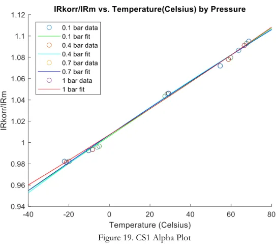
In order to understand the temperature dependence, it was important to find the 𝛼 parameter for each of the three sensors. Several sensor registers were helpful in decoding the temperature dependence and the 𝛼 parameter including the 0x04 𝐼𝑅_𝑘𝑜𝑟𝑟 and 0x0B 𝑀𝑂𝐷_𝑘𝑜𝑟𝑟 registers, where using Table 1, 𝐼𝑅_𝑘𝑜𝑟𝑟 is the 𝐼𝑅_𝑚 signal temperature-corrected at 0°C and 𝑀𝑂𝐷_𝑘𝑜𝑟𝑟 is the MOD (Modulation – non-linearized concentration signal) corrected for temperature at 0°C. 𝐼𝑅_𝑚 gives a relationship between the measurement and reference channels (‰‚•Šƒ‹‚Œ‚•~_{|‚•‚‹‚•Ž‚} ×10,000). In order to obtain the values of this parameter 𝛼, plots of the Jq_•0//_{Jq_s} versus time were first made. The values of Jq_•0//_{Jq_s} at each pressure were averaged after identifying the stable period of reading and reduced into one point. Afterwards, these averaged values of Jq_•0//_{Jq_s} at different pressures were plotted against temperature in degrees Celsius. A linear fit was used to model the data, and the value of 𝛼 used is the coefficient of the 1st_{order parameter in the fitted linear equation.}

Figure 19 is an example of these plots of Jq_•0//_{Jq_s} versus temperature in order to calculate 𝛼 for the CS1 sensor. The fitting equations for the pressures of 0.1, 0.4, 0.7 and 1 bar respectively were calculated as: y0.1 bar = 0.0013x + 1.0060, y0.4 bar = 0.0013x+1.0070, y0.7 bar = 0.0013x+1.0071, and y1 bar = 0.0012x+1.0072. Thus the value of the 𝛼 parameter for CS1 sensor could be used as 𝛼[ = 0.0013.

(42)

Figure 19. CS1 Alpha Plot

Similar process was done for the CS2 and CS3 sensors. However, due to inaccuracies in the readings and experimental errors, the values of the 𝛼 parameter for these two sensors could not be evaluated properly.

After determining the 𝛼 parameter, the previously mentioned b, n and 𝛽7 were calculated. These three parameters were extracted by fitting the KONZ variable to the temperature corrected intensity ratios, I0 and SPAN. Figure 20 shows the fitting plot for each of the CS1 sensors. However, as observed from the plot, due to the large spread in the data, the values of b, n and 𝛽7 could not be properly determined. A similar behavior was observed for the CS2 and CS3 sensors.

(43)

Figure 20. CS1 b, n and 𝛽₇Plot

After the values of SPAN, ZERO, 𝐼7, 𝛼, b, n and 𝛽7 have been calculated, it was important to understand the effect of pressure on the sensor readings. In order to do that, a polynomial of the calculated gas concentration values based on the measured intensities and temperature versus the measured pressure was fit to the data. An n=2, quadratic fit was the simplest function that produced a reasonable fit at low pressure.

Figure 21 and Figure 23 show the KONZ reading for the CS1 and CS3 sensors respectively (multiplied by 0.01). The readings in Figure 21 correspond to a series of 100% CO2 tests where the CO2 pressure was increased from 0.005 bar up to around 1 bar by 0.1 bar increments at a temperature of 20°C. Figure 23 shows a series of 100% CO tests where the COpressure was increased from 0.005 bar up to around 1 bar by 0.1 bar increments at a temperature of 20°C.

In order to understand the pressure dependence of the sensor readings, the start and end points of the stable readings shown in Figure 21 and Figure 23 were identified. Then, the values in each stable period were averaged and reduced into one point each. This allowed us to plot the averaged data points against the known gas pressure in the chamber to quantify the pressure dependence. The pressure fits are shown in Figure 22 and Figure 24 for the CS1 and CS3 sensors respectively. Table 8 is a summary of the pressure parameters for the three sensors.

The same process was done for the CS2 sensor. However, due to inaccuracies in the readings and experimental errors, the pressure dependence for this sensor could not be evaluated properly.

(44)

(45)

(46)

(47)

Figure 24. CS3 Pressure Dependence

Table 8. Pressure parameter A values for CS1 and CS3 (n=2 fit)

Coeff K=0 K=1 K=2

𝐴_[_‘ 25.73 63.53 -2.35

𝐴_’_‘ 72.22 17.16 -0.91

Finally, there was a need to quantify the cross-talk effect happening between the two gases CO₂ and CO. From here, for each of the sensors, a plot of the calculated target gas concentration under the assumption that there is no contaminant versus the known concentration of the contaminant was done, and the fitting equation was used to determine the cross-talk effect. For example, to understand the cross-talk of the carbon monoxide sensor, 0 – 100%, CS3 sensor, a plot of the calculated CO

(48)

values along the x-axis came from prior knowledge of the calibration gas mixture introduced into the chamber according to the values in the previously discussed test plan. Figure 25 and Figure 26 show the scaled CS1 KONZ reading of two different series of experiments, both with an initial CO2 partial pressure of 0.2 bar in the chamber, as CO and N2 are being added every 90 seconds respectively. Then, we plot the averaged data points from the stable period at each pressure increment against total gas pressure in Figure 27 and against the known CO or N2 gas density (in this case the “percent volume”) in Figure 28. A quadratic fit was used to model the data, and the fitting equations are shown in Figure 28. Due to inaccuracies in the experiments, we cannot make conclusive results about the cross-talk parameters—especially for the other two NDIR sensors CS2 and CS3.

(49)

(50)

Figure 28. CS1 CO2 density measured vs. CO or N2 known density

It is important to note here that the SmartGAS sensors are delivered with the values of α and β calibrated at Tcal = 0 °C. Therefore, reading the correct values of concentration from the sensors while on Mars involves three main steps, that are also included in the MOXIE Electrical Interface Control Document Rev G (JPL, 2019):

Step 1: Determine sensor offset and temperature sensitivity

In this step, the effect of the temperature on the value of intensity is calculated. The Mars sensor readings of 𝐼𝑅_𝑚_𝑝𝑟𝑒 and 𝑅𝑒𝑓s are recorded and inserted into Eq. 21 using the previously calculated values of 𝛼 and 𝐼7 for the desired sensor, at the specific measured temperature, 𝑇“.

𝐼 = _q+uJqv”KL

v × JA [1 + 𝛼 𝑇“− 𝑇-E, ]

Eq. 21

𝑆𝑃𝐴𝑁R = 𝑆𝑃𝐴𝑁 + 𝛽7 𝑇“− 𝑇-E, Eq. 22

Step 2: Invert the Modified Beer-Lambert Equation to estimate concentration.

In this step, the previously calculated values of SPAN, b, and n are inserted into an inverted version of the Modified Beer-Lambert Equation to estimate the concentration 𝑥– according to Eq. 23.

(51)

𝑥_– = ln 1 − 1 − 𝐼𝑆𝑃𝐴𝑁R −𝑏

[ —

Eq. 23

Step 3: Implement Temperature, Pressure and Cross-talk Corrections Correction 1: Temperature

In order to correct for the temperature value unit used from degrees Celsius to degrees Kelvin, the previously estimated concentration 𝑥_– is plugged in into Eq. 24 in order to calculate the corrected temperature value of the concentration 𝑋_–.

𝑋_– = R™š(›’.[• R^žŸš(›’.[• 𝑥–

Eq. 24

Correction 2: Pressure

Following the temperature correction, it is important to account for the pressure effect. The sensors’ readings are dependent on the number of molecules in the chamber, which is itself proportional to the partial pressure (CO2Meter, 2015), (Wang, Rödjegård, Oelmann, Martin, & Larsson, 2010), (Gaynullin, Bryzgalov, Hummelgård, & Rödjegard, 2016). As the pressure decreases, the SmartGas KONZ reading of “concentration” would decrease, and thus this effect has to be accounted for. In order to do that, the previously temperature-corrected concentration value 𝑋– is plugged into Eq. 25. Using the previously-calculated 𝐴 –‘ values that range from 𝑘= 0, 1, 2.., 𝑛 where 𝑛 = 2, the new pressure-corrected value of concentration X_– is calculated at the desired pressure P.

X_– = ¢£ W_£‘ F ‘¤A (¥)F\‘ Eq. 25 Correction 3: Cross-talk

Finally, it is important to account for the effect of cross-talk on the sensor readings. In order to do that, the previously calculated value of X– are plugged into Eq. 26 or Eq. 27 below for the desired sensor. 𝑘[ -/0229.E,• and 𝑘( -/0229.E,• are to be derived from the fitting equations of the previously mentioned cross-talk plots.

X_[-0//+-.+¦ = X_[− 𝑘_{[ -/0229.E,•}× X_’ Eq. 26

(52)

under Mars-like conditions, accounting for the temperature, pressure and cross-talk dependence in their readings.

4.1.2 CS4

The CS4 oxygen sensor presents its fundamental raw oxygen measurement data result in the “phase shift” dphi register. It then uses its Settings and Calibration registers to convert the dphi to different oxygen measurement units, including the “mbar” and “% O2” in the mbar and percentO2 registers respectively (PyroScience GmbH).

Based on the theoretical information presented in Chapter 3.2, we plot the Stern–Volmer quenching plots of the JA

J values as a function of partial pressure of O2 in order to quantify the value of 𝐾2o from the slope of the straight-line fit. In order to create these plots, we average the values of J_JA in the stable periods and reduce them into individual points. Afterwards, to satisfy the Stern–Volmer equation, we use linear regression with a forced y-intercept equal to 1. Figure 29 is the Stern–Volmer quenching plots using the series of 100% O2 tests at 70 °C with pressure increments of 0.1,0.4,0.7, and 1 bar. Figure 30 and Figure 31 show the Stern–Volmer quenching plots using the series of 5% CO2 95% O2 tests with pressure increments of 0.1,0.4,0.7, and 1 bar at 45 °C and at 70 °C respectively. Unfortunately, there was a problem in the file where the room temperature experimental data was saved. This missing data is very important for making conclusive analyses about the temperature dependence, thus it creates uncertainty in our analysis of the plots below.

Figure 29. JA

(53)

Figure 30. J_JA vs. Pressure for 5% CO2 95% O2 at 45 °C with pressure increments of 0.1, 0.4, 0.7, and 1 bar