Comparison of three dimensional quasi-linear large swirl theory with measured outflow from a high-work compressor rotor

L. T. Chen and J. E. McCune

by

L. T. Chen and J. E. McCune

GTL Report No. 128 September 1975

This research was carried out in the Gas Turbine Laboratory, M.I.T., supported by the Air Force

Office of Scientific Research (AFSC) under Grant AFOSR-75-2784.

swirling flow in an annulus is applied to predict the outflow from a high-work compressor rotor (1)(2). A comparison of the analytical result with the experimental result is presented. The theory treats inviscid, incompressible flow through a highly loaded blade row in a long annular duct with uniform inlet. Trailing vorticity is shed from each blade

which is represented by a lifting line of bound vorticity. The flow field between successive sheets of voriticity is assumed to be irrotational. The theoretical results are compared to data obtained in the M.I.T. Blowdown Compressor Test Facility (3). The mean circulation distribution is estimated from the mean pitchwise Mach number obtained from the

experiment. The agreement of the predicted mean axial and radial velocity with the experinmental results represents one confirmation of the theory.

The pitchwise-varying velocity are evaluated by the theory at an axial distance of .02 tip radius which corresponds to the probe position if the lifting line is placed slightly ahead, but almost along the trailing edge of the blade. The theory predicts well the pitchwise variation of the velocity due to the effect of shed vorticity which results from the spanwise variation of circulation. The effect is pronounced near the blade tips. Corrections of the theory due to compressibility are omitted here, but will be available shortly.

for the valuable discussions with him during the research period and for his continuous assistance in preparing this report.

The authors are also indebted to Professor W. H. Hawthorne for his

help-ful discussions and the final survey of this report, to

W.

K. Cheng for his enthusiastic assistance, and to

W.

T. Thompkins for his providing the experi-mental data.

I. INTRODUCTION

Due to the three-dimensional nature of the transonic axial compressor, a three dimensional flow theory is required to predict the

pitchwise-varying velocity field. Recently, a newly developed 3-D theory for incom-pressible annular axial flow has become available (2). With several

modifi-cations, this quasilinear theory can be applied to a real compressor design problem with a reasonably large spanwise-averaged loading, and a moderately

large radial variation of loading.

From the Blowdown Compressor Facility developed in the M.I.T. Gas Turbine Lab

C4,

3), a series of experimental results are now available

for comparison with the results predicted by the theory. From the experi-mental results, the distributions of the circulation,

F(r),

and its

derivatives, F'(r), which are related to the mean pitchwise Mach number, can be estimated.

The theory replaces the blade row with a set of lifting lines of bound vorticity and assumes that sheets of vorticity trail downstream of the trailing edge of each blade and are convected away (approximately) by the mean flow. In this way an approximation to the three dimensional flow velocity can be obtained analytically. Correspondinly, the mean

(pitchwise-averaged) flow is treated in the actuator disc approximation. The theory has been separated into two parts: the first is the mean flow theory, which is obtained by taking pitchwise averages, and the

second is the perturbation flow which accounts for the pitchwise variations of the various quantities of interest. The flow pattern is established by considering an inviscid, incompressible flow through the blade row in

an annular duct with uniform and axial-flow inlet conditions. For the mean flow theory, the velocity is described by the stream function, $. It has been shown by several authors that

F

is a function of $ instead of r. The governing equation becomes nonlinear in this case. One way to solve the equation in the case of moderate radial variations of F, is to

approximate

r(p)

by F(r) _{(2). In the present study, however, a more} accurate, iterative process is used to evaluate F($) by successively using the solutions for p obtained in each previous iteration. The consideration of GP(), _{instead of T(r), allows the theory to be applied} for larger radial variations of the blade loading than in Ref. (2).

For the perturbation flow, the discontinuity of the radial velocity across each vortex sheet is prescribed by a sawtooth function (5); other-wise the flow field is assumed to be irrotational between successive vortex sheets.

It should be noted that the present application of the incompressible theory to predict the behavior of the transonic flow is inherently limited. The incoming vorticity, the sonic cylinder effect, and the viscous effect are neglected. The compressible theory which includes the sonic cylinder effect is under study and will be available shortly. The effects due to incoming vorticity can be estimated by additional modifications which will require additional techniques similar to those used in secondary

flow theory. However, the viscous effect is beyond the scope of the present research.

II. FORMULATION OF THE PROBLEM

In the present theory, an inviscid, incompressible flow through a

highly loaded blade row with a finite number of blades in an annular

duct with uniform, axial-flow inlet condition is considered. The blade row is replaced by a row of lifting lines. It is assumed that the

vorticity trailing from the blades is convected by the mean flow. The original structure of the theory was developed by J. E. McCune and

W. R. Hawthorne(l) and by W. K. Cheng (2). However, for the purpose

of predicting the experimental results and taking fairly large radial

variations of circulation into account, F() rather than F(r) is considered.

2.1 Symbols

In this subsection, the symbols used are defined. In order for easy

manipulation, nondimensional symbols are introduced. All the length scales

are divided by the tip radius, rT, the velocity scales are divided by the

far upstream velocity, U_.

For example, the nondimensional radius and axial distance are defined

as

r = (radius)/rT (2.1)

x = (axial distance)/rT (2.2)

The nondimensional absolute and relative velocities are defined,

respectively, as

U = (absolute velocity)/U_ (2.3)

Therefore r = 1 represents the tip radius, =

1

x represents theI far upstream velocity.

The nondimensional circulation is defined as

F = (circulation)/rTU (2.5)

The nondimensional angular velocity of the rotor is defined as

S = (angular velocity) (2.6)

U _Q

2.2 Mean Flow Theory

Belerami flow is applied to the flow field such that (1 , 2)

0 = XV (2.7)

where 0 is the vorticity and can be decomposed as *

Q = 5 + w C2.8)

and V is the relative flow velocity which can be decomposed as IvI

V + v ;- < 1 (2.9)

In the relative frame, the flow is steady and the downstream relative velocity V should be tangent to both the stream surface and the vortex sheet since the vorticity is actually convected by the exact relative velocity V. However, following Ref. 1, we assume the vorticity to be convected approximately by V rather than V and (2.7) becomes 0 XV.

* Bar '-' over any quantity refers to the circumferential average. Small letters represent the circumferential variables.

Also, div V= 0 and therefore

V = V$ x Va (2.101

where $(r,x) is the stream function of the mean flow and

a

is a function defining the vortex sheets*

a = 0 - f(r,x) C2. 11)

The sign of V$ x Va can be determined by considering V while roughly

V$ is pointing in the r^ direction and Va in the

6

direction. Since V-Q = 0, Eq. (2.7) yields

V.Vx = 0 C2.12)

Using Eq. (2.10), Eq. (2.12) holds if and only if

X = X(a,$) C2.13)

Since the flow is assumed to be curl-free everywhere except at the vortex sheets, X can be expressed as the summation of Dirac Delta functions

X = F($) Z 6(a - a) (2.14)

2Tr 4Tr 6T2 where a = 9 BV B..B..., 2

Substitution of Eqs. (2.10) and (2.14) into (2.7) gives

Q = F(i) Z (a - a) V$ x Va (2.15)

Using Eq. (2.15) and taking the circumferential average of Q gives

F=

F(P)

Y

(2.16)

Note the relations (See Eq. (2.6))

=U- S re (2.17)

and

- -= 1 - A 3A D DUr DUx

- = U= -Vx (rU ) x ( rr+ )0 (2.18)

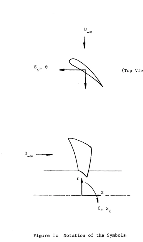
where x^, r, and ^ are the axial, radial, and pitchwise'unit vectors, U

is mean absolute velocity, S is the nondimensional angular velocity,

defined as positive when facing the flow direction and rotating in

clock-wise sense (see Fig.1). U is assumed to be known from experiment; it

is well known that U6 U($) for negligible viscosity.

The circulation distribution 1(r) can be evaluated from

F(r) = r (2.19)

Substituting Eq. (2.19) into Eq. (2.18) and equating the r and x

components of Eqs. (2.16) and (2.18) one obtains

B 1 F B F($) _(2.20)

2Tr r 5r 2T r Dr

B 1 -P B F($) j _(2.21)

2T r x 27r r Dx

Therefore, the function F($) is seen to satisfy

F($) = -- - / rU (2.22)

we ir x

Substituting Eq. (2.22) into the 0 - component of Eq. (2.16) and using Eq. (2.18), one obtains

) + ) = + -1 (2 B.

xr x

or

r r 2TU r r 2rr

v(2.23)

x

This is the governing equation for the downstream mean flow with the boundary condition

A = 0 at r = h, r = 1 (2.24)

where h is the hub to tip radius ratio.

For the upstream flow, the forcing term on the right is zero.

2.3 Solution to the Mean Flow Theory

Eq. (2.23) can be solved analytically if the forcing term is known. In Ref (2) the axial velocity is approximated with the known upstream velocity when evaluating F($) in Eq.(2.2 2).However, this approximation is not entirely adequate for our purposes here. Especially for a tran-sonic compressor, the mean axial velocity varies radially by 30 n 40%. Therefore, an improvement on the approximations in Refs. (1) and (2) is called for.

The solution of Eq. (2.23) is given in Ref. (2) as

2 Xix

r u

+ r A ; x < 0

-X x (2.25)

r+ EA d 1P r z (r) + E B r z (r) ;x > 0

where zlk, are the normalized eigen functions given by a linear combina-tion of the Bessel and Neuman funccombina-tion of the first order:

zp(r) = J CA1 9Xr) + b z Y 1(Atr)/ 1 (2.26)

The eigen value,

A,

and the coefficient b are obtained by satisfying the boundary conditions

z it(1) = z Ch)= 0 (2.27)

and N is given by

N -fr [J Xr)+ b Y (X r) ]2

dr (2.28)

h

The B are coefficients in the Fourier Bessel series which describe the forcing term of Eq. (2.23):

B BF

B _{S, r)(2.29)}B( _TF r) = _F Z Btr z (r)

where

B =r BF() ( S r) z (r)dr (2.30)

it h

Inspecting the above integral equation, one finds in general that B is still unknown since F($) is actually still an unknown function of

4.

However,

by first guessing that U is uniform and equal to unity, (in dimensionless form - see Notation) one can obtain the approximate expres-sion for F($) from Eq. (2.22)

= ($) - (2.31)

r Dr

The coefficients A

u

and A d are related to the known coefficients B , by the upstream-downstream matching condition which requires

Ur

(0 +,r) = U (0,r)

r r

(0+,r) =

:iu

CO ,r)

Applying Eqs. (2.32) and (2.33) to Eq. (2.25) gives B Atu 2 AB d = 9-A 9 C2.32) C2.33) (2.34) C2,35)

Substituting above Eqs. into Eq. (2.25) and taking the derivatives yield the mean axial and radial velocities as follows

B Xx 1+ 2 r r z r) B 1 _{x I} 1+ Z (2 -9 ) r 5 (r _z (r)) rU B X x - E X 9 z (r) 2 =9 - E 9 B z (r) 0

Ue

= r 2 Trr x < 0 (2.36) x >

0

;x < 0 ;X > 0 (2.37) x < 0 (2.38) x >

0

Owing to the approximation given in Eq. (2.31) the results of the first obtained U and U should be corrected by using a more exact

x r

expression for F($). An iterative process is employed by evaluating F('), given by Eq. (2.22), with the above evaluated results of U .

A study of the rate of convergence reveals that three iterations will provide a solution of U _{with maximum relative error smaller than 0.1%}

x

and that a maximum relative error of U larger than 10% will result if no iteration is performed.

2.4 _{Surfaces of the Trailing Vortex Sheets}

The surfaces of the trailing vortex sheets are defined by putting a in Eq. (2.11) equal to a (see Eq. (2.14)). Since the vorticity is assumed to be convected by the relative mean flow velocity, one can locate the surface of the vortex sheet if the mean flow velocity is known. For small x,

r(O _{- a )}

V₆

x (2.39a)

x

where a is the azimuthal position of the blade.

Combining Eq.(2.39a) with Eqs. (2.11), (2.17), and (2.19) gives

BF

f(r,x) (S r - )x/U r) (2.39b)

V 27Tr x

Substituting Eq.(2.39b) into Eq. (2.11) gives

(S BF /r

a ; 6 - (S r - By-) x/(r9 ) (2.40)

V 2Trr x -. 0

2.5 Perturbation Flow Theory

For the perturbation flow, a sawtooth function is used to describe the discontinuity of the radial velocity across each vortex sheet. By taking the curl of the sawtooth function and adding the mean vorticity which drives the mean flow, one will find that the vorticity is zero

everywhere except at the vortex sheet. Therefore a mathematical model of the perturbation flow is fully described.

2.5.1 General Development of Perturbation Equation We start with Eq. (2.15), which can be rewritten as

Q =F(H) (a) V$ x Va

= F($) V$ x VH (2.41)

where H(a) is the repeated step function defined as

H(ca) = 0 -1 -2 0 < < 27r < < 3Tr 3 <r 47r B_ < <~ < (2.42)

Subtracting Eq. (2.16) from Eq. (2.41) gives

V x u F($) [J{ x VH - V$ x Va]

= -

V(H

- a) x

VF

= - VS x VF (2.43)

where Eq. (2.22) has been used and S(a) is called the sawtooth function defined as (Ref . 2) B 1

Sc)

H H(a) - 2'IT a +2 u = V) + A (2.44) C2.45)

Substituting Eq. (2.45) into Eq. (2.43) gives

V x A = - VS x Vr

Let

To satisfy the above equation, one may choose

A = -SS = -S-r (2.47)

The vector A describes the discontinuity phenomenon of the radial velocity across the vortex sheet, appropriate to the inviscid approxi-mation used here.

Applying the continuity equation

V. u = 0 (2.48)

one obtains the governing equation for $

V2 = VSV'r + SV2

C2.49)

with the boundary condition

r 0 at r = h, 1 (2.50)

Consider the order of the first term on the right hand side of Eq. (2.49).

VS.VF _ X -F --f + )r D (2.51)

kt D$ 9x Dx r tr

From Eq. (2.39), the term of 2 is of the order of the axial distance x, which is assumed to be small for present application. The second term on the right hand side of Eq. (2.49) can be approximated as

Using Eqs. (2.51) and (2.52), Eq. (2.49) becomes 3S 9f I

ir

u2p l i'

x r 2 + S ( y +-r ) (2.53)

rU)

x

The forcing term of the above equation can be evaluated when the blade loading and the mean flow velocity are known.

2.5.2 Homogeneous Solution

The homogeneous solution of the Laplace Equation in cylindrical coordinate is given by (2)

ikx.

# = Z Z A A (r) Z np xkinBO (2. 54)

h np np

C.4

p n

where B is the number of blades and

A (r) = 1 {J (A r) + d Y

(\

r)} (2.55)

np

v-

nB np np nB np

np

The eigen values X 's and coefficients d 's are found by

np np

satisfying the boundary condition

A'(h) = A '(l) = 0 (2.56)

np np

The normalization factor Nnp is given by

/1

N

p= jI r {J nBCXn r) + d npY n(X npr)}2dr (2.57) h

2.5.3 Particular Solution

The particular solution of Eq. (2.53) can be found by assuming 0 =inB28

Where the Rn(r) 's are complex and are called the "wake functions", substituting Eq.

C2.58)

_{into Eq. (2.53) and neglecting terms of}

_0(x)

gives 00 { - B (S- BE 2 inB(.9 I 2 + nLL B R I -S n+R

v]}

(2.59) where

In Fourier series, the sawtooth function can be expressed as

S( ) = 1 E sin(nBa) (2.6

Tr n

n

Combining Eq. (2.59) with Eq. (2.53) and using Eq. (2.60) gives

2Rn 1 DRn 2 2 BF -2 1 Dr"+r r nB [(S- 2 -r +-2] = Gn (2.6 B B( r a U +r 1 2Dr ( 2 .6 G (-)+

i

( - + - r)

(2.6:

GnT) -r Dx (rU )2 nTT r x n = 1,2, 3,... 0 0) 1) 2)

In Ref. (2), the radial velocity is assumed to be small and the first term on the right of Eq. (2.62) is dropped. However, for a large number of blades, this term becomes significant and should be kept.

2.5.4 _{Homogeneous Solution of the Wake Function} Upon the transformation

Rn(r) =

Equation (2.61) with Gn(r) = 0 becomes

$n (r) - n2B2P 2(r)$ n = 0

(2.63)

where

P(r) r C2.65Y

and w(r) represent the local tangent of the outlet flow angle or,

w(r) = S r - BF (2.661

V

27r

The asympototic solution of Eq. (2.64) is given by 1 nBfrp(r)dr

n(r) = - 0 _{C2. 67)}

nBP(r)

For typical compressors, the number of blades, B, is large, therefore, the error of the asympotic solution is small.

2.5.5 Complete solution of the wake function

Two homogeneous solutions of Rn(l) are given by Eq. (2.67) as

Rn1(r) = 1 nB rp(r)dr (2.68) 1 (r= nBrP (r) and r Rn (r)= 1 -nB p(r)dr (2.69) 2 nBrP(r)

One

can obtain the complete solution of Rn(r) in terms of two independent homogeneous solutions as follows

R i(Q) G (O) Rn(r) = CnRnl (r)+ D R 2(r)+ R 2(r)

$

nl( d

n _{R (C) G (2)}

+ Rni(r) f n2 WnOn dC (2.70)

The wronskian Wn(r) is found to be

W (r) = W (l)/r (2.71)

n n

or Wn(r) = R (r) R (r) - R 2 (r) Rn (r) (2.72)

By numerical integration, two integrals in Eq. (2.70) can be evaluated. The coefficients C and D are obtained by satisfying the boundary conditions which read

Rn'(1) = Rn'(h) = 0 (2.73)

2.5.6 _{Perturbation Velocity Component}

By combining Eq. (2.54) with Eq. (2.58), the velocity potential

p

is given as X x. E Z A u A (r) k np x inB , x < 0 n p np np $n p (2.74)

~

u Ap (r L nBOen~ Z E A np A () np nB1 + Z Rn(r)Q ' x > 0 np np n p n Xx To satisfy the far upstream and the far downstream condition, k np -X x

and Znp terms are chosen respectively for the upstream and the down-stream solutions.

Substituting Eq. (2.47) and Eq. (2.74) into Eq. (2.45) gives

E E A u X A (r) k np inB ; x < 0 In pnp np np u = _(2.75) -A x iB nc E E -A d A A (r)kL np x B, + E(inB)R (r)

ZinB

;

x > 0 np np np np n Dx

A .

A 'A , Cr)' A n 1B x < 0

np np

U = (2. 76)

U rA d ,(r)X npx iBO inBa Dr Sin(nBa()) x .>0

n. np np r nTr

E E A U(inB)A (r) np inB 0

n p

U= (2.77)

SZ A d (inB)A (r) X np xkinB + E(inB) Rn(r)R ;inBo x > 0

n p np np

In deriving Eq. (2.75), terms of 0(x) are neglected. As we did for

u d

the mean flow velocity

he

coefficients A u and A d have to be determined

np np

to satisfy the upstream and downstream matching condition which requires

u (x = 0+) = u (x = 0-) (2.78)

x x

ur (x = 0+) = ur (x = 0-) (2.79)

In order to match the upstream and downstream condition, terms of nBRn(r) in Eq. (2.75) and terms of Rn(r) + '(r) i in Eq. (2.76)

should be expanded in terms of Fourier-Bessel series as

i n B Rn (-) = 2 a A (r) (2.80) x pnp np p Rn(r) + F(r) i= b A (r) (2.81) nTr np np p where I 1 a = inB Rn(r) -) r A (r) dr (2.82) np x np

b =fIRnr) + ii r A Cr) dr (2.83)

np nT np

By substituting Eqs. (2.80) and (2.81) into Eqs. (2.75) and (2.76) respectively and applying the matching condition given in Eqs. (2.78)

and (2.79), the coefficients A u and A d can be calculated as follows.

np np A u ( + b ) (2.84) np 2 X np np A d ( - b ) (2.85) np 2 A np np

Further details of this development are available in Ref. (2). In Ref. (2), the first term in Eq. (2.62) is omitted for the case of negligible radial velocity, therefore, Rn(r)'s are pure imaginary, bnp's are pure imaginary and anp's are real.

III. CORRELATION WITH THE EXPERIMENTAL RESULTS

The formulations given in the previous Sections are intended to

predict the velocity field very near the blade row with heavy loading,

provided that the distribution of the loading on the blade can be calculated. It is the purpose of this report to investigate the three dimensional structure of the flow field behind the 23-blade rotor of

the Blowdown Compressor facility, developed in the M.I.T. Gass Turbine Lab, and to present a comparison of the analytical results with the

experimental results. The loading distribution is obtained by taking

the pitchwise average of the measured pitchwise Mach number, in accor-dance with Eq. (2.19).

3.1 Blowdown Compressor Facility

The blowdown compressor facility consists of a supply tank, initally

separated from the compressor by a diaphragm, the compressor test station and a dump tank into which the compressor exhausts. When the diaphragm

ruptures, the gas expands from the supply tank, which essentially behaves as a stagnation plenum. This requires that the test time be large compared to the acoustic period of the supply tank. As the supply gas expands, its pressure and temperature decrease and by proper control of the system,

the rotor tangential Mach number can be made nearly constant throughout the test time. If the compressor discharge orifice remains choked, this

in turn implies that the axial Mach number is constant (4).

An overhung rotor without inlet guide vanes, with an inlet hub-tip radius ratio of 0.5 and outlet hub-tip radius ratio of .64 Csee Fig. 2),

a tip tangential Mach number of 1.2, design pressure ratio 1.6 and radially constant stagnation temperature rise were selected.

During the experiment, the 23-blade rotor with diameter of 2 ft. is turning at 166 rps (4).

3.2 Experimental Results

A specially developed, fast response four diaphragm probe was used for the survey of the downstream flow field. All the experimental data presented here are extracted from Ref. (3) and were obtained by

W. T. Thompkins and Prof. J. L. Kerrebrock. By traversing the probe through a small free jet and monitoring the response of four diaphragms, the three components of the flow velocity at several axial stations can be described. Meanwhile, the mean flow velocities are obtained by taking

the time average of the probe response (Ref. (3)).

3.3 Circulation Distribution and the Shed Vorticities

The azimuthal variation of the velocity components, in our theory, is due to the shed vorticity which, in turn, is due to the radial non-uniformity of the blade loading. Therefore, the first step in application of the theory is to determine the circulation distribution.

From the definition of the nondimensional circulation, one obtains (see Eq. (2.5))

F(r) = 27rU 2Trr. (3.1)

B _{B 1}

x

where the mean pitchwise Mach number, Me, is acquired from the experiment and the axial Mach number at far upstream R4 is assumed to be uniform

and has value of 0.5.

After obtaining the circulation distribution, V(r), the first and the second derivatives of the circulation, F'(r) and P"Cr), can be

evaluated by the finite difference method. The value of I'(r) is assumed to be the strength of the shed vorticity. Fig. 3 presents a curve of mean pitchwise Mach number which was chosen as the basis of evaluating F(r) and compared with the experiment results which are obtained at port

*

5 (Ref. (3)). Fig. 4 presents the distribution of T(r) evaluated by Eq. (3.1) and the distributions of F'(r) and F"(r).

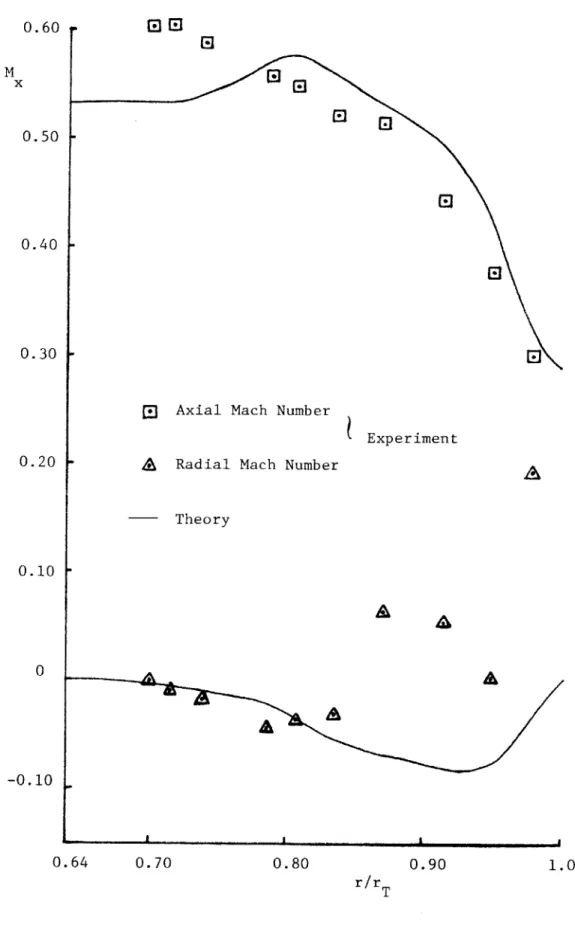
3.4 Mean Flow Velocity

The mean flow is the superposition of the unperturbed uniform inlet flow and the mean flow which is induced by the mean trailing vorticity with strength of P'(r).

Since values of

T'(r)

are given in the above section, the mean axial and radial velocities can be evaluated by using Eqs. (2.36) and (2.37). As mentioned in Subsection 2.2, an interative process was adopted to

improve the results beyond those obtained from a linearized forcing term. Four iterations are performed. The final relative differences between successive iterations are smaller than 0.1%. With mean pitchwise Mach number, obtained from experiments, as an input, the analytical

results of mean axial and radial Mach number are calculated as an output and compared with the experiment results. The comparisons are presented in Fig. 5. The agreement between the analytical prediction and the

*

experiment results is good for the mean axial Mach number, but not for the mean radial

Mach

number for r> -8r which is near the sonic radius. For

T

the mean axial Mach number, the agreement is fairly good in the range from .75r to rT and shows the correct trend. The larger deviation between the two results near the hub may be due to a separation near the hub

and the non-uniformity of the inlet velocity. For the mean radial Mach number, the deviation between the two results near the tip is large (in

relative terms). This is evidence of strong viscous effects not included in the theory; indeed these viscous effects may be accentuated outside

the sonic radius of the experiment because of shock-boundary layer inter-action.

3.5 Perturbation Flow Velocity

The downstream perturbation flow is assumed to be the superposition of the potential flow and the solenoidal flow. The former is evaluated from the velocity potential given by Eq. (2.74) while the latter, which in our approximation has only an r component, is described by the saw-tooth function given by Eq. (2.47). The total axial, radial and pitch-wise velocity are obtained by adding Eqs. (2.75), (2.76), and (2.77) to

Eqs. (2.36), (2.37), and (2.38) respectively.

Although the solution of the perturbation flow theory is compli-cated, a simple picture of the flow pattern can be obtained by considering a large number of blades. In Eq. (2.61), the first and the second derivative terms can be neglected for large B, and the solution of Rn(r) is then

1 DF Dr

proportional to - (r-). Compared with the term of S-, the Rn(r)

T~-r:

~r

term is negligibly small except very near the tip where the theory can not be applied properly. Therefore Rn terms in Eqs. (2.74) to (2.77) can

be neglected for large B, and the coefficients of the duct modes comes merely from the effect of S-. This can be observed from the Figs. 7a to 10c explained in the following section.

3.6 The Axial Distance

Given in Eq. (2.74), the velocity potential, , can be separated into the decayed part, which includes the exponential decayed term,

-X x

k np , and the undecayed part, RnCr) terms, which remains undecayed along the axial direction. The former dominates the solution for flow field near the blade row, while the latter represents the far downstream

*

solution.

A study of the velocity at several axial distances, x/rT = .02,.05,

.10 and

o,

is presented in Figs. 7a to 10c for four radial stations, r/rT = .785, .805, .845, and .95 with pitchwise stations going from

the pressure side to the suction side. From the figures, it is shown that the pitchwise variation of the downstream velocity are decreased by a factor two to twenty for x varying from .02rT to .lrT. For axial and

pitchwise Mach numbers, the contribution of Rn(r) terms cause the pitch-wise variation far downstream or x/rT =

x.

For the radial Mach number,

the contribution of the Rn(r) terms represents the deviation from the sawtooth function at X/rT = o. As we expect, in the figures the Rn(r)

contributions are quite small. Since the pitchwise variation of the down-stream velocity decayed from infinity to almost zero for x within the range from 0 to .lrT, it is important to choose a reasonable value of x

*

The theory given in this paper is valid only for small x. The words, 'far downstream', are merely chosen to represent the undecayed part of the solution.

which- corresponds to the physical probe position where the experimental results are obtained. By careful comparison between the pitchwise

variations of the experimental results and the analytical results at

several axial distances, the value of x is chosen as .02rT which roughly corresponds to 0.12 axial chord length downstream of the rotor. The

experimental data were obtained at 0.10 axial chord downstream of the rotor; therefore, the corresponding location of the lifting line would be slightly ahead of, but very near, the trailing edge of the rotor blade.

3.7 Rate of Convergence of the Series Solution at Different Axial Distances It has been mentioned previously that the present theory is valid

for small axial distance from the acuator disk position. However, the value of x can not be chosen as small as we like because if the value of x approaches zero, the series solutions given in Eqs. (2.74) to (2.77) become divergent. It is the purpose of this section to choose a reasonable number of terms of the series solution which converges with small relative error for the desired value of x.

First, the convergence problem for small x is considered. To simplify the problem, consider the case for large B as in the discussion given

in the subsection 3.5. Compared with term of

S

, one may assume

Rn(r) << S-- (3.2)

Tr

Therefore, comparing Eq. (2.80) with Eq. (2.81) gives

and

bnp - 1 rA (r) dr Snff _np

From Eqs. (2.82), (2.84), and (2.85), one obtains

_u,d + bnp

n P - 2

In the approximation yielding (3.4) we have simply b

bnp n

In order for the series solution of u , given in Eq. (2.75) to converge for p = 1, the necessary condition is

Xnp Z,

-kx

np _{< n (3.7)}

lp

Consider the first eigen value which is approximately

(3.8) Xnl 4 n B -Ax np K (x) = K(n,x) = np n n

-p

x i p (3.9)

the axial velocity can Lhen be rewritten in terms of Kn(x) as

(3.10)

oo b _{-Xy x N}

iB

U =E - - lpx {f K (x) A (r) ZinB}

x p2

lp

n np

where terms with n larger than N are dropped. Substituting Eq. (3.8) into Eq. (3.9) for p = 1 gives

(3.4)

(3.5)

(3.6)

Kn(x) = Bx (3.11) nBx

It is obvious that in order for the series

u

to be convergent Kn(x) should always be less than unity, or

K(n,x) < 1 (3.12)

The above condition is satisfied for any value of x except x = 0. Furthermore, from Eq. (3.11), it is noted that the smaller the value of x is, the slower the convergence goes. Therefore, a proper value of x

should be chosen to give the required convergence with a reasonable range of n.

In Fig. 6, the curves of function K(n,x) for p = 1 versus n at several different axial distances x are plotted. From the figure, one may conclude that to obtain almost zero relative error for x = 0.05,

N = 6 should be chosen; for x = .03, N = 9 should be chosen; and for

x = .02, N = 13 should be chosen. However, it should be noted that if

Ba

the number of n increases, the errors induced in expressing nB Rn(g-), Pr'

or Rn +

-i--,

in terms of Fourier-Bessel series are also increased, and meanwhile the computing time for large n increases sharply. Therefore,

for the present purposes, x = 0.02 and N = 6 are chosen for calculation. The relative error caused by dropping terms with n larger than N can be estimated by the area under the curve. The relative error is equal to the area under the curve from n = N to n =

o

divided by the area under the curve from n = 1 to n =

o.

For the present choice of n and x, the maximum relative error is about 10% for p = 1.

1 * For fixed n, the magnitude of b decreases at a rate of (-v)

np p

Therefore the magnitude of Kin,x) as well as the error induced by dropping terms larger than N also decreases at a rate of (-2). Summation of the

p

errors for different p gives approximately 15.5% as the total maximum relative error for the present choice of N and x.

It is also important to note that the above criterion is obtained based on the assumption that Rn is of order c. However if Rn becomes significantly large (for example, near the tip), the above criterion is

1

still valid, because Rn converges at a rate of (-s) which is much faster n

than (1), the convergence rate of the coefficients bnp.

3.8 Complete Velocity of the Flow

In Figs. 11-19, the mean flow combined with the pitchwise variation of the radial, axial and pitchwise Mach numbers, evaluated at x = .02 rT' for radial stations r/rT = .700, .715, .738, .785, .805, .845, .870, .915, and .95 are presented and compared with the experimental values. The

blade passing period goes from the suction side to the pressure side. The distance of unity along the blade passing period represents one blade spacing.

The pitchwise variation of the flow velocity near the hub, for

instance r/rT = .700 and .715, is much smaller for the analytical results than for the experimental ones. This may be due to the strong inlet

vorticity which was not taken into account in the theory. However, for the more outboard radial stations, the agreement between the analytical

This is the conclusion obtained directly from the calculated results of the coefficients, bnp in Eq. (3.4). No attempt has been made to prove it mathematically.

and the experimental results is satisfactory, if we can interpret the upward jump of the axial Mach number and the downward jump of the tangential Mach number as the effect of the viscous wake of the blades. The achievement attained here is that one may identify the effect due to the trailing vorticity by comparing the pitchwise variation of the analytical and the experimental results. This seems to represent a step forward in the state of the art, since, so far as the authors know, the pitchwise variation of the velocity for an actual high work axial compressor blade row has not been predicted previously with this relative degree of success, other than by strictly numerical procedures. Even so, it is clear that the theory still requires considerable improvement to allow for effects so far omitted.

IV. DISCUSSION AND CONCLUSION

The three dimensional theory for incompressible, inviscid flow through an annular duct is applied to predict the velocity behind a transonic compressor blade row.

The radial loading distribution of the blade is estimated from the mean pitchwise Mach number, and the correctness of the estimation is relatively well confirmed by the comparison of the predicted mean axial velocity with the experimental one. The prediction of the mean radial velocity is comparatively poor for the flow region near the tip. Aside

from the viscous effects previously mentioned this may be due to the tip effect which causes outward radial flow, or due to secondary flow, or possibly compressibility effects yet to be included in the theory.

The pitchwise variations of the axial, radial and pitchwise

Mach

numbers are presented and compared with the experimental ones. For the radial stations away from the neighbors of the hub and tip, the analy-tical results seem to be able to predict relatively well the effects due to the vortex sheets. However, the effects due to the separation of the boundary layer, which are not considered in the theory, are seen to

be as important as the effects due to the vortex sheets. The unexpectedly large jumps of experimental data in Figs. 9b, 10b, llb, and 12b are

believed to be the result of the viscous wakes of the blades.

For flow near the hub, the inlet vorticity is intensified because the hub radius varies from zero to .64rT within an axial distance of .6

rT' The vorticity caused by the large hub-radius variation is significant

and probably dominates the flow field near the hub where the shed vorticity due to the nonuniformity of the loading is quite small. This may help explain why the variation of the analytically predicted results given in Figs. lla % 13b is much smaller than the experimental result.

APPENDIX

COMPUTATION AND COMPUTER PROGRAM A.1 Bessel and Neumann functions of large order

The cylinder functions, A (r)'s, are a linear combination of Bessel np

and Neumann functions. Their properties are fully described in Ref.(6). In seeking formulas for the Bessel and the Neumann functions of large

*

order

and their derivatives, the following asymptotic

expansions

are used 1 J

(nz)

=

(

4

/3

n =lz 4/3 n 1 Y '(nz) =

₍

_{) 4 14/3} n 1 J '(nz)=(A.₂

)1

1 Y '(nz) =-(4 z 4 1 n 4/3 n {Ai(n 2/30 + 'Ai' (n 2/3 h /3 {Bi~n/35)+ Bi(N ) /3 n

{Bi(n2/3) + Bil(N 2/3 ) bo0

{Ai(n 2/3 g/3b n 2/ 2/o {Bi(n /3 2/3 n + Ai'(n2/3 + Bi'(n 2/3)

Ai, Ai', Bi, and Bi' are Airy functions

can be obtained from available tables.

= f( n V+/-z2 2 _/3 _;

_Izl<

3 z cos-11 2/3

2 z

and their derivatives

0.999

;zf> 1.001

*

See "Handbook of Mathematical Functions with Formula, Graphs and

Mathe-matical Tables", p. 368.

In order to obtain the required accuracy for 1.001 < z < 1.01, following formula is used -1 3 3 32 52 +.... co~(-) - a + -+ a. 32 7 +... COS z 6 5! 7! where a z- /Z where which

and

B = IK-1/2 {0.125 1z2 l -1/ 2 + 0.208333 Iz2K-3/2} -0.104167 12

C₀ = -/2 {0.375 z2 -1/2 + 0.291607 1z_ -3/2} + 0.145833

For .999 < z < 1.001, Jn, Yn, Jn' and Yn' are approximated as functions of n only. Details of the approximations are given in the Handbook of Mathematical Functions.

A.2 Numerical Integration Involving Exponent of Larger Argument

In evaluating the integrals in Eq. (2.70) numerically, the exponent of large argument is involved. In order to avoid an overflow of the computer, all the exponential terms with positive arguments are divided by exp (7.0*N) while the exponential terms with negative arguments are multiplied by exp (7.0*N). The division and the multiplication factors

are cancelled with each other at the end of the calculation.

The numerical results of the integrals are obtained by separating the integration interval into two equal intervals. For each interval, 25 Lobatto points are used.

A.3 Introduction of the Computer Program

The computer program is divided into three parts which are described subsequently.

The first part of the program generates the eigen values and the normalized cylinder functions which are written on a tape and, later, are

read in from the tape in the second part of the program. The subroutines used include

BLOCK DATA INPRE KE2GEN ROOTS FUNCTY BESSF BESSD AI AIP BI BIP LOBATO BESJ BESY

The last two suhroutines BESJ and BESY are in the IBM SSP package. In the second part of the program, the eigen values and the normalized cylinder functions are read in from the tape and the velocity potential, the wake function, and, finally, the total velocity are evaluated. The velocity distributions are written on a tape for plotting purposes in the third part of the program. The subroutines used include.

MAIN BLOCK DATA INMAIN GAMAIN MNFLOW PTFLOW INTEXP OUTPUT LOBATO MISC PHIS DEBUG

The third part of the program is a plotting program which involves a Calcomp offline pen plotting system. The plotting system consists of a Calcomp model 563 Incremental Digital plotter and a Calcomp model 905 controller which are manufactured by California Computer Products. This package, available at the MIT Computer Center, is used for plotting the Mach number distribution along the azimuthal stations. The subroutines used include

MAIN INPOST DEBUG BLOCK DATA PLOTS PLOT PICTURE SYMBOL NUMBER ENDPLT

The last six subroutines are Calcomp plotting subroutines.

A.4 Input Data to the Program

In the first part of the program, the input data are read in by a namelist statement, 'INP'. The following input data are included:

IOD Reference number of the Data file to be read from. The default is 5.

IOW _{Reference number of the Data file to be written on. The} default is 60. The write statement is skipped if

IOW

= 0. IOP _{Reference number of the print file. The default is 6.} NBLADE Number of the blades.

H Rub to tip radius ratio.

IGENN _{Number of the cylinder functions with order other than unity.} The maximum number is 6.

IGENP Number of the eigen values for each cylinder function with order other than unity. The maximum number is 15.

IGENMN _{Number of the eigen values for cylinder function with order} of unity. The default is 6.

ACCUR Required accuracy of eigen values.

In the second part of the program, there are two read statements which read namelists 'INM', and 'PIN'. In the namelist 'INM', the

IODR Reference number of the data file where the eigen values and cylinder functions are stored. The default is 60.

IOW Reference number of the data file to be written on. The default is 61. The write statement is skipped if IOW - 0. IOP Reference number of the print file. The default is 6. SNU The nondimensional angular velocity, defined in Eq. (2.6). XDATA Axial distances to be used in computation. The default is

.02,0,0,0,0,0,0,0,030.

NXSTEP Number of axial distances, the default is 1.

KODING Series expansion, instead of exact sawtooth function is used if KODING smaller than 10; Rn(r) is ignored if KODING greater than 5 and smaller than 15. The default is 20.

NTHETA Number _{of azimuthal stations. The default is 26. The maximum} is 26.

IGENN Number of orders of cylinder function except order of unity, the default is 6.

IGENP Number of eigen values, the default is 15.

INDEX Define the seventeen radial stations used for velocity compu-tation from 49 Lobatto points. The default is 1, 8, 14, 18, 21, 23, 24, 25, 26, 28, 30, 32, 34, 36, 39, 42, 49.

RWITE Define the radial stations for velocity print out. The default is zero.

In the namelist 'PIN', the following information are read in.

RGAMA Define seventeen nondimensional radii where the circulation is evaluated.

GAMA Define the nondimensional circulation, in Eq. (3.1) at each radius defined in RGAMA.

CGAMA Define the mean value of GAMA.

For the third part of the program, input data are read in by a namelist, 'int', which include the following input data:

IOR Reference number of the data file to be read from, the default is 61.

IOP Reference number of the print file, the default is 6.

IXPLOT Index for plot at each axial distance, the default is 0, no plot for the referred axial distance.

RPLOT Radius where the desired results are plotted. When the default is 0, one obtains no plot for the corresponding radius.

UMACUZ Mach number at far upstream. IDUMI, IDUMNZ, IPTF

Calcomp index, the defaults are 30, 30, 9.

It should be mentioned here that some of the subroutines used here are the results of the cooperation with W. K. Cheng (2) and some of them resulted from the modification of his own subroutines.

REFERENCES

1. McCune, J. E., and Hawthorne, W. R., "The Effects of Trailing Vorticity On The Flow Through Highly-loaded Cascades," paper accepted for publica-tion in J. Fluid Mechanics.

2. Cheng, W. K., "A Three Dimensional Theory For the Velocity Induced by A Heavily Loaded Annular Cascade of Blade," S.M. Thesis, MIT, June 1975. 3. Thompkins, W. T. Jr., and Kerrebrock, J. L., "Exit Flow from a Transonic

Compressor Rotor," Proc. AGARD Propulsion & Energetics Panel 46th Meeting, Monterey, 22 -26 Sept. 1975, Paper No. 6; also MIT Gas Turbine Lab. Report No. 123, Sept 1975.

4. Kerrebrock, J. K., et al., "The M.I.T. Blowdown Compressor Facility," ASME Paper No. 74-GT-47.

5. Reissner, H., "On The Vortex Theory Of The Screw Propeller", J. Aeronauti-cal Sci., 5, 1, Nov. 1937.

6. McCune, J. E., "A Three-Dimensional Theory of Axial Compressor Blade Rows -Application in Subsonic and Supersonic Flows," J. Aero/Space Sci., 25, 9, 1958.

U S v, 0 (Top View) U r

8,S

U0.

0.5 r T 0. 64 r T

-_

_ Lr

Actuator Disk (mean flow)

Lifting Line (perturbation flow)

M_0=0. 5 r T r _{0.64 r T} r x - -x

E Experiment Assumed Curve

(input to the theory) 0.50 M 0.45 0.40 0.35 0.30 0.64 0.70 0.80 0.90 r/ _rT

Mean Pitchwise Mach Number

Ea

ID

/ I

8

El

1.00 i A Figure 3:

1.4 F (r) 1.3 1.2 1.1. 1.0 0.9 0.8 0.64 0.70 0.80 r/rT 0.90 1.0 F(r) distribution Figure 4:

Mx

0.50

0.40

0.30

0

Axial Mach Number

SExperiment

0.20 Radial Mach Number

Theory 0.10 0 -0.10 0.64 0.70 0.80 0.90 1.0 r/rT

0.80

0.60

0.4(

0.2(

5

Figure 6: Function KIn,x)

-\+

+

+

'

'

RT R/RT=0.785

a

X/RT=0.020

n

X/RT=0.050

X/RT=0. 100

+

X/RT=CO

(D'

CO

CO LO Ir -co Ln C7 Lo CO CJO 1 6 11 16 21 26

PITCHWISE

STRTIONS

Figure 7a

*

X/RT=O.020

*

X/RT=4.050

&

X/RT=O.

100

+

X/RT=CO

Cs co

co

cJ.

zLCD

CECH

S

ST.I0N

C\J LrD CD

61

16

21

26

PITCHWIBE BTPTIONB

Figure 7b

HT R/RT=0.785

+ Lfl

X/RT

X/RT

X/RT

X/RT

=0.

=0.

=0.

=co

020

050

100

11

PT

TCHWJSE

16 21

STRTIONS

Figure 7c

r

ULJ

cm

(-r) m Co) CD) m~

l1

₆

₂₆

zc ISr", !Sr- 01111, -4 i i

n

X/RT=0.020

r

X/RT=0.050

X/RT=-0.100

+ X/RT=CD

co Lfl ~+ + co cc) co CNd Ccc

CE

LU CD uX ~D L

-

1

6

11

16

21

26

PITCHWISE STRTIONS

Figure 8a

RT R/RT=0.805

a

X/RT=0. 020

o

X/RT=0. 050

&

X/RT=0. 100

+ X/RT=QJ

c

r -LLJ

~Zr

-E

16

11

16

21

26

PITCHWISE

5TFRTIONS

Figure 8b

X/RT=0.020

o

X/RT=O.050

X/RT=O. 100

+

X/RT=CD

Lfl m rr) LIi CC)2 LLJ co Lii

n

C\J CDJ r\J

611

16

21

26

PITCHWISE

STRTIONS

Figure 8c

RT

9/RT=0.845

,

X/RT=O.020

o

X/RT=O.050

a

X/RT=D. 100

+

X/RT=CD

+ + 1 1 i C) U-) LLJ LO Cc

~Z

C= Ln-~IU Cr) Lfn

1

6

11

16

21

26

PITCHWISE STRTIONS

Figure 9a

a

X/RT=O.020

e

X/RT=O.050

X/RT=G.

100

+

X/RT=CD

uO

U-C CELJ CCLo U-) L)

6

116

21

26

PITCHWISE STRTIONS

Figure 9b

PT

R/RT=0.845

m

X/RT=O.020

e

X/RT=O.050

SX/RT=O. 100

+

X/RT=C

CD -) Z

cr

Li U5-'j rr-cnCD rr) Cr)

6

11

16

21

26

PITCHWISE STRTIONS

Figure 9c

o

X/RT=O.020

o

X/RT=0.050

a

X/RT=O.

100

+

X/RT=CO

CD U-) m Lo cc U-) K-) CD L) COj m crn

6

11

16

21

26

PITCHWISE

STRTIONS

Figure 10a

RT

B/RT=0.950

m

X/RT=0. 020

o

X/RT=0.050

&

X/RT=0. 100

+

X/RT=CD

cm r\j LJ

ci:

cn (\j

1

16

21

26

PITCHWISE

STRTIONS

Figure 10b

+ LO)

x

x

x

x

/RT=0.

/RT=0.

/RT=0.

/R T=CCD

020

050

100

11

P1 TCHWJSE

16

STPTIONS

Figure lc LUJ Z LJ

cn

C. U-)

,-1

6

21

26

I - I .-- --4. .4 - -.4 4-... jjjj'

DOWNSTRERM

X( EXPERIMENT THEORY I"

x

x x

x

x

_{x v}

x

x x xx x x

0. 60

B

L

A D E

p

20

Pq5

1. 30

2.40

SING PERIODS

0 U-,

1

U)

xX

x

x

w

z

U cc 0 M ri'

0 .

.CI0

3.00

3. >00

t4.

30

AL EXPERIMENT THEORY 0 r-%. 0 C IL~ + _r.r + + r4 4-' 7 7-I +4?-1 + r. r 4 ₄.JY4_.r- f 4 -r -I- .4. cm 0 Ln) "Al e~.1~ 4 ei .j *.

~ ~

Mo Ca.1 .1 I,, 1^ i.e ,4;A

1

20

LPCE PRSSIN

X: LU ILL W, U 0-.4 _+I Ul .4. (n LUJ z U cc

Th. oo

B

A ~4I~ ~4~

I

G

(90

P ER

2.

j 40

1005

3.-00

3.3()

4.

20

~.

CHORDS DOWNSTRERM

OF ROTOR

X

EXPERIMENT THEORY I' x x x x x x x x xx

xx

x

x x x* x Sx x

0.60

1.

20

BLADE

PRS

1.

SING

30

PE

2. 40

IODS

0 0 K.

x

x x

x x

L&j U -j 0n 0 0 0\

0. (.

0

3.00

3.60

14.20

4. (f3

THEORY -rr !4- +~t-t,. 4. 31~~~~ .3. ,J. 3 .113 -J I I I 0.5 0 1 120

BLPOE PPSSIN

I

(0 2.40

G

PERBIODS

LU cr LU a_ 0 0 + 0 co

5 7

0n c0 U-1 LUJ z U cr 33 3.3 ;U4,1*3

T'.

00 3. 00 3.650 q,1 20 L I

0

d.

r'j I ...

₀

x

EXPERIMENT THEORY I C-) x_{x x x} x x x x x x

x

x x x

0.

00

0.70

1.4q

2.10

2.0

BLAIDE PFV33ING PERIODS

3.U)

4.20

L'3(

I . L U) LUJ cr -cr

+ , A EXPERIMENT -... THEORY C z CU CL. LUJ z U Li -J: t~f) iC-e - . -I H 21 C)2 Lq BCD F '5I G)R D

OROS

OF

ROTOR

)( EXPERIMENT .. THEORY I'3 C) xx x xx

x

x

x

No

x

x

x

No

x

>;x

X

xx x x x

&

5 x l

Cxx

*<

x

xW x xt 0.

70

1.4c

-BLROE

PRSS

2.

I

NG

I

C)

PEPI 0

x r , CD c 2 cc LU cz cc b-4 D

0.00

_{2. ~30}

05

3. 50

L.

90

.

(5(

I

+ A EXPERIMENT THEEORY C, 41 z ₊₄ -4-I -+ _+.:+

_g

+ -r L)J

.r~7

0- ' UjIrk,

0.M4

3%I1905f,

DOWNSTRERM

OF ROTOR

X EXPERIMENT - . THEORY on x xx x x Vx

0. 70

1 q 0

BLPDE PRS

SING PERIODS

2. 10

2.80

Lo M -LJ X: (xiI 0

.00

3, 50

4 .

20

4 90

5. 5U

I

+,AEXPERIMENT

~THEORY

7I-f+ 4-+-+ *1*4~ '~;- 4 .4 + 4 + +

~1~-r

_*1*

~

r#.~I~i-+A _{T f+} 4- 4r A ly a64-Ago) 6. le?. 7A :.~ ;~&I a 'a

I0.70

.BLFAOF

1.14

p

R5

2.1

I

NG PEBJ1O

.4. -r 4 + LJn C C (D Lo 0 4+ cc L&U L) U -0.. U z U cr + ~rt -r Ul C4

00

o

_{2.F J0}

_{I3. SO}

os,

4.20

14

90

5 .

60

C

I

M

0

ry,

0. 1

RXIRL

CHORDS

DOWNSTRERM

OF ROTOR

X EXPERIMENT - THEORY x xx

x

X-.- X x

vqmx

< x X, x x X X _{x Xo} x x

1

.

40

ROE PRSS

2. 10

ING

PE

RIODS

4

. 90

C71 cc U, a: cr a:

0. 00

0. 70 .

BL

3.

j0

4.

20

5. 60

____THEORY 0 ,. -r U + - + 44. r4 *f LU .1~- .

~

7 r~4r r 4r- fT. rr +~ U .0 C1"C .1 70 1 l 2 j 1 c)2 903 5 0q 9