HAL Id: hal-02270001
https://hal.archives-ouvertes.fr/hal-02270001
Submitted on 23 Aug 2019
HAL is a multi-disciplinary open access
archive for the deposit and dissemination of
sci-entific research documents, whether they are
pub-lished or not. The documents may come from
teaching and research institutions in France or
abroad, or from public or private research centers.
L’archive ouverte pluridisciplinaire HAL, est
destinée au dépôt et à la diffusion de documents
scientifiques de niveau recherche, publiés ou non,
émanant des établissements d’enseignement et de
recherche français ou étrangers, des laboratoires
publics ou privés.
Atlas-Based Automatic Generation of Subject-Specific
Finite Element Tongue Meshes
Ahmad Bijar, Pierre-Yves Rohan, Pascal Perrier, Yohan Payan
To cite this version:
Ahmad Bijar, Pierre-Yves Rohan, Pascal Perrier, Yohan Payan. Atlas-Based Automatic Generation of
Subject-Specific Finite Element Tongue Meshes. Annals of Biomedical Engineering, Springer Verlag,
2016, Special Issue: Computational Biomechanics for Patient-Specific Applications, 44 (1), pp.16-34.
�10.1007/s10439-015-1497-y�. �hal-02270001�
(will be inserted by the editor)
Atlas-Based Automatic Generation of Subject-Specific Finite Element Tongue
Meshes
Ahmad Bijar · Pierre-Yves Rohan · Pascal Perrier · Yohan Payan
Received: April-2015
Ahmad Bijar· Yohan Payan
Univ. Grenoble Alpes, TIMC-IMAG, F-38000 Grenoble, France CNRS, TIMC-IMAG, F-38000 Grenoble, France
E-mail:{ahmad.bijar, yohan.payan}@imag.fr Pierre-Yves Rohan
LBM/Institut de Biom´ecanique Humaine Georges Charpak, 151 Boulevard de l’Hˆopital, 75013 Paris, France E-mail: pierre-yves.rohan@ensam.eu
Ahmad Bijar· Pascal Perrier
Univ. Grenoble Alpes, Gipsa-lab, F-38000 Grenoble, France CNRS, Gipsa-lab, F-38000 Grenoble, France
Abstract Generation of subject-specific 3D Finite Element (FE) models requires the processing of numerous medical images that inform about subject-specific anatomy, and this processing still remains extremely challenging. To overcome these issues, this paper presents an automatic atlas-based methodology for the generation of subject-specific FE meshes via a 3D registration guided by MR images, which does not require any typical-information extraction about the target organ. The method extracts a 3D transformation by registering the atlas volume image to the subject’s one, and estab-lishes a one-to-one correspondence between the two volumes. The obtained 3D transformation field deforms the atlas-mesh to generate the subject-specific FE model. To preserve the quality of the subject-specific atlas-mesh, a diffeomorphic non-rigid registration based on B-spline Free-Form Deformations (FFDs) is used, which guarantees a non-folding and one-to-one transformation. However, since the non-folding property is fulfilled locally at every point, non-diffeomorphic transformations are penalized by additional regularity constraints during registration.To evaluate the performance of the proposed approach, first, a publicly available CT-database is used to inspect the accuracy of capturing the complexity of the underlying geometry. Then, FE tongue meshes are generated for two patients and two healthy volunteers using MR images. The results confirm that the proposed method generates an appropriate representation of the underlying geome-try while preserving the quality of FE meshes for subsequent FE analysis, and enables its applicability across different kinds of 3D images without algorithmic modification.To demonstrate the benefit of the proposed implementation, one of the subject-specific FE tongue meshes is used to simulate the biomechanical response to the activation of an important tongue muscle, before and after cancer surgery.
Keywords Tongue Models· Patient-Specific · Finite Element Model (FEM) · Mesh Morphing · Volume Image Registration· Biomechanical Simulation
INTRODUCTION
FE models are being used extensively in the computer-aided surgery and computer-assisted planning. For such con-texts, subject-specific models need to be generated. However, the generation of each FE mesh requires the processing of numerous medical images that inform about patient-specific anatomy. This can be for this reason extremely time con-suming because it involves segmentation and meshing processes. In the literature, a wide range of scenarios are reported under different levels of automation, in order to refine such a method by improving segmentation, surface creation and/or meshing processes. The primary purpose of all these studies is to make FE mesh generation compatible with the time constraints of the clinical practice where the pre/intra-operative time window is short or clinician availability is limited. In the next, a brief overview of these efforts is provided and our contribution to this problem is described.
Two main strategies exist to improve volumetric mesh generation algorithms: Meshing-based procedures, and Atlas-based mesh morphing techniques. A large variety of methods published in the literature and of commercial softwares are classified among the Meshing-based procedures; most of them are based on tetrahedral meshing algorithms [1, 2]. The 3D surface models, usually obtained with segmentation techniques, are typically inputs for these methods and some post-processing techniques (e.g., smoothing, cleanup and refinement) might be necessary. Some of these methods gen-erate 3D FE meshes including anatomical sub-structures inside [3–7]. Mention should also be made of the numerical locking issues that may occur in FE analysis of incompressible or nearly-incompressible materials (e.g., soft tissues) [8].
That’s why hexahedral FE meshes are preferred to tetrahedral ones [9], and some studies are dedicated to hexahedral FE mesh generation [10, 11].
Atlas-based mesh morphing techniques show a great potential for subject-specific FE mesh generation and are being increasingly employed [12–16]. These methods first need an atlas FE mesh, which can be designed using the classic strategy that may include manual tasks to achieve predefined on-demand features (in terms of mesh structure, type of elements, inhomogeneity, refinement, etc.). The subsequent step is the extraction of regions of interest (ROI) informa-tion from subject’s medical images. This informainforma-tion can be extracted in the form of contours, 3D surface models, or a set of land-marks. Finally, the atlas FE mesh is “morphed” onto this ROIs information thus generating automatically subject-specific meshes.
Alternatively, with the aim of avoiding extraction of typical-information about ROIs that can be complicated, some methods register an atlas-binary mask, previously generated from the atlas mesh, or idealized synthetic images, onto the subject’s images in order to extract a 3D displacement field that can be used to morph the atlas FE mesh [17–19]. The main advantage of these atlas-based mesh morphing techniques is that all the meshes inherit the same structure from the atlas FE mesh (same nodes and same elements organization). It should be noted that after morphing the quality of the meshes may decrease. That’s why refinement post-processing procedures are often required [20]. It should be reminded that the level of distortions is also affected by the complexitwqy of the atlas and subject geometries. Some researchers have employed both meshing-based procedure and atlas FE mesh morphing techniques simultaneously. For instance, in [21], to generate subject-specific hexahedral meshes, the subject volumetric image is rigidly registered with the atlas image. Then, the subject’s anatomical surface is transformed into the atlas space in order to guide the execution of the meshing algorithm.
Regardless of all these improvements, most of these methods need extraction of some prior-knowledge from subjects medical images. This is a challenging task and can be time-consuming, especially for some applications requiring seg-mentation. In some cases the segmentation procedure, in addition to be time-consuming, is difficult or sensitive to the noise or to the image quality. In such cases, there is a great need for methods that avoid the segmentation step. In this aim, atlas mesh morphing techniques offer a very interesting solution if the 3D transformation that morphs the atlas mesh into the subject’s mesh can be inferred without any segmentation. Accordingly, the objective of this paper is to propose a method that enables the automatic generation of subject-specific FE meshes by intensity-based image registration. Our team has been working on the generation of subject-specific FE meshes over a long period of time. As compared to classic strategies, the primary improvement provided by mesh morphing techniques was achieved by introducing the Mesh-Matching algorithm [12]. However, the generated meshes were prone to distortions (see [15, 16, 20, 21] for more details). This is why the original Mesh-Matching method was improved into a Mesh-Match-and-Repair (MMRep) al-gorithm [15]. Fig. 1 shows the block diagram of this method. For each subject, after the acquisition of medical images, a ROI is segmented and its 3D surface model is used as the target to deform the atlas FE mesh. A major finding of this research is that the level of distortions can be dramatically reduced if the transformation satisfies three main con-straints: continuously differentiable (C1-differentiable), non-folding (a local property ensuring that space orientation is preserved) and invertible, namely C1-diffeomorphism [15, 22].
satisfy the three above mentioned constraints, in order to decrease excessive spatial distortions. It includes two major modules:
– Computing without any segmentation the displacement fields that can be used to register the volumetric atlas images onto the subject images, while satisfying the three constraints;
– Morphing the atlas FE mesh using the obtained displacement fields.
More specifically, at first, an initial Rigid/Affine transformation is performed to roughly approximate the global deforma-tion between the two volumes (atlas and subject). Then, a non-rigid registradeforma-tion is done to locally refine the deformadeforma-tions from the atlas to the subject. The subject-specific FE mesh is then generated by deforming the atlas FE mesh using the thus derived 3D transformation. Finally, the qualities of the morphed meshes are evaluated.
In the next sections, details of the proposed method are provided and illustrated with an application in maxillo-facial computer-assisted intervention that requires the generation of patient-specific tongue FE meshes. This includes the vol-umetric image registration and the morphing of the atlas FE mesh.In this way, at first a dataset of chest CT scans (including Lung masks) is used to evaluate the accuracy of the inter-subject registration process in use. Then, with in particular the assessment of meshes qualities, some results are provided and discussed for tongue MR images of two patients and two healthy volunteers. Indeed, tongue segmentation from medical images is particularly difficult since the tongue is an extremely flexible organ which makes very difficult to maintain a static tongue position during a 3D MRI acquisition [55]. Also, the tongue can touch other soft tissues edges in the oral cavity (cheeks, pharyngeal walls, palate, lips), which poses a significant challenge for segmentation. Furthermore, regarding the patients with abnormal structures (in the case of tongue cancers for example), as there will be intensity variations in the affected regions, auto-matic segmentation could be even more complex [56, 57].Finally, one of the patient-specific FE tongue models is used to qualitatively evaluate the functional consequences of the surgical gesture. This consists in simulating the removal of the tumor (hemiglossectomy for that particular patient) and the replacement of the corresponding tissues with a passive flap. A tongue gesture is then simulated and analyzed for two conditions, namely before and after surgery.
MATERIALS AND METHODS
Medical Images and FE Meshes
Chest CT Scans
EMPIRE10 competition, as part of MICCAI 2010 Grand Challenges, provides a 30 pairs of thoracic CT data [23]. In order to evaluate intra-subject registration methods, each pair of scans is taken from a single subject. CT scans are obtained for both healthy and diseased subjects from various scanners with a variety of different slice-spacings and image quality. Most of the scans have a fine sub-millimeter image resolution (around 0.7mm isotropic). The data includes the binary Lung masks which were generated automatically [24], and corrected manually where necessary. In this research, the first fifteen subjects, and only the fixed volumes, were considered to evaluate the performance of inter-subjectregistration method in capturing the geometric properties of the target organs. Considering the quality and
resolution of the CT scans, the second volume is chosen as the atlas. However, as the atlas volumetric image belongs to a human subject, the two ovine (sheep) scans are not used.
Tongue MR Images and Atlas FE Mesh
After evaluation of the inter-subject image registration using the CT scans, the proposed approach is employed to gen-erate subject-specific FE tongue meshes. Tongue T1-weighted MR images of two healthy volunteers and two patients were obtained via a Philips 3T scanner system, with the following scan parameters (repetition time\ echo time, TR\TE): 426\10.74ms, 3.24\2.3ms, 2000\29.27ms (with injection), 400\10ms. Each image volume, respectively, consisted of 32 saggital slices with a 256×256 scan matrix and voxel dimensions of 1×1×5mm, 40 saggital slices with a 160×160 scan matrix and voxel dimensions of 1×1×4mm, 160 axial slices with a 224×224 scan matrix and voxel dimensions of 1×1×1mm, and 29 saggital slices with a 512×512 scan matrix and voxel dimensions of 0.5×0.5×3mm. All subjects gave informed consent and the study had received ethical approval from CHU de Grenoble research ethics committee.
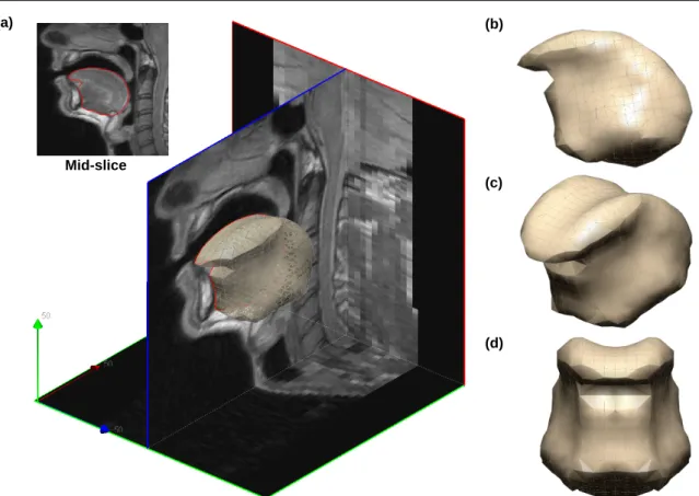
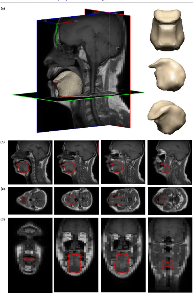
An atlas FE tongue mesh, which was previously elaborated by our group [58], has been employed to generate tongue FE meshes (for two patients and two healthy volunteers). The atlas-mesh was designed on the basis of 3D MR images of the vocal tract of a male subject, collected and segmented in the context of another study aiming at investigating the organization of articulatory configurations in the vocal tract during speech production [59]. After building a surface mesh from the segmented images, the FE tongue mesh was automatically generated using a method that optimizes the process in terms of elements quantity and quality, following preceding studies [8, 60, 61]. The atlas mesh is composed of 2180 nodes, and forming 3172 elements: 796 tetrahedrals, 766 pyramids, 432 wedges, and 1178 hexahedra. Fig. 3 shows the atlas MR image(of 25 saggital slices with a 256×256 scan matrix and voxel dimensions of 1×1×4mm)
superimposed with the tongue FE mesh.
Volume Image Registration
To extract a transformation that provides an accurate match between atlas and subject volumetric images, a two-level 3D image registration is used. First, a global transformation is calculated to provide an initial Rigid/Affine alignment. Then, a nonrigid method is used to establish the voxel-wise correspondence between the two volumes. As said above, based on preceding studies on Mesh-Match-and-Repair algorithm [15], the morphing algorithm should be continuously differentiable, non-folding and invertible. In other words, the transformation model should be a smooth bijective (one-to-one) mapping with a smooth inverse.
There are two popular non-rigid diffeomorphic registration methods: (1) Free-Form Deformations (FFDs), which are modeled by B-splines [25], and (2) the diffeomorphic Demons, which is a nonparametric diffeomorphic registration method based on Thirion’s demons algorithm [26]. Generally, the FFDs based registration algorithms are controlled by the underlying interpolation function, which provides more regular displacement fields than Demons-based approaches. Our group previously employed FFDs based algorithms. In this paper, the same FFD based method is chosen as the basis for the transformation model, which inherently generates smooth deformations. In addition, this model has been
reformulated using discrete Markov Random Fields (MRF) [27]. This amendment eliminates the procedure of customiz-ing the optimization method for different similarity measures in multi-modal volumetric image registration, which is a challenging problem in medical imaging [28]. In the next sections, the explanations of the diffeomorphic FFDs, their implementation and the employed optimization method in the subject-specific FE mesh generation process, are provided.
Free-Form Deformations
Non-rigid registration algorithms based on FFDs map each voxel of the atlas image into the corresponding voxel in the subject image using a deformation field that is optimally computed. The basic idea of these methods is to charac-terize deformations based on a grid of control points that are uniformly distributed throughout the fixed image’s voxel grid (herein the subject image). These control points partition the volume into equally sized regions (called tiles). The transformation model is a multilevel formulation of a FFDs based on tensor product of B-splines. B-splines enable inter-polating the dense deformation field from a given set of control points. Let us denote the domain of the image volume as
Ω ={(x, y, z)|0 ≤ x < X, 0 ≤ y < Y, 0 ≤ z < Z}. Let G denote a virtual deformable grid with spacings δx, δy, δz,
which is superimposed on the image volume. The nonlinear displacement field D is computed for each image point x = (x, y, z)by B-spline interpolation of the displacements of the grid control points:
D(x) = 3 ∑ l=0 3 ∑ m=0 3 ∑ n=0 Bl(u)Bm(v)Bn(w)di+l,j+m,k+n, (1)
where, i, j, and k denote the coordinates of the tile containing image point x and u, v, and w are the local coordinates of (x, y, z) within its housing tile: i =⌊x/δx⌋, j = ⌊y/δy⌋, k = ⌊z/δz⌋, u = x/δx− ⌊x/δx⌋, v = y/δy− ⌊y/δy⌋,
w = z/δz− ⌊z/δz⌋ (⌊ ⌋ is rounding operation). Blrepresents the lth basis function of the B-spline interpolation and
the displacement of the grid control points are denoted by d. So, di+l,j+m,k+nis the spline coefficient defining the
displacement for one of the 64 control points that influence the image point x within tile (i, j, k). Indeed, the B-splines serve as a weighted averaging function for the set of control points. Finally, the transformation of image point x can be computed by
T (x) = x + D(x) (2)
Given the source (J) and target (I) volumes, one seeks the optimal transformation by posing an energy minimization problem where the objective function is defined by a matching criterion S:
b
T = arg min
T S(I, J◦ T ) (3)
According to the application at hand, the matching criterion S may be Sum of Absolute/Squared Differences (SAD/SSD), Normalized Mutual Information (NMI) [29], Normalized Correlation Coefficient (NCC), Correlation Ratio (CR) [30], and etc.
The performance of registration methods based on FFDs is limited by the resolution of the control point grid, which generally determines the degrees of freedom and is linearly related to the computational complexity [25]:
– A coarse control point spacing enables modeling global and intrinsically smooth deformations.
– A finer control point spacing enables modeling more localized and intrinsically less smooth deformations.
Therefore, to refine the deformation field, a multi-level FFD is used to cover a wide range of transformations. The algorithm starts from a coarser control point spacing; when the algorithm reaches its optimal state, the control point spacing is reduced by a factor of two (in each dimension) to generate a finer grid. Also, for each level of control point spacing, several optimization cycles are performed to model a large deformation. Within each cycle of optimization process, an elementary transformation field is generated and the overall transformation can be computed as below:
T (x) = GJ z }| { TNJ J ◦ · · · ◦ T 1 J◦ · · · ◦ G1 z }| { TN1 1 ◦ · · · ◦ T 1 1, (4)
where Gj, j = 1,· · · , J are successive grid refinements, and Tji, i = 1,· · · , Nj are elementary deformations which
have been generated during each optimization cycle at grid level j.It should be noted that the initial control point spac-ing in the FFDs should be determined accordspac-ing to the application at the hand. As has been investigated in [27], when there is a good global correspondence between the volumes (provided by Rigid/Affine registration), employing an initial spacing of 20mm can capture the geometric structures accurately. However, a very coarse control point spacing enables FFDs to recover the Affine transformations [27].
As the FFDs are modeled by B-splines, the transformation model inherently satisfies the C1-differentiability. In order to preserve the bijectivity of the transformation, each elementary transformation is estimated by restricting the displace-ment of control points to 0.4 times the current control point spacing [25]. Since the overall transformation is computed by the combination of the elementary ones, it will be likewise a diffeomorphism. Although the regularity properties of the elementary registrations, namely non-folding and bijection, are enforced by restricting the amplitude of the displacement of the control points, it should be noted that the non-folding property is fulfilled locally at every point. Accordingly, the image-derived displacement fields may lead to unrealistic deformations and the deformed mesh may finally be prone to folding, as the consequence of crisscrossing of neighboring control points [31]. Therefore, an additional regularization term, which reduces mesh distortion, is considered as below:
R(T ) = ∑
p∈G
∑
q∈N(p)
| dp− dq|2, (5)
where dp is the displacement of the control point p in the virtual deformable grid G, and N (p) is the set of control
points which are located in the neighborhood of p, and defines the edges between p and others points in the control grid. This regularization term, which enforces a smooth transformation, leads neighboring control points to move in the same direction. Hence, the total cost function optimized in the registration problem is defined as the sum of two terms: a matching criterion (S) which quantifies the level of alignment between the two image volumes, and a regularization term (R) which imposes a smoothness constraint. The optimal transformation can be determined by posing an energy minimization problem where the objective function is a weighted sum of S and R:
b
T = arg min
where λ parameter acts as a weighting factor, controlling the influence of the regularization term. To obtain deformation parameters, a wide range of optimization strategies can be employed, including gradient descent [32], Newtons method [33, 34] , Powells method [35], and discrete optimization [36]. However, since the atlas and subject medical images can come from different modalities (e.g. CT or MRI), the possibility of using different similarity measures should be con-sidered. In that case, the optimization process will be dependent on the type of cost function and should be customized based on the employed one. This is why a discrete optimization strategy which is computationally efficient and also robust with respect to local optima, has been selected, namely the Markov Random Fields (MRF)-based optimization [28].
MRF-based Optimization
To obtain the deformation parameters, a numerical method has to be used to optimize the objective function in Eq. 6. For all the reasons mentioned in the previous section, a discrete optimization is used [28]. Broadly speaking, this projects the objective function back to the level of the control points, in order to transform it into a function of control points displacements instead of voxels displacements. Then, the displacement space is sampled in a discrete manner and the quantized displacement vectors are associated with labels, so that the optimization problem is converted to what is called “a labeling problem”. Finally, the appropriate optimization technique can be employed to extract a group of displacement vectors that collectively optimize the objective function. In this section, the employed discrete optimization strategy, from the conversion of the optimization problem to a labeling problem up to finding the best combination of labels or displacement fields, is briefly explained. For more details, the reader is referred to [27, 28].
The primary task is the reformulation of the optimization problem (Eq. 6) into a multi-labeling problem that can be expressed using first-order Markov Random Fields (MRFs) [37, 38]. Generally, a “labeling problem” consists of a set of objects to be classified, and a set of classes or labels. The objective of such a problem is to assign a label to each object, in a way that is consistent with some observed data that may contain pairwise relationships among the objects to be classified [38–40]. Markov random fields are used to model the statistical properties in the framework of probability theory. In the MRFs model, the probability of an object to belong to a specific class stands not only on its own feature but also on the labels of its neighboring objects. These objects can be considered as random variables whose values stand by the outcome of probabilistic experiments. Therefore, from the perceptive of MRFs, a labeling problem is defined in terms of a set of random variables and a set of labels that can be interpreted as events that can be happen to the random variables [38]. Consequently, at first, the role of the random variables and the definition of a discrete label space should be characterized. Considering the registration problem, a random variable is associated with every control point, and “labels” are defined corresponding to the displacements of the control points. Therefore, the continuous displacement space of the control points is quantized to generate a discrete set of displacement vectors Θ ={d1, ..., di}, and each
displacement vector is associated with a label (L ={l1, ..., li}). Also, assigning a label (lp) to a control point (p) is
equivalent to applying the displacement vector dlp to the control point p. In this study, the displacements along the
coordinate axes are sparsely sampled by a factor of n, from the minimum displacement to the maximum value (i.e., from zero to 0.4 times the current control point spacing [25]), which ends up having 6n+1 labels (displacements along
the six main axes plus the zero-displacement vector are considered). The problem can then be reformulated using the energy of first-order MRFs, which consists of sums of unary and pairwise potential functions:
EM RF(l) = ∑ p∈G Vp(lp) + λ ∑ p∈G ∑ q∈N(p) Vpq(lp, lq), (7)
where l is the labeling that we are looking for, Vp(.) is a unary potential function that corresponds to the energy
of assigning a label to the control point p, independently of all other control points [38]. As mentioned before, the labels are associated with the control points displacements. So, the unary potential term summed over all the control points encodes the matching criterion (S) in Eq. 6. Vpq(.) is a pairwise potential function that evaluates the consistency
between the labels of neighboring control points. In other words, it measures the cost of assigning displacements to the neighboring control points p and q. Therefore, the pairwise potential term summed over all the neighboring control points corresponds to the regularization term (R) in Eq. 6. The other two parameters N (p) and λ respectively define the control points neighboring region and control the influence of the regularization term. It is now important to note that, the matching criterion (S) in the energy optimization problem (Eq. 6) is defined on the image level. This criterion should therefore be projected back to the control points level using a weighting function so that the energy optimization problem could be mathematically reformulated using MRFs:
bη(|x − p|) = ∑η(|x − p|) y∈ Ω
η(|y − p|), (8)
wherebη(.) quantifies the impact of an image pixel x to a control point p, while η(.), quantifies the influence of a control point p to an image pixel x. The amount of influence is related to the distance between the image pixel x and the control point p; the farther they are, the less is the influence, and vice versa. Herein, the η(.) function is the B-spline function used in Eq. 1, that can be interpreted as a weighting function. Therefore, the unary potential function in the energy of MRF (in iteration t) can be rewritten as:
Vp(lp) =
∑ x∈ Ω
b
η(|x − p|) . S(I(x), J(Tt−1(x) + dlp)), (9)
where Tt−1is the overall transformation from the previous iteration and dlp is the next elementary displacement of
control point p. Accordingly, the unary potential at control point p is defined as the weighted combination of the data cost of those pixels that have an impact on the control point p. However, as previously mentioned, the unary potential function is assumed to be independent of all other control points. So, the unary potential is computed approximately under two simplifications [27]. First, the elementary displacement of each image point x (i.e., Eq. 1) is computed by direct translation of dlp(the displacement of control point p), instead of doing the interpolation between the displacement
of the neighboring control points. Second, with the aim to decrease the approximation error, the overlapping area for each control point is reduced by replacing the B-spline weighting functions inbη(.) (Eq. 8) with the linear ones. It should be reminded that B-spline functions are still kept to generate smooth transformation.
considered in the pairwise potential function as below:
Vpq(lp, lq) =| (R(p) + dlp)− (R(q) + dlq)|, (10)
whereR(.) projects the current overall transformation or displacement fields on the level of the control points as:
R(p) = ∑ x∈ Ω
bη(|x − p|)D(x) (11)
Thus, the registration problem is converted to a discrete labeling problem in the form of MRFs, and various optimization strategies can be applied to find the registration parameters. An efficient algorithm called FastPD is used in this study (for a full explanation of this method the reader is referred to [28]). To get accurate registration results, some param-eters controlling the discretization of the solution space have to be set. The first parameter is the maximum value of displacement which has been set to 0.4 times the current control point spacing [25]. As mentioned before, to refine the deformation field, a multi-level FFD is employed to cover a wide range of transformations; also, for each level of control point spacing, several optimization cycles (the second parameter, O) are performed to model a large deformation. How-ever, as FastPD generates quasi-optimal labelings on the discrete set of labels [27], it should be noticed that keeping the initial displacement set does not bring any further improvement. Therefore, each optimization cycle is done using a new set of displacement vectors. In this way, the initial maximum value of displacement is reduced by a scaling factor (the third parameter, α), and the new range has been re-sampled using the same method (with a specific number of steps, the fourth parameter, n). For the results provided later, the parameters are set to O = 5, α = 0.67 and n = 5 [27].
Mesh Morphing
The atlas-to-subject volumetric image registration provides a pair of transformations that establishes a one-to-one corre-spondence between the two volumes (atlas J and subject I). The first one is a Rigid/Affine transformation (TRigid/Affine)
that approximates the global transform between the two volumes, whereas the second one is a nonrigid transformation (TNonrigid) that locally refines the deformations from the Atlas to the subject. The next step towards atlas-mesh morphing
consists in defining the total transformation by combining the rigid and non-rigid transformations:
TTotal= TNonrigid◦ TRigid/Affine (12)
Depending on the type of atlas FE mesh that might be linear or non-linear, different methods of mesh morphing could be employed to generate subject-specific FE meshes from the 3D displacement fields [15, 14, 12, 18, 41, 42, 45]. In the case of linear FE meshes that nodes are defined by 2D or 3D coordinates and connected by straight lines or edges, the mesh morphing procedure could be summarized by simply moving the nodes along the dedicated displacement fields while keeping the previous connectivities. For each node, to approximate the new position, interpolation methods can be employed in order to provide the dedicated displacement fields (i.e., the interpolation of neighboring pixels displacements). In the case of non-linear meshes with higher order of interpolation (i.e., elements with higher-order
interpolation functions), appropriate techniques should be employed to find the projection of displacement fields into the basis functions of the mesh [46, 44, 43, 47–52]. However, as the proposed method is evaluated using a linear atlas FE mesh, each node of the atlas mesh is transformed by TTotalin order to generate the subject-specific mesh (with the same topology as for the atlas mesh since nodes connectivities are kept constant).
Evaluation
Image Registration Assessment
In order to quantitatively evaluate the performance of the inter-subject registration in capturing the geometric properties, the manual segmentation of the atlas and target organs are used. After doing the registration between the atlas and target images, the obtained transformations are employed to deform the atlas-binary mask onto the target images. Then, the Dice and volumetric overlap metrics, Hausdorff distance , and mean absolute surface are computed using the binary masks (i.e., the atlas-transformed masks and the reference segmentations). The Dice (D)and overlap fraction (O) are volumetric measures that compute the relative overlap of two binary masks. For each subject, the Dice and volumetric overlap of the atlas transformed mask (VAtlas-trans) and the reference segmentation (VManual) are respectively defined as
D(VAtlas-trans, VManual) =
2|VAtlas-trans∩ VManual| |VAtlas-trans| + |VManual|
(13)
O(VAtlas-trans, VManual) = |VAtlas-trans∩ VManual| |VAtlas-trans∪ VManual|
(14)
Both D and O values range from zero to one. A value close to one is desirable and means that there is a perfect match between the volumes, whereas a low value indicates a poor agreement. However, it should be noted that, both volumetric measures depend on the size and shape complexity of the objects and also are related to the volume sampling. So, in the case of large objects (e.g., Lung), they would be less sensitive to the small local errors that may exist on the boundaries. Therefore, Hausdorff (H) distance is also considered as an evaluation criteria to judge if the surfaces are close enough. Given two surfaces SAtlas-transand SManual, Hausdorff distance is defined as
H(SAtlas-trans, SManual) = max(h(SAtlas-trans, SManual), h(SManual, SAtlas-trans)) (15)
where
h(SAtlas-trans, SManual) = max
p∈SManual
(dmin(p, SManual)), (16) h(SManual, SAtlas-trans) = max
p∈SAtlas-trans
h(SAtlas-trans, SManual) measures the largest minimum distance from all points p on the surface SAtlas-transto the surface SManual, and vise versa for h(SManual, SAtlas-trans). Although Hausdorff distance is a useful measurement, it is overly sensitive to outliers. Even a single outlier can dominate the Hausdorff distance calculation, and leads to misleading results. However, it can provide useful information in conjunction with other metrics such as mean absolute surface distance (M), which is based on the Hausdorff distance and is defined as
M(SAtlas-trans, SManual) =
dmin(SAtlas-trans, SManual) + dmin(SManual, SAtlas-trans)
2 (18)
where dmin(SAtlas-trans, SManual) is the average minimum distance from all points on the surface SAtlas-trans) to the surface SManual), and vise versa for dmin(SManual, SAtlas-trans). Generally, mean absolute surface distance (M) indicates how much on average the two surfaces differ.
Mesh Quality Assessment
The regularity and quality of the deformed meshes are evaluated based on the Jacobian matrix [53]. The Jacobian matrix is the fundamental quantity describing all the first-order mesh qualities (length, areas and angles) of interest [53]. The regularity assessment is function of the Jacobian matrix determinant (detJ, also called theJacobian) and evaluates whether the employed FE mesh can be used for numerical analysis. TheJacobian must be checked for all the elements of the FE mesh as it is influenced by the configuration of the element nodes. Within each element, the Jacobian is computed for each node, and the element (and subsequently the FE mesh) is classified irregular if one of the nodes has a zero or negative value. It is worth pointing out that theJacobian value measures the distortion of the actual mesh element with respect to its reference configuration, but not the overall distortion information. To deal with this problem, the quality of each element can be determined at the level of its nodes (e.g., node n) by a ratio of nodalJacobian value to the maximalJacobian value among those computed at all element nodes (thus interpreted as a global distortion information). Such a ratio measures the node quality within its element (e) and is called Jacobian Ratio (JR) [53]:
JR JR JRen= detJJJ(n) max n∈e {detJJJ(n)} (19)
The JR values range from zero to one. Having a high value (close to one) for JRJRJRenmeans that the element (e) has a
high quality at node n, whereas a low value (close to zero) indicates a poor quality at node n. To evaluate the quality of each element, the JR is computed for all the element nodes and the minimum value is returned as an indicator of element quality (JRemin). In the ideal state, all elements of a given mesh are expected to have high JR values; however
in many cases this is impossible. That is why, for example, the commercial FE analysis software ANSYS sets a minimal value of 0.03 for JR [54].
RESULTS
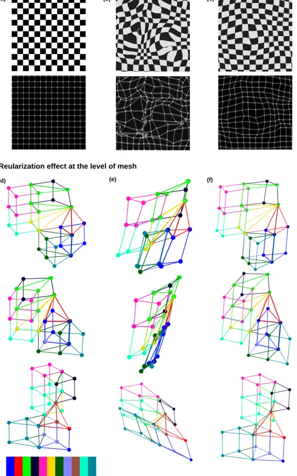
Before showing the results of mesh generation, it is important to illustrate how efficiently the regularization term pre-vents the introduction of foldings in the deformed meshes. In this respect, Fig. 4 shows the results of applying two transformations that are obtained without and with the regularization term. The same evaluation is also done at the level of mesh structure formation. To have a clear understanding, only a section of the atlas tongue mesh (including 11 ele-ments) is selected and depicted. As can be seen, the level of mesh distortions is dramatically reduced by virtue of the regularization term. These two examples illustrate how the regularity and quality of the meshes can be preserved thanks to the diffeomorphic constraints and the regularization term. It should be noted that the effect of the regularization term, which can be interpreted as a smoothness term, is controlled by the weighting factor λ (in Eq. 6). The value of λ has to be set according to the application and to the type of the employed similarity measure. Generally, a higher value of λ provides a smoother deformation thus less quality degradation. It is important however to note that sharp morphological structures are modeled less accurately using a large weighting factor.However, it may raise the question that how accu-rately geometric properties are captured under these constraints. To answer this principle question, before showing the results of mesh quality assessment, the same registration strategy is applied to a data set of chest CT scans that includes Lung manual segmentations.
Chest CT Image Registration
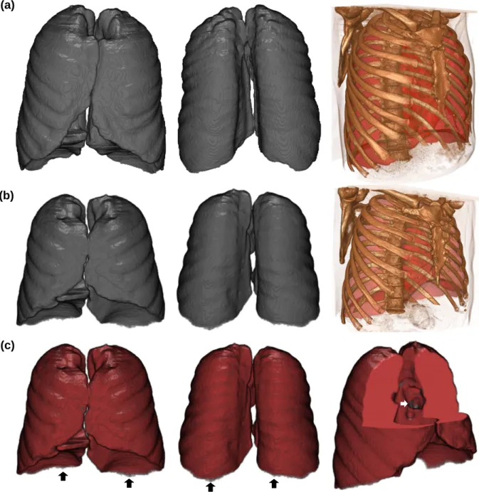
Image-registration-based subject-specific Lung masks are generated for 12 healthy and diseased subjects. After extrac-tion of deformaextrac-tions from the atlas CT image, the atlas-binary mask is deformed onto the target images. As the Lung is a big object, the non-rigid registration is applied in two levels. First, the SAD (Sum of Absolute Differences) simi-larity measure with a big value of λ (i.e., regularization weight) is employed in order to capture the principle geometric properties of the target Lung (with a very coarse initial control point spacing of 60 mm). Then, for small details of the shape, the similarity measure is changed into SSD (Sum of Squared Differences) and λ is also decreased (with an initial control point spacing of 25mm). The evaluation of the results performed qualitatively and quantitatively as follows. Fig. 5, shows the result of Lung CT image registration for a typical CT scan. Manual Lung segmentation in the atlas CT-image, and manual Lung segmentation of the target CT-image are respectively shown in Fig. 5(a) and (b). Finally, atlas-driven subject-specific Lung mask is superimposed on the manual segmentation in the Fig. 5(c). As it is seen, there is a good correlation between the atlas-driven subject-specific Lung mask and the reference one indicating the acceptable performance of the suggested algorithm. However, the sharp regions, specially at the bottom of the Lung, are captured less accurately. In quantitative evaluation step, the Dice (D), overlap fraction (O), Hausdorff distance (H), and mean absolute surface (M) are calculated for all subjects. Mean and standard deviation (SD) are computed for the mentioned metrics as follows (in mm): D = 0.98± 0.01, O = 0.96 ± 0.01, H = 34.25 ± 7.75, and M = 0.98 ± 0.26. The quantitative results show that the performance of the mesh quality preserved registration method is good enough to capture the target organs; however, high values of H were expected (because of the outliers).
FE tongue meshes generation
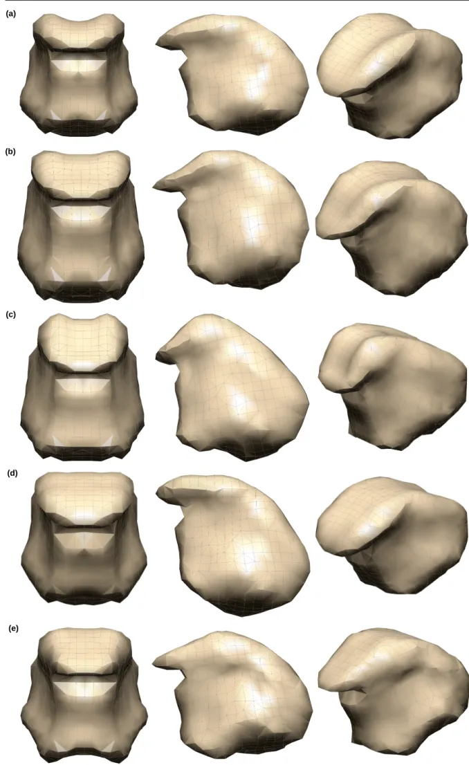
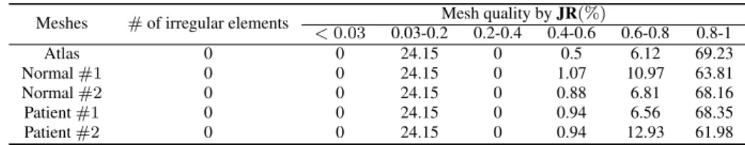
The generated subject-specific tongue FE meshes are shown in Fig. 6. The data set includes two healthy subjects and two patients suffering tongue cancer. The regularity and quality of generated meshes are assessed using Jacobian Ratio (JR). In this matter, as explained in the preceding section, the Jacobian Ratio of each element (JRemin) is calculated and the
mean value of all elements qualities is reported as the quality indicator of the mesh. This assessment is presented in Table 1. All generated meshes contain no irregular element (JR < 0). To have a more detailed assessment as concerns mesh quality, the elements are classified into six Jacobian Ratio categories. Elements with JR value between zero and 0.03 are considered as poor quality elements. As can be seen, none of the generated meshes includes poor quality element, indicating that the proposed method can be considered as a promising strategy to generate subject-specific FE meshes while keeping the regularity and quality of the elements.
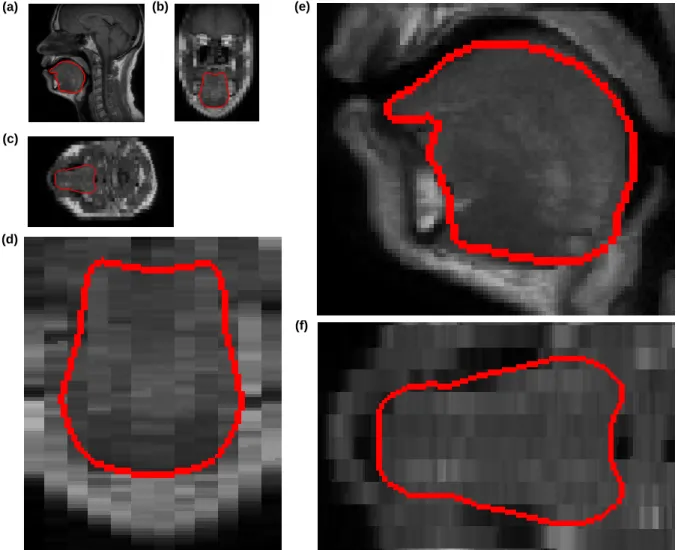
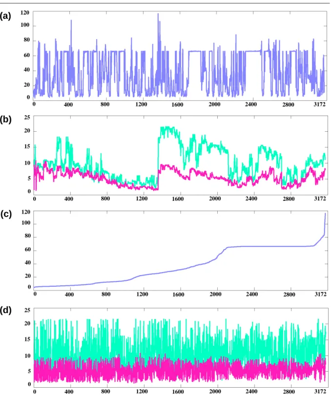
Finally, Fig. 7 focuses on one of the two volunteers for whom the MRI exam was of 32 slices with a 1mm× 1mm pixels size and 5mm inter-slice distance. The external contours of the generated FE mesh is superimposed with Sagittal and Coronal slices extracted from this MR exam.Also, the enlarged tongue regions for some slices are provided in Fig. 8. In addition, elements-size-distribution for the atlas FE tongue mesh and their maximum nodal displacements (in mm), after employing the proposed approach and pure non-rigid registration (i.e., without constraints), are shown in Fig. 9. Volumes of all elements are computed and plotted in Fig. 9(a), according to their element-order within the original file. Fig. 9(b) shows the maximum nodal displacements (in mm) for all elements. As it is seen, there are some big variations in the displacements, depicting that subsequent elements are located in another region of the tongue which may have more-or-less transformations. In Fig. 9(c), the elements-size-distribution is again depicted, however, the elements are sorted according to their size; and their displacements are displaced in Fig. 9(d). It is clear that the displacements are controlled by the employed constraints.
Qualitative evaluation with a patient-specific tongue model
For one of the patients (Patient #2) , activation of the posterior genio-glossus (GGp) muscle (one of the most important muscles of the tongue) is simulated before and after surgery. This muscle is located at the root of the tongue and its activation propels the tongue frontwards and upwards in its front part. Its role in speech production is crucial since it is strongly involved in the production of the phonemes /i/ and /s/. Muscle activation is modeled using the FE formulation of the Hill muscle model proposed by [62], which includes both the active stress stiffening effect and the passive transversal isotropy of muscles [63]. For the passive response, we used a simplified 5-parameter Mooney-Rivlin hyperelastic model with constitutive parameters derived from previous work [58]. The assignment of the muscle fiber direction in each element of each muscle group in the tongue mesh is performed automatically based on the fibers direction extracted for the atlas mesh in a previous work in our team [60] from the Visible Human Project dataset. Tongue cancer surgery is accounted for in the model by modifying the biomechanical properties of the tongue tissues that are planned to be excised and reconstructed during a hemi-glossectomy procedure (half of the upper tongue is removed and replaced with a flap). In the model, the active material properties of the GGp elements that are removed
and reconstructed are then replaced with passive material properties. Fixed boundary conditions are enforced on the bottom nodes of the model to simulate very roughly the role of the mouth floor and the attachments to the mandible. Fig. 10 plots the response of the tongue model to the activation of the GGp before and after the hemi-glossectomy. Both the distribution of the Von mises equivalent strain in the GGp muscle and the displacement of the tongue are provided.
DISCUSSION
In this paper a novel methodology, for automatic subject-specific FE mesh generation, is proposed. Contrary to the previous efforts in the literature, which need typical-information extraction, employing meshing algorithms or refine-ment post-processing steps (e.g., for mesh quality improverefine-ment), the proposed method does not require extraction of prior-knowledge on the shape of the target-organ, and subsequently, no meshing algorithm. As the main objective of this research is to develop a non-prior knowledge dependent method that is compatible with the times of the clinical practice, image-based registration methods are employed to deform an atlas FE mesh and to automatically generate subject-specific meshes.
To evaluate the performance of the proposed method, FE subject-specific tongue meshes were generated. Fig. 6 il-lustrates well the capacity of the method to generate various kinds of speaker-specific tongue anatomy at rest. These differences can be due to strong differences in global vocal tract anatomy (see for example differences between Pa-tient #2 (e) and Atlas) or to muscle activations at rest (see for example differences between PaPa-tient #1 (d) and Atlas). From a more quantitative point of view, the quality assessments reveal that the regularity and quality of the meshes are preserved. Contrary to Mesh-Morphing methods that sometimes need to post-process the mesh because of irregular ele-ments ([20]), we observe in our results that all generated meshes are regular and can be used for FE analysis. Moreover, the quality of the mesh is almost maintained. Indeed, the percentage of elements within the quality range of 0.8− 1 is slightly decreased by less than 8% (table 1). This small reduction in the number of high quality elements results in small increment in the lower quality ranges (maximally 6.81% and 0.57% for the ranges of 0.6− 8 and 0.4 − 0.6, respectively).
Fig. 7 plots the contours of one generated mesh superimposed with the corresponding MR slices. The various slices displayed in the figure illustrate the efficiency of the method since the contours fit well with the observed boundaries of tongue tissues. Moreover, for some slices for which it is quite difficult to see tongue contours (the lateral sagittal views close to cheeks tissues or tongue basement), we can note that our registration method is able to suggest tongue contours thus maintaining a coherent structure for the whole 3D mesh.
Focusing on one of the two patients, we have proposed to simulate some functional consequences of a surgical gesture. Whereas the relevance of such use of a biomechanical model for computer assisted surgery has already been provided ([64]), the objective here was to propose an illustration of a tentative fully automatic procedure compatible with the clin-ical constraints. Therefore, starting from an MRI exam of a patient, we were able to automatclin-ically generate an FE model of that patient. All the information included in the tongue atlas model was automatically transferred in the model of the patient. It was thus straightforward to simulate the activation of the posterior genioglossus muscle. The corresponding results provided by Fig. 10 confirm a clinical observation, namely the fact that, after a hemi-glossectomy, the tongue
response is no more symmetric. This is obviously due to the non-symmetric activation pattern of the GGp muscle. The results also predict that the patient might have difficulties to move its tongue in the front and upper part of the oral cavity since the simulated displacements after surgery are significantly lower than the ones simulated before hemiglossectomy. The atlas-based subject-specific FE model generation method proposed in this paper seems to provide efficient results that were qualitatively and quantitatively evaluated on four subjects. Tongue models were used here since it is a clini-cal case for which the manual delineation of tongue contours is a particularly complex and sometimes impossible task ([57]). The counterpart of this choice is that it is impossible to design a gold standard case to which we could compare the results proposed by our method. Indeed, since boundaries are difficult to identify for some regions of the tongue (e.g. at the bottom and laterally), we were not able to ask an expert to segment a whole tongue and to guaranty that this segmentation would be considered as the gold standard.
Considering the results of the chest CT registration, in order to capture the sharp or fine structures, that may not exist in the atlas or subject’s image, applying another registration step with less strong constraints might be useful. An-other idea that might be of interest would be employing an additional registration step that is free of any mesh quality preservation constraints. In other words, it can be assumed that the proposed approach provides a high quality pre-final subject-specific FE mesh that is, probably, the most similar one to the target organ. At the next step, to generate the final subject-specific FE mesh, deformations of the surface nodes, that are extracted from the last registration step (free of constraints), can be distributed to whole nodes inside. However, these possible solutions need to be examined to ensure that the quality of the deformed FE mesh is preserved.Finally, it should be noted that our method still needs to define the weighting factor lambda that controls the influence of the regularization term. This highly depends on the image modality as well as the type of organ. Our method needs therefore definitively to be more extensively evaluated on a larger set of tongue MR images.
Acknowledgements This work was partly funded by the AGIR program (Grenoble Universities) and by the ANR under reference ANR-11-LABX-0004. We are grateful to Georges Bettega (Grenoble Hospital), Mayra Moya Espinosa (Ensam Paris), Chenchen Tong (National University of Singapore) and Marek Bucki (Texisense Company) for many interactions and inputs to this study.
References
1. Weatherill, N. P., and O. Hassan. Efficient three?dimensional Delaunay triangulation with automatic point creation and imposed boundary constraints. International Journal for Numerical Methods in Engineering. 12: 2005-2039, 1994.
2. Molino, N., R. Bridson, J. Teran, and R. Fedkiw. A Crystalline, Red Green Strategy for Meshing Highly Deformable Objects with Tetrahe-dra. In 12th International Meshing Roundtable, Santa Fe, New Mexico, USA. 103-114, 2003.
3. Fang, Q., and D. A. Boas. Tetrahedral mesh generation from volumetric binary and gray-scale images. In: ISBI’09 Proceedings of the 6th IEEE International Conference on Symposium on Biomedical Imaging: From Nano to Macro, Boston, MA. 1142-1145, 2009.
4. Mohamed, A., and C. Davatzikos. Finite element mesh generation and remeshing from segmented medical images. In: ISBI’04 Proceedings of the 6th IEEE International Conference on Symposium on Biomedical Imaging: From Nano to Macro. 1: 420-423, 2004.
5. Zhang Y, Bajaj C, Sohn BS. 3D finite element meshing from imaging data, Computer Methods in Applied Mechanics and Engineering. 194(48): 5083-5106, 2005.
6. Zhang, Y., T. JR. Hughes, and C. L. Bajaj. Automatic 3D mesh generation for a domain with multiple materials. In Proceedings of the 16th international meshing roundtable, Springer Berlin Heidelberg. 367-386, 2008.
7. Lederman, C., A. Joshi, I. Dinov, L. Vese, A. Toga, and J. D. Van Horn. The generation of tetrahedral mesh models for neuroanatomical MRI, NeuroImage. 55(1): 153-164, 2011.
8. Rohan, P-Y., C. Lobos, M. A. Nazari, P. Perrier, and Y. Payan. Finite element modelling of nearly incompressible materials and volumetric locking: a case study. Computer methods in biomechanics and biomedical engineering. 17(sup1), 192-193, 2014.
9. Benzley, S. E., E. Perry, K. Merkley, B. Clark, and G. Sjaardama. A comparison of all hexagonal and all tetrahedral finite element meshes for elastic and elastoplastic analysis. In Proceedings, 4th International Meshing Roundtable. 17: 179-191, 1995.
10. Keyak, J. H., J. M. Meagher, H. B. Skinner, and C. D. Mote. Automated three-dimensional finite element modeling of bone: A new method. Journal of Biomedical Engineering. 12(5): 389-397, 1990.
11. Viceconti, M., M. Davinelli, F. Taddei, and A. Cappello. Automatic generation of accurate subject-specific bone finite element models to be used in clinical studies, Journal of Biomechanics. 37:1597-1605, 2004.
12. Couteau, B., Y. Payan, and S. Lavall´ee. The mesh-matching algorithm: an automatic 3D mesh generator for finite element structures. Journal of biomechanics. 33(8): 1005-1009, 2000.
13. Fernandez, J. W., P. Mithraratne, S. F. Thrupp, M. H. Tawhai, and P. J. Hunter. Anatomically based geometric modelling of the musculo-skeletal system and other organs. Biomechanics and modeling in mechanobiology. 2(3): 139-155, 2004.
14. Sigal, I. A., M. R. Hardisty, and C. M. Whyne. Mesh-morphing algorithms for specimen-specific finite element modeling. Journal of biomechanics, 41(7): 1381-1389, 2008.
15. Bucki, M. , C. Lobos, and Y. Payan. A fast and robust patient specific finite element mesh registration technique: application to 60 clinical cases. Medical image analysis. 14(3): 303-317, 2010.
16. Grassi, L., N. Hraiech, E. Schileo, M. Ansaloni, M. Rochette, and M. Viceconti. Evaluation of the generality and accuracy of a new mesh morphing procedure for the human femur. Medical engineering and physics. 33(1): 112-120, 2011.
17. Barber, D. C., E. Oubel, A. F. Frangi, and D. R. Hose. Efficient computational fluid dynamics mesh generation by image registration. Medical image analysis. 11(6): 648-662, 2007.
18. Lamata, P., S. Niederer, D. Nordsletten, D. C. Barber, I. Roy, D. R. Hose, and N. Smith. An accurate, fast and robust method to generate patient-specific cubic Hermite meshes. Medical image analysis. 15(6): 801-813, 2011.
19. Lamata, P., I. Roy, B. Blazevic, A. Crozier, S. Land, S. A. Niederer, D. Hose, and N. P. Smith. Quality metrics for high order meshes: analysis of the mechanical simulation of the heart beat. IEEE Transactions on Medical Imaging, 32(1): 130-138, 2013.
20. Bucki, M., C. Lobos, Y. Payan, and N. Hitschfeld. Jacobian-based repair method for finite element meshes after registration. Engineering with Computers. 27(3): 285-297, 2011.
21. Ji, S., J. C. Ford, R. M. Greenwald, J. G. Beckwith, K. D. Paulsen, L. A. Flashman, and T. W. McAllister. Automated subject-specific, hexahedral mesh generation via image registration. Finite Elements in Analysis and Design. 47(10): 1178-1185, 2011.
22. Chenchen, Tong. Generation of Patient-Specific Finite-Element Mesh from 3D Medical Images. Doctoral dissertation, National University of Singapore, 2013.
23. Murphy, K., B. Van Ginneken, J. M. Reinhardt, S. Kabus, K. Ding, X. Deng, K. Cao et al. Evaluation of registration methods on thoracic CT: the EMPIRE10 challenge. Medical Imaging, IEEE Transactions on 30, no. 11: 1901-1920, 2011.
24. Van Rikxoort, E. M., B. D. Hoop, M. A. Viergever, M. Prokop, and B. V. Ginneken. Automatic lung segmentation from thoracic computed tomography scans using a hybrid approach with error detection. Medical physics 36, no. 7: 2934-2947, 2009.
25. Rueckert, D., P. Aljabar, R. A. Heckemann, J. V. Hajnal, and A. Hammers. Diffeomorphic registration using B-splines. In Medical Image Computing and Computer-Assisted InterventionMICCAI, Springer Berlin Heidelberg. 702-709, 2006.
26. Vercauteren, T., X. Pennec, A. Perchant, and N. Ayache. Diffeomorphic demons: Efficient non-parametric image registration. NeuroImage. 45(1): S61-S72, 2009.
27. Glocker, B., N. Komodakis, G. Tziritas, N. Navab, and N. Paragios. Dense image registration through MRFs and efficient linear program-ming. Medical image analysis. 12(6): 731-741, 2008.
28. Komodakis, N., G. Tziritas, and N. Paragios. Fast, approximately optimal solutions for single and dynamic MRFs. IEEE Conference on Computer Vision and Pattern Recognition (CVPR’07). 1-8, 2007.
29. Maes, F., A. Collignon, D. Vandermeulen, G. Marchal, and P. Suetens. Multimodality image registration by maximization of mutual information. IEEE Transactions on Medical Imaging. 16(2): 187-198, 1997.
30. Roche, A., G. Malandain, X. Pennec, and N. Ayache. The correlation ratio as a new similarity measure for multimodal image registration. In Medical Image Computing and Computer-Assisted InterventationMICCAI, Springer Berlin Heidelberg. 1115-1124, 1998.
31. Brock, K. K. (Ed.). Image Processing in Radiation Therapy. CRC Press, 2013.
32. Rueckert, D., L. I. Sonoda, C. Hayes, D. LG Hill, M. O. Leach, and D. J. Hawkes. Non-rigid registration using free-form deformations: Application to breast MR images, IEEE Transactions on Image Processing. 18(8): 712-721, 1999.
33. Wright, S. J., and J. Nocedal. Numerical optimization. Vol. 2. New York: Springer, 1999.
34. Mattes, D., D. R. Haynor, H. Vesselle, T. K. Lewellen, and W. Eubank. PET-CT image registration in the chest using free-form deforma-tions. IEEE Transactions on Medical Imaging. 22(1), 120-128, 2003.
35. Powell, M. JD. A fast algorithm for nonlinearly constrained optimization calculations. In Numerical analysis, Springer Berlin Heidelberg. 144-157, 1987.
36. K. Nikos, G. Tziritas, and N. Paragios. Performance vs computational efficiency for optimizing single and dynamic MRFs: Setting the state of the art with primal-dual strategies. Computer Vision and Image Understanding. 112(1): 14-29, 2008.
37. Geman, S., and D. Geman. Stochastic relaxation, Gibbs distributions, and the Bayesian restoration of images. IEEE Transactions on Pattern Analysis and Machine Intelligence. 6: 721-741, 1984.
38. Li, S. Z. Markov random field modeling in image analysis. Springer Science Business Media, 2009. 39. Breiman, L., J. Friedman, C. J. Stone, and R. A. Olshen. Classification and regression trees. CRC press, 1984. 40. Ditterrich, T. G. Machine learning research: four current direction. Artificial Intelligence Magzine. 4: 97-136, 1997.
41. Baldwin, M. A., J. E. Langenderfer, P. J. Rullkoetter, and P. J. Laz. Development of subject-specific and statistical shape models of the knee using an efficient segmentation and mesh-morphing approach. Computer methods and programs in biomedicine. 97(3): 232-240, 2010. 42. Bah, M. T., P. B. Nair, and M. Browne. Mesh morphing for finite element analysis of implant positioning in cementless total hip
replace-ments. Medical engineering & physics, 31(10): 1235-1243, 2009.
43. Reddy, J. N. An Introduction to Nonlinear Finite Element Analysis: with applications to heat transfer, fluid mechanics, and solid mechan-ics. OUP Oxford, 2014.
44. Sigal, I. A., & C. M. Whyne. Mesh morphing and response surface analysis: quantifying sensitivity of vertebral mechanical behavior. Annals of biomedical engineering, 38(1), 41-56, 2010.
45. Zhang, S., Y. Zhan, X. Cui, M. Gao, J. Huang, & D. Metaxas. 3D anatomical shape atlas construction using mesh quality preserved deformable models. Computer Vision and Image Understanding, 117(9): 1061-1071, 2013.
46. Alexa, M.: Recent advances in mesh morphing. In Computer graphics forum (Vol. 21, No. 2, pp. 173-198). Blackwell Publishers Ltd., June 2002.
47. Helenbrook, B.T. Mesh deformation using the biharmonic operator. Int. J. Num. Meth. Engr. 56: 10071021, 2003.
48. Shontz, S.M., S.A. Vavasis. A mesh warping algorithm based on weighted Laplacian smoothing. In: Proc. 12th Int. Meshing Roundtable. 147158, 2003.
49. Shontz, S.M., & S.A. Vavasis. Analysis of and workarounds for element reversal for a finite element-based algorithm for warping triangular and tetrahedral meshes. BIT, Numerical Mathematics 50, 863884, 2010.
50. Stein, K., T. Tezduyar, R. Benney. Mesh moving techniques for fluid-structure interactions with large displacements. Trans. ASME 2003, 70: 5863, 2003.
51. Michler, A.K. Aircraft control surface deflection using RBF-based mesh deformation. Int. J. Num. Meth. Engr., doi: 10.1002/nme.3208, 2011.
52. Staten, M. L., S. J. Owen, S. M. Shontz, A. G. Salinger, & T. S. Coffey. A comparison of mesh morphing methods for 3D shape optimiza-tion. In Proceedings of the 20th international meshing roundtable, Springer Berlin Heidelberg. 293-311, 2012.
53. Knupp, P. M. Achieving finite element mesh quality via optimization of the Jacobian matrix norm and associated quantities. Part IIa framework for volume mesh optimization and the condition number of the Jacobian matrix. International Journal for numerical methods in engineering. 48(8): 1165-1185, 2000.
54. Kelly S, Element shape testing, in: Ansys Theory Reference, Chap 13, Ansys, USA, 1998. 55. Iskarous, K. Patterns of tongue movement. Journal of Phonetics, 33(4), 363-381, 2005.
56. Lee, J., J. Woo, F. Xing, E. Z. Murano, M. Stone, and J. L. Prince. Semi-automatic segmentation for 3D motion analysis of the tongue with dynamic MRI. Computerized Medical Imaging and Graphics. 38(8): 714-724, 2014.
57. M. Harandi, N., R. Abugharbieh, and S. Fels. 3D segmentation of the tongue in MRI: a minimally interactive model-based approach. Computer Methods in Biomechanics and Biomedical Engineering: Imaging & Visualization, no ahead-of-print. 1-11, 2014.
58. Buchaillard, S., P. Perrier, and Y. Payan. A biomechanical model of cardinal vowel production: Muscle activations and the impact of gravity on tongue positioning. The Journal of the Acoustical Society of America. 126(4): 2033-2051, 2009.
59. Badin, P., P. Borel, G. Bailly, L. Revret, M. Baciu, and C. Segebarth. Towards an audiovisual virtual talking head: 3D articulatory modeling of tongue, lips and face based on MRI and video images. In 5th Speech Production Seminar. 261-264, 2000.
60. Gerard, J.M., R. Wilhelms-Tricarico , P. Perrier, and Y. Payan. A 3D dynamical biomechanical tongue model to study speech motor control. Recent Research Developments in Biomechanics. 1: 49-64, 2003.
61. Lobos, C., Y. Payan, and N. Hitschfeld. Techniques for the generation of 3D Finite Element Meshes of human organs. In A. Daskalaki (Ed.), Informatics in Oral Medicine: Advanced Techniques in Clinical and Diagnostic Technologies. Hershey, PA: Medical Information Science Reference. 126-158, 2010.
62. Blemker, S. S., P. M. Pinsky, and S. L. Delp. A 3D model of muscle reveals the causes of nonuniform strains in the biceps brachii. Journal of biomechanics. 38(4): 657-665, 2005.
63. Nazari, M. A., P. Perrier, and Y. Payan. The Distributed Lambda (λ) Model (DLM): A 3-D, Finite-Element Muscle Model Based on Feldman’s λ Model; Assessment of Orofacial Gestures. Journal of speech, language, and hearing research. 56(6): 1909-1923, 2013. 64. Buchaillard, S., M. Brix, P. Perrier, and Y. Payan. Simulations of the consequences of tongue surgery on tongue mobility: implications for
speech production in post?surgery conditions. The International Journal of Medical Robotics and Computer Assisted Surgery. 3(3), 252-261, 2007.
List of Tables
Table 1.Table 1.Table 1. Mesh quality distribution for the atlas and subject FE tongue meshes generated by the proposed method.
List of Figures
Fig. 1.Fig. 1.Fig. 1. Block diagram of the Mesh-Match-and-Repair (MMRep) algorighm for generation of the 3D subject-specific FE meshes [15].
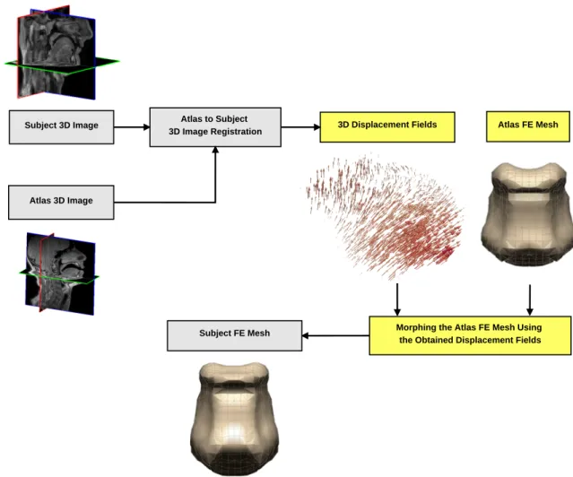
Fig. 2.Fig. 2.Fig. 2. General dataflow proposed to generate 3D subject-specific FE meshes.
Fig. 3.Fig. 3.Fig. 3. Atlas MR data superimposed with the 3D atlas FE tongue mesh, (b) Side, (c) isometric and (d) front views respectively of the 3D FE tongue mesh.
Fig. 4.Fig. 4.Fig. 4. Effect of the regularization term: at the level of the image, (a) input image and the distribution of control points, (b) deformed input image without using the regularization term and the distribution of control points after registration, (c) deformed input image in the presence of the regularization term and the distribution of control points after registration; and at the level of the mesh, (d) a section of the atlas FE Mesh, (e) deformed mesh without using the regularization term (f) deformed mesh using the regularization term (different views are provided in each row: side, front, and back, in order from top to bottom).
Fig. 5.Fig. 5.Fig. 5.Result of the Lung CT image registration: (a) Manual Lung segmentation in the atlas CT-image (at each column, from left to right: front view, back view, and 3D chest CT reconstruction embracing the Lung manual segmentation), (b) Manual Lung segmentation in a typical CT-image (at each column, from left to right: front view, back view, and 3D chest CT reconstruction embracing the Lung manual segmentation), (c) Atlas-driven subject-specific Lung, in Grey, superimposed on the manual segmentation, in Red (at each column, from left to right: front view, back view, and a cut-out to the region having less accuracy).
Fig. 6.Fig. 6.Fig. 6. Result of atlas FE mesh morphing using the proposed method: (a) Atlas FE tongue mesh (b) Subject-specific FE tongue mesh (Normal #1), (c) subject-specific FE tongue mesh (Normal #2), (d) Patient-specific FE tongue mesh (Patient #1), (e) Patient-specific FE tongue mesh (Patient #2).
Fig. 7.Fig. 7.Fig. 7. Mesh derived tongue contours superimposed on the MR image: (a) 3D subject-specific FE tongue mesh (Normal #1), (b) Sagittal views (mid-sagittal to the lateral side), (c) Axial views (inferior to superior), (d) Coronal views (anterior to posterior).
Fig. 8.Fig. 8.Fig. 8.Mesh derived tongue contours superimposed on the MR images and their enlargements (Normal #1) : (a) a Sagittal slice, (c) a Coronal slice, (d) an Axial slice, (d) enlargement of the tongue region in the Sagittal slice, (e) enlargement of the tongue region in the Coronal slice, (f) enlargement of the tongue region in the Axial slice.
Fig. 9.Fig. 9.Fig. 9.Representation of elements size in the atlas FE tongue mesh, and their displacements with and without constraints: (a) Elements-size-distribution for the atlas FE tongue mesh (in mm3), (b) Maximum nodal displacement (in mm), within each element, for two generated meshes: (1) Generated subject-specific FE mesh using the proposed approach, for Normal #2 (in violet), and (2) Generated subject-specific FE mesh using pure non-rigid registration (i.e., without constraints), for Normal #2 (in green), containing 58 irregular elements (JR < 0), (c) Volume of all elements, sorted
based on the element size, within the atlas FE tongue mesh (in mm3), (c) Elements-size-distribution for all elements, sorted by their size, (d) Maximum nodal displacement (in mm), within each element, for the same meshes (element-size ordered).
Fig. 10.Fig. 10.Fig. 10. Biomechanical response of the tongue model to the activation of the GGp before and after surgery: (a) Sagittal view of the tongue showing the implementation of the GGp, (b) Front view of the tongue before surgery , (c) Front view of the tongue after surgery; the right part of the muscle has been removed, (d) Distribution of the Von Mises equivalent strain in the GGp after its activation in pre-surgery condition, (e) Distribution of the Von Mises equivalent strain in the GGP after its activation in post-surgery condition, (f) Displacement map in the tongue after GGP activation in pre-surgery condition, (g) Displacement map in the tongue after GGP activation in post-surgery condition.
Meshes # of irregular elements Mesh quality by JR(%) < 0.03 0.03-0.2 0.2-0.4 0.4-0.6 0.6-0.8 0.8-1 Atlas 0 0 24.15 0 0.5 6.12 69.23 Normal #1 0 0 24.15 0 1.07 10.97 63.81 Normal #2 0 0 24.15 0 0.88 6.81 68.16 Patient #1 0 0 24.15 0 0.94 6.56 68.35 Patient #2 0 0 24.15 0 0.94 12.93 61.98
Region-of-Interest (ROI)
Segmentation Surface Creation Subject 3D image
Mesh-Match-and-Repair (MMRep) Subject FE Mesh
Atlas FE Mesh
Subject 3D Image
Atlas 3D Image
Atlas to Subject
3D Image Registration Atlas FE Mesh
Morphing the Atlas FE Mesh Using the Obtained Displacement Fields Subject FE Mesh
3D Displacement Fields
(a) (b)
(c)
(d) Mid-slice
Fig. 3 (a) Atlas MR data superimposed with the 3D atlas FE tongue mesh, (b) Side, (c) isometric and (d) front views respectively of the 3D FE tongue mesh.
(b)
(a) (c)
(f)
(d) (e)
Reularization effect at the level of image
Reularization effect at the level of mesh
Fig. 4 Effect of the regularization term: at the level of the image, (a) input image and the distribution of control points, (b) deformed input image without using the regularization term and the distribution of control points after registration, (c) deformed input image in the presence of the regularization term and the distribution of control points after registration; and at the level of the mesh, (d) a section of the atlas FE Mesh, (e) deformed mesh without using the regularization term (f) deformed mesh using the regularization term (different views are provided in each row: side, front, and back, in order from top to bottom).
(b)
(c)
(a)
Fig. 5 Result of the Lung CT image registration: (a) Manual Lung segmentation in the atlas CT-image (at each column, from left to right: front view, back view, and 3D chest CT reconstruction embracing the Lung manual segmentation), (b) Manual Lung segmentation in a typical CT-image (at each column, from left to right: front view, back view, and 3D chest CT reconstruction embracing the Lung manual segmentation), (c) Atlas-driven subject-specific Lung, in Grey, superimposed on the manual segmentation, in Red (at each column, from left to right: front view, back view, and a cut-out to the region having less accuracy).
(d) (b)
(c) (a)
(e)
Fig. 6 Result of atlas FE mesh morphing using the proposed method: (a) Atlas FE tongue mesh (b) Subject-specific FE tongue mesh (Normal #1), (c) subject-specific FE tongue mesh (Normal #2), (d) Patient-specific FE tongue mesh (Patient #1), (e) Patient-specific FE tongue mesh (Patient #2).
(a)
(b)
(c)
(d)
Fig. 7 Mesh derived tongue contours superimposed on the MR image: (a) 3D subject-specific FE tongue mesh (Normal #1), (b) Sagittal views (mid-sagittal to the lateral side), (c) Axial views (inferior to superior), (d) Coronal views (anterior to posterior).
![Fig. 1 Block diagram of the Mesh-Match-and-Repair (MMRep) algorighm for generation of the 3D subject-specific FE meshes [15].](https://thumb-eu.123doks.com/thumbv2/123doknet/14445710.517709/24.892.192.705.104.496/block-diagram-match-repair-algorighm-generation-subject-specific.webp)