HAL Id: hal-01118794
https://hal.archives-ouvertes.fr/hal-01118794
Submitted on 20 Feb 2015HAL is a multi-disciplinary open access archive for the deposit and dissemination of sci-entific research documents, whether they are pub-lished or not. The documents may come from teaching and research institutions in France or abroad, or from public or private research centers.
L’archive ouverte pluridisciplinaire HAL, est destinée au dépôt et à la diffusion de documents scientifiques de niveau recherche, publiés ou non, émanant des établissements d’enseignement et de recherche français ou étrangers, des laboratoires publics ou privés.
Monotone Temporal Planning: Tractability, Extensions
and Applications
Martin Cooper, Frédéric Maris, Pierre Régnier
To cite this version:
Martin Cooper, Frédéric Maris, Pierre Régnier. Monotone Temporal Planning: Tractability, Exten-sions and Applications. Journal of Artificial Intelligence Research, Association for the Advancement of Artificial Intelligence, 2014, vol. 50, pp. 447-485. �10.1613/jair.4358�. �hal-01118794�
O
pen
A
rchive
T
OULOUSE
A
rchive
O
uverte (
OATAO
)
OATAO is an open access repository that collects the work of Toulouse researchers and
makes it freely available over the web where possible.
This is an author-deposited version published in :
http://oatao.univ-toulouse.fr/
Eprints ID : 13037
To link to this article : DOI :10.1613/jair.4358
URL :
http://dx.doi.org/10.1613/jair.4358
To cite this version : Cooper, Martin C. and Maris, Frédéric and
Régnier, Pierre
Monotone Temporal Planning: Tractability, Extensions
and Applications
. (2014) Journal of Artificial Intelligence Research,
vol. 50 . pp. 447-485. ISSN 1076-9757
Any correspondance concerning this service should be sent to the repository
administrator:
[email protected]
Monotone Temporal Planning:
Tractability, Extensions and Applications
Martin C. Cooper [email protected]
Frédéric Maris [email protected]
Pierre Régnier [email protected]
IRIT, Paul Sabatier University 118 Route de Narbonne 31062 Toulouse, France
Abstract
This paper describes a polynomially-solvable class of temporal planning problems. Polynomiali-ty follows from two assumptions. Firstly, by supposing that each sub-goal fluent can be established by at most one action, we can quickly determine which actions are necessary in any plan. Secondly, the monotonicity of sub-goal fluents allows us to express planning as an instance of STP≠ (Simple Temporal Problem with difference constraints). This class includes temporally-expressive problems requiring the concurrent execution of actions, with potential applications in the chemical, pharma-ceutical and construction industries.
We also show that any (temporal) planning problem has a monotone relaxation which can lead to the polynomial-time detection of its unsolvability in certain cases. Indeed we show that our relaxa-tion is orthogonal to relaxarelaxa-tions based on the ignore-deletes approach used in classical planning since it preserves deletes and can also exploit temporal information.
1. Introduction
Planning is a field of AI which is intractable in the general case (Erol, Nau & Subrahmanian, 1995). In particular, propositional planning is PSPACE-Complete (Bylander, 1994). Identifying trac-table classes of planning is important for at least two reasons. Firstly, real-world applications may fall into such classes. Secondly, relaxing an arbitrary instance I so that it falls in the tractable class can provide useful information concerning I in polynomial time.
Temporal planning is an important extension of classical planning in which actions are durative and may overlap. An important aspect of temporal planning is that, unlike classical planning, it per-mits us to model problems in which the execution of two or more actions in parallel is essential in or-der to solve the problem (Cushing, Kambhampati, Mausam & Weld, 2007). Although planning has been studied since the beginnings of research in Artificial Intelligence, temporal planning is a relative-ly new field of research. No tractable classes had specificalrelative-ly been defined in the temporal framework before the research described in this paper. We present a class of temporal planning problems that can be solved in polynomial time. In particular, we considerably extend the theoretical results given in conference papers (Cooper, Maris & Régnier, 2012, 2013b) by considering plans with optimal makespan, by relaxing the assumption that two instances of the same action do not overlap and by introducing the notion of unitary actions. We also give previously unpublished results of experimental trials on benchmark problems. But first, we review previous work in the identification of tractable classes of classical planning problems.
A lot of work has been done on the computational complexity of non-optimal and optimal planning for classical benchmark domains. In the non-optimal case, Helmert (2003, 2006) proved that most of these benchmarks can be solved by simple procedures running in low-order polynomial time. In the optimal case, finding an optimal plan for the famous blocksworld domain is NP-hard (Gupta & Nau, 1992) but Slaney and Thiébaux (2001) proved that this domain is tractable when searching for a non-optimal plan.
Moreover, some planners empirically showed that the number of benchmark problems that can be solved without search may be even larger than the number of tractable problems that have been identi-fied theoretically. The FF planner (Hoffmann, 2005) demonstrated that domains with constant-bounded heuristic plateaus can theoretically be solved in polynomial time using the h+ heuristic. The eCPT planner (Vidal & Geffner, 2005) can solve, by use of inference, many instances of benchmark domains without having to backtrack.
Since the work of Bäckström and Klein (1991a) on the SAS formulation of planning, several stud-ies have also been performed to define tractable classes of planning problems. Many of these results (Bylander, 1994; Bäckström & Nebel, 1995; Erol, Nau & Subrahmanian, 1995; Jonsson & Bäck-ström, 1998) are based on syntactic restrictions on the set of operators. For example, operators having a single effect, no two operators having the same effect, etc.
Another important body of work focused on the underlying structure of planning problems which can be highlighted using the causal graph, a directed graph that describes variable dependencies (Knoblock, 1994). Jonsson and Bäckström (1995) presented a class of planning problems with an acy-clic causal graph and unary operators. In this "3S" class, variables are either Static, Symmetrically reversible, or Splitting; plan existence can be determined in polynomial time while plan generation is provably intractable. Giménez and Jonsson (2008) designed an algorithm that solves these problems in polynomial time while producing a compact macro plan in place of the explicit exponential solu-tion. They also proved that the problem of plan existence for planning problems with multi-valued variables and chain causal graphs is NP-hard. Plan existence for planning problems with binary state variables and polytree causal graphs was also proven to be NP-complete.
Jonsson and Bäckström (1994, 1998) considered optimal and non-optimal plan generation and pre-sented an exhaustive map of complexity results based on syntactic restrictions (using the SAS+ for-mulation of planning) together with restrictions on the causal graph structure (interference-safe, acy-clic, prevail-order-preserving). They present a planning algorithm which is correct and runs in poly-nomial time under these restrictions. Williams and Nayak (1997) designed a polypoly-nomial-time algo-rithm for solving planning problems with acyclic causal graphs and reversible actions. Domshlak and Dinitz (2001) investigated connections between the structure of the causal graph and the complexity of the corresponding problems in the case of coordination problems for dependent agents with inde-pendent goals acting in the same environment. This general problem is shown to be intractable, but some significant subclasses are in NP and even polynomial.
Brafman and Domshlak (2003, 2006) studied the complexity of planning in the propositional STRIPS formalism under the restrictions of unary operators and acyclic graphs. They give a polyno-mial planning algorithm for domains whose causal graph induces a polytree of bounded indegree. However, they also demonstrated that for singly connected causal graphs the problem is NP-complete. Giménez and Jonsson (2012) gave a polynomial algorithm for the class P(k) of k-dependent planning problems with binary variables and polytree causal graphs for any fixed value of k. They also showed
that if, in addition, the causal graph has bounded depth, plan generation is linear in the size of the in-put. Haslum (2008) defines planning problems in terms of graph grammars. This method reduces the original problem to that of graph parsing, which can be solved in polynomial time under certain re-strictions on the grammar. Haslum thus explores novel classes of rere-strictions that are distinct from previously known tractable classes. Katz and Domshlak (2008) showed that planning problems whose causal graphs are inverted forks are tractable if the root variable has a domain of fixed size. Jonsson (2007, 2009) introduced the class IR of inverted tree reducible planning problems and gave an algo-rithm that uses macros to solve problems from this class. Its complexity depends on the size of the domain transition graph and it runs in polynomial time for several subclasses of IR. Chen and Gimé-nez (2008) gave a unified framework to classify the complexity of planning under causal graph re-strictions. They give a complete complexity classification of all sets of causal graphs for reversible planning problems. The graph property that determines tractability is the existence of a constant bound on the size of strongly connected components.
However, in real application domains, the sequential nature of classical plans is often too restrictive and a temporal plan is required consisting of a set of instances of durative actions which may overlap. Whereas classical planning consists in scheduling action-instances, temporal planning can be seen as scheduling the events (such as the establishment or destruction of fluents) of action-instances subject to temporal constraints capturing the internal structure of actions. A temporal planning framework must therefore be used to formalize temporal relations between events within the same or different actions-instances. In the PDDL 2.1 temporal framework (McDermott, 1998; Fox & Long, 2003), the PSPACE-complete complexity of classical planning can be preserved only when different instances of the same action cannot overlap. If they do overlap, testing the existence of a valid plan becomes an EXPSPACE-complete problem (Rintanen, 2007).
In this paper we present a polynomially-solvable sub-problem of temporal planning. To our knowledge no previous work has specifically addressed this issue. Polynomiality follows from the double assumption that each sub-goal fluent can be established by at most one action and also satis-fies a monotonicity condition. This allows us to express temporal planning as an instance of the polynomial-time solvable problem STP≠ (Simple Temporal Problem with difference constraints). An STP≠ instance consists of a set of real-valued variables and a set of constraints of the three fol-lowing forms x−y < c, x−y ≤ c or x−y ≠ c, where x,y are any variables and c is any constant. Our tractable class includes temporally-expressive problems requiring the concurrent execution of ac-tions, and has potential industrial applications. We also show how to derive, from an arbitrary (tem-poral) planning problem, a relaxed version belonging to this tractable class. This can lead to the polynomial-time detection of unsolvability in certain cases. It also provides a polynomial-time heu-ristic for detecting actions or fluents satisfying certain properties.
The article is organized as follows: Section 2 reviews existing temporal planners and their use of temporal constraints. Section 3 presents our temporal framework. Section 4 introduces the notion of monotonicity of fluents. Section 5 shows how the notion of monotonicity can be extended to mono-tonicity* in order to define a larger tractable class and presents the main theorem. Section 6 demon-strates how to build a tractable relaxation of any temporal planning problem (or classical planning problem) based on simple temporal problems. Section 7 shows how to determine whether fluents are monotone* using this relaxation and describes a tractable class of temporal planning problems. tion 8 describes experimental trials to validate and identify the limits of this temporal relaxation. Sec-tion 9 gives examples of temporal planning problems that can be solved in polynomial time, including
a detailed example involving concrete mixing, delivery and use. It is worth noting that all solutions to the examples discussed in Section 9 require concurrent actions. Sections 10 and 11 conclude and dis-cuss avenues of future research.
2. Temporal Constraint Solving in Temporal Planning
After the first temporal planner DEVISER (Vere, 1983), planners such as FORBIN (Dean, Firby & Miller, 1988) quite rapidly used an independent module, called Time-Map Manager (Dean & McDermott, 1987), to handle temporal constraints. The HTN (Hierarchical Tasks Network) planners IxTeT (Ghallab & Alaoui, 1989; Laborie & Ghallab, 1995), TRIPTIC (Rutten & Hertzberg, 1993) and TEST (Reichgelt & Shadbolt, 1990) kept this idea of an Independent module to manage temporal data.
Today’s temporal planners are essentially based on one of three types of algorithms: plan-space search, state-space search and GRAPHPLAN (Blum & Furst, 1995).
The plan-space planners HTN and POP (Partially Ordered Planning) were the first to be extended to the temporal framework. In general, they use temporal intervals for the representation of actions and propositions, the causality relation between actions being replaced by a temporal order in partial plans. Conflict handling is then performed by a system inspired by Time-Map Manager. For example, the VHPOP planner (Younes & Simmons, 2003) uses a system of simple temporal constraints (STP: Simple Temporal Problem) (Dechter, Meiri & Pearl, 1991), whereas DT-POP (Schwartz & Pollack, 2004) is based on a system of disjunctive temporal constraints (DTP: Disjunctive Temporal Problem) (Stergiou & Koubarakis, 2000). The advantage of STPs is that they can be solved in polynomial time. DTPs cannot be solved in polynomial time, but allow the user to express temporal constraints such as "A appears before or after B", which lightens the work of the planner.
State-space search planners associate a start instant with each world state. Search can be based first on the instants when an event can occur: each decision of the form "when to perform an action" is then taken before all decisions of the form "which action is to be performed". This approach is called Deci-sion Epoch Planning. Search can also be based first on finding which actions to use before scheduling these actions in time: all decisions of the form "when to perform an action" are taken only after all decisions of the form "which action is to be performed" have been taken. This approach is called Temporally Lifted Progression Planning.
GRAPHPLAN has also been extended to temporal domains through the use of solvers, in the plan-ners LPGP (Long & Fox, 2003), TM-LPSAT (Shin & Davis, 2004) and TLP-GP (Maris & Régnier, 2008).
As we have seen, many temporal planners use the resolution of a system of temporal constraints. However, even when this system of constraints can be solved in polynomial time, as is the case for simple temporal constraints, the PSPACE complexity of classical planning remains. Indeed, certain planners even solve a system of disjunctive temporal constraints, which is known to be NP-hard. The tractable classes of classical planning (discussed in Section 1) have not been explicitly extended to temporal planning. In this paper we present what is to our knowledge the first tractable class of tem-poral planning problems. Its solution algorithm is based on solving a system of simple temtem-poral con-straints.
3. Definitions
We study temporal propositional planning in a language based on the temporal aspects of PDDL2.1 (Fox & Long, 2003). A fluent is a positive or negative atomic proposition. As in PDDL2.1, we consider that changes of the values of fluents are instantaneous but that conditions on the value of fluents may be imposed over an interval. An action a is a quadruple <Cond(a), Add(a), Del(a), Con-str(a)>, where the set of conditions Cond(a) is the set of fluents which are required to be true for a to be executed, the set of additions Add(a) is the set of fluents which are established by a, the set of dele-tions Del(a) is the set of fluents which are destroyed by a, and the set of constraints Constr(a) is a set of constraints between the relative times of events which occur during the execution of a. An event corresponds to one of four possibilities: the establishment or destruction of a fluent by an action a, or the beginning or end of an interval over which a fluent is required by an action a. In PDDL2.1, events can only occur at the beginning or end of actions, but we relax this assumption so that events can oc-cur at any time provided the constraints Constr(a) are satisfied. Note that Add(a) ∩ Del(a) may be non-empty. Indeed, it is not unusual for a durative action to establish a fluent at the beginning of the action and destroy it at its end. We can also observe that the duration of an action, the time between the first and last events of the action, does not need to be explicitly stored.
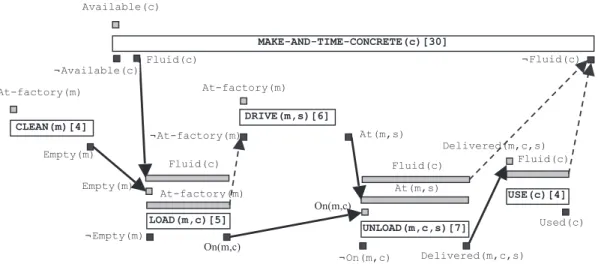
We represent non-instantaneous actions by a rectangle. The duration of an action is given in square brackets after the name of the action. Conditions are written above an action, and effects below. The action LOAD(m,c) shown in Figure 1 represents loading a batch of concrete c in a mixer m. We have Cond(LOAD(m,c)) = {Fluid(c), Empty(m), At-factory(m)}. We can see from the figure that the mixer must be empty at the start of the loading, whereas the concrete must be fluid and the mixer at the fac-tory during the whole duration of the loading. We have Del(LOAD(m,c)) = {Empty(m)} and Add(LOAD(m,c) = {On(m,c)}. We can see from the figure that as soon as loading starts, the mixer is no longer empty and at the end of loading the mixer contains the concrete.
Figure 1: An example of the representation of a durative action
We use the notation a → f to denote the event that action a establishes fluent f, a → ¬f to denote the event that a destroys f, and f |→ a and f →| a, respectively, to denote the beginning and end of the interval over which a requires the condition f. If f is already true (respectively, false) when the event
a → f (a → ¬f) occurs, we still consider that a establishes (destroys) f. A temporal plan may contain several instances of the same action, but since most of the temporal plans studied in this paper contain at most one instance of each action, for notational simplicity, we only make the distinction between actions and action-instances if this is absolutely necessary. We use the notation τ(e) to represent the time in a plan at which an event e occurs.
Fluid(c) LOAD(m,c)[5] At-factory(m) On(m,c) ¬Empty(m) Empty(m)
COOPER, MARIS, & REGNIER
For a given action (or action-instance) a, let Events(a) represent the different events which consti-tute its definition, namely (a → f) for all f in Add(a), (a → ¬f) for all f in Del(a), ( f |→ a) and ( f →| a) for all f in Cond(a). The definition of an action a includes constraints Constr(a) on the rela-tive times of events in Events(a). For example, the internal structure of the fixed-length action LOAD(m,c) shown in Figure 1 is defined by constraints such as
τ(Fluid(c) →| LOAD(m,c)) − τ(Fluid(c) |→ LOAD(m,c)) = 5 τ(LOAD(m,c) → On(m,c)) − τ(Fluid(c) →| LOAD(m,c)) = 0
As in PDDL2.1, we consider that the length of time between events in Events(a) is not necessarily fixed and that Constr(a) is a set of interval constraints on pairs of events, such as τ(f →| a) − τ(f |→ a) ∈ [α, β] for some constants α,β. We use [αa(e1, e2), βa(e1, e2)] to denote the inter-val of possible inter-values for the relative distance between events e1, e2 in action a. A fixed length of time between events e1, e2 ∈ Events(a) can, of course, be modelled by setting αa(e1, e2) = βa(e1, e2). Similar-ly, the absence of any constraint can be modelled by the interval [−∞, +∞]. We now introduce two basic constraints that all temporal plans must satisfy.
inherent constraints on the set of action-instances A: for all a∈A, a satisfies Constr(a), i.e. for all
pairs of events e1, e2 ∈ Events(a), τ(e1) − τ(e2) ∈ [αa(e1, e2), βa(e1, e2)].
contradictory-effects constraints on the set of action-instances A: for all ai, aj ∈A, for all positive
fluents f ∈ Del(ai) ∩ Add(aj), τ(ai → ¬f) ≠ τ(aj → f).
The inherent constraints define the internal structure of each action-instance, whereas the contradicto-ry-effects constraints ensure that the truth-value of each fluent never becomes undefined during the execution of a temporal plan. For example, if a plan contains an instance a of the action LOAD(m,c) shown in Figure 1 and an instance b of another action CLEAN(m) with Empty(m) ∈ Add(CLEAN(m)), then the temporal plan must satisfy the contradictory-effects constraint
τ(a → ¬EMPTY(m)) ≠ τ(b → EMPTY(m)).
Definition 3.1. A temporal planning problem <I,A,G> consists of a set of actions A, an initial state I
and a goal G, where I and G are sets of fluents.
Notation: If A is a set of action-instances, then Events(A) is the union of the sets Events(a) (for all
action-instances a ∈ A).
Definition 3.2. P = <A,τ>, where A is a finite set of action-instances {a1,...,an} and τ is a real-valued
function on Events(A), is a temporal plan for the problem <I,A′,G> if
(1) A ⊆ A′, and
(2) P satisfies the inherent and contradictory-effect constraints on A;
and when P is executed (i.e. fluents are established or destroyed at the times given by τ) starting from the initial state I:
(3) for all ai ∈ A, each f ∈ Cond(ai) is true when it is required, and
(4) all goal fluents g ∈ G are true at the end of the execution of P. (5) P is robust under infinitesimal shifts in the starting times of actions.
Events are instantaneous, whereas actions are not only durative but may also be of variable length. Thus a temporal plan P does not schedule its action-instances directly but schedules all the events in its action-instances.
Condition (5) in Definition 3.2 means that we disallow plans which require perfect synchronisation between different actions. Fox, Long and Halsey (2004) show how this condition can be imposed within PDDL2.1. We require that in all plans fluents are established strictly before the beginning of the interval over which they are required. The only exception to this rule is when a fluent f is estab-lished and required by the same action a. We allow the possibility of perfect synchronization within an action, which means that we can have τ(a → f) = τ(f |→ a). Similarly, fluents can only be destroyed strictly after the end of the interval over which they are required. The only exception to this rule is
when a fluent f is required and destroyed by an action a, in which case we can have τ(f →| a) =
τ(a → ¬f). For example, the fluent Empty(m) is simultaneously required and destroyed by the action LOAD(m,c) shown in Figure 1.
Since a set of actions can be viewed as a set of action-instances in which each action occurs exactly once, we can apply constraints, such as the inherent and contradictory-effects constraints, to a set of actions rather then a set of action-instances. We now look in more detail at the type of constraints that we impose on the relative times of events within an action-instance.
Definition 3.3. An interval constraint C(x,y) on real-valued variables x,y is a binary constraint of the
form x−y ∈ [a,b] where a,b are real constants.
Definition 3.4. (Jeavons & Cooper, 1995) A binary constraint C(x,y) is min-closed if for all pairs of
values (x1,y1), (x2,y2) which satisfy C, (min(x1,x2),min(y1,y2)) also satisfies C. A binary constraint
C(x,y) is max-closed if for all pairs of values (x1,y1), (x2,y2) which satisfy C, (max(x1,x2),max(y1,y2)) also satisfies C.
Lemma 3.5. Let A = {a1,...,an} be a set of actions and A′ a set of action-instances in which each action
ai (i=1,...,n) occurs ti≥1 times. Let τ be a real-valued function on the set of events in A′. For each
e ∈ Events(ai), let e[j] (j=1,...,ti) represent the occurrence of event e within instance number j of ai.
For i ∈ {1,...,n}, define the real-valued functions τmin,τmax on the set of events in the set of actions A by τmin(e) = min{τ(e[j])| j=1,...,ti} and τmax(e) = max{τ(e[j])| j=1,...,ti}. If τ satisfies the inherent
con-straints on A′, then both τmin and τmax satisfy the inherent constraints on A.
Proof: All interval constraints are both min-closed and max-closed (Jeavons & Cooper, 1995). By
applying the definition of min-closedness (respectively, max-closedness) ti −1 times, for each action ai,
we can deduce that if τ satisfies an interval constraint on each of the ti instances of ai, then τmin (τmax) satisfies this constraint on the action ai. In other words, for all pairs of events e1,e2 in Events(ai), if
τ(e1[j]) − τ(e2[j]) ∈ [αa(e1,e2), βa(e1,e2)] for j=1,...,ti, then τmin(e1) − τmin(e2) ∈ [αa(e1,e2), βa(e1,e2)] and τmax(e1) − τmax(e2) ∈ [αa(e1,e2), βa(e1,e2)]. Hence if τ satisfies the inherent constraints on A′, then τmin and τmax satisfy the inherent constraints on A. □
Definition 3.6. A temporal planning problem <I,A,G> is positive if there are no negative fluents in the
In this paper, we will only consider positive temporal planning problems <I,A,G>. It is well known that any planning problem can be transformed into an equivalent positive problem in linear time by the introduction, for each positive fluent f, of a new fluent notf to replace occurrences of ¬f in condi-tions of accondi-tions (Ghallab, Nau & Traverso, 2004). It is important to note, however, that this transfor-mation may not conserve other properties of the instance. By the assumption that all problems are pos-itive, G and Cond(a) (for any action a) are composed of positive fluents. By convention, Add(a) and Del(a) are also composed exclusively of positive fluents. The initial state I, however, may contain negative fluents.
For simplicity of presentation, we assume throughout this paper that the set of actions A has under-gone the filtering operation consisting of eliminating those actions a from A which cannot possibly be executed since Cond(a) is not a subset of I ∪ Add(A).
We will need the following notion of establisher-uniqueness in order to define our tractable class of temporal planning problems. This is equivalent to post-uniqueness in SAS+ planning (Jonsson & Bäckström, 1998) restricted to Boolean variables but specialised so that it applies to a specific subset of the positive fluents. In the next section, we apply it to the subset of positive fluents which may be required for the realisation of the goal.
Definition 3.7. A set of actions A = {a1,...,an} is establisher-unique (EU) relative to a set of positive
fluents S if for all i ≠ j, Add(ai) ∩ Add(aj) ∩ S = ∅, i.e. no fluent of S can be established by two
dis-tinct actions of A.
If a set of actions is establisher-unique relative to the set of sub-goals of a problem, then we can de-termine in polynomial time the set of actions which are necessarily present in a temporal plan. There remains the problem of determining how many times each action must occur and then scheduling the-se action-instances in order to produce a valid temporal plan. Establisher-uniqueness alone cannot prevent minimal plans from being of exponential size (Bäckström & Klein, 1991b).
4. Monotone Planning
In this section, we introduce the notion of monotonicity of fluents. Together with establisher-uniqueness, the monotonicity of fluents is a sufficient condition for the existence of a polynomial-time algorithm for temporal planning.
Definition 4.1. A fluent f is –monotone (relative to a positive temporal planning problem <I,A,G>) if,
after being destroyed f is never re-established in any temporal plan for <I,A,G>. A fluent f is
+monotone (relative to <I,A,G>) if, after having been established f is never destroyed in any temporal
plan for <I,A,G>. A fluent is monotone (relative to <I,A,G>) if it is either + or −monotone (relative to <I,A,G>).
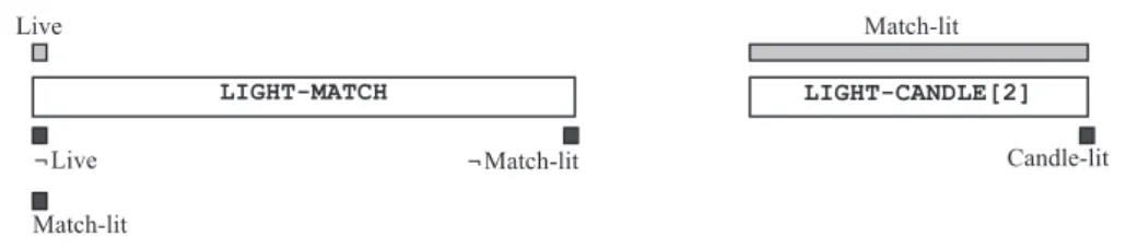
Example 4.2: Consider the two actions shown in Figure 2: LIGHT-MATCH and LIGHT-CANDLE.
The action LIGHT-MATCH requires that the match be live, in order to light it. The match remains lit until it is blown out at the end of the action. A constraint in Constr(LIGHT-MATCH) imposes that the duration of the action, i.e. τ(LIGHT-MATCH → ¬Match-lit) − τ(LIGHT-MATCH → Match-lit), is between 1 and 10 time units. The second action LIGHT-CANDLE requires that the match be lit
dur-ing two time units for the candle to be lit. For an initial state I = {live, ¬Match-lit} and a set of goals
G = {Candle-lit}, it is clear that all temporal plans for this problem involve executing the two actions
in parallel with the start (respectively, end) of LIGHT-MATCH being strictly before (after) the start (end) of LIGHT-CANDLE. There is only one match available, which means that LIGHT-MATCH can be executed at most once. This means that the fluent Match-lit is −monotone since it cannot be established after being destroyed. This same fluent Match-lit is not +monotone since it is destroyed after being established.
Figure 2: An example of a set of actions which allows us to light a candle using a single match.
Notation: If A is a set of actions, we use the notation Del(A) to represent the union of the sets Del(a)
(for all actions a ∈ A). Add(A), Cond(A), Constr(A) are defined similarly. The following lemma follows trivially from Definition 4.1.
Lemma 4.3. If f ∉ Add(A) ∩ Del(A), then f is both −monotone and +monotone relative to the positive
temporal planning problem <I,A,G>.
Certain physical actions or chemical reactions are irreversible. Examples include bursting a bal-loon, killing a fly, adding milk to a cup of coffee or burning fuel. Since there can be no action to de-stroy the corresponding fluents Burst, Fly-dead, Milk-added, Fuel-burnt, these fluents are necessarily both −monotone and +monotone by Lemma 4.3. A similar remark holds for fluents that may be true in the initial state but for which there is no action which establishes them, such as Fly-alive, for example. In Example 4.2, the fluent Live is both −monotone and +monotone since there is no action to estab-lish it, and the fluent Candle-lit is −monotone and +monotone since there is no action to destroy it.
We now introduce three other sets of constraints, the −authorisation constraints being applied to –monotone fluents f and the +authorisation constraints to +monotone fluents. The causality constraints on fluent f are only valid if there is a unique action-instance which establishes f.
−authorisation constraints on the positive fluent f and the set of action-instances A: for all ai ≠aj ∈A, if f ∈ Del(aj) ∩ Cond(ai), then τ(f →| ai) < τ(aj → ¬f); for all ai ∈ A, if f ∈ Del(ai) ∩
Cond(ai), then τ(f →| ai) ≤ τ(ai → ¬f).
+authorisation constraints on the positive fluent f and the set of action-instances A: for all ai,aj ∈ A,
if f ∈ Del(aj) ∩ Add(ai) ∩ (Cond(A) ∪ G), then τ(aj → ¬f) < τ(ai → f).
causality constraints on the positive fluent f and the set of action-instances A: for all ai≠aj ∈ A, if
f∈(Cond(aj) ∩ Add(ai))\I, then τ(ai → f) < τ(f |→ aj); for all ai ∈ A, if f ∈ (Cond(ai) ∩ Add(ai))\I then
τ(ai → f) ≤ τ(f |→ ai). LIGHT-MATCH LIGHT-CANDLE[2] ¬Live ¬Match-lit Match-lit Candle-lit Match-lit Live
Within the same action-instance ai, perfect synchronisation is possible between the events f →| ai
and ai → ¬f. Indeed, one way of ensuring that an action a is executed at most once in any temporal
plan is to create a fluent fa ∈ Cond(a) ∩ Del(a) ∩ I which is simultaneously required and deleted at
the start of a and which is established by no action. For example, when a is the action LIGHT-MATCH in Example 4.2, fa is the fluent live. On the other hand, by condition (5) of Definition 3.2 of a
temporal plan, we cannot have perfect synchronisation between events in distinct action-instances. This explains why the −authorisation constraints impose the strict inequality τ(f →| ai) < τ(aj → ¬f)
when ai ≠ aj but only the non-strict inequality τ(f →| ai) ≤ τ(aj → ¬f) when ai =aj. A similar remark
holds for the perfect synchronisation of the events ai → f and f |→ aj which is only permitted by the
causality constraints when ai =aj.
Definition 4.4. A temporal plan <A,τ> for a positive temporal planning problem <I,A′,G> is monotone
if each pair of action-instances (in A) satisfies the +authorisation constraints for all +monotone fluents and satisfies the –authorisation constraints for all –monotone fluents.
Definition 4.5. Given a temporal planning problem <I,A,G>, the set of goals is the minimum
sub-set SG of Cond(A) ∪ G satisfying 1. G ⊆ SG
2. for all a ∈ A, if Add(a) ∩ (SG\I) ≠ ∅, then Cond(a) ⊆ SG.
The reduced set of actions is Ar = {a ∈ A | Add(a) ∩ (SG\I) ≠ ∅}.
We can determine SG and then Ar in polynomial time and the result is unique. To see this consider the simple algorithm which initialises SG to G and then repeatedly adds to SG the set of fluents F which is the union of (Cond(a)\SG) over all actions a ∈ A such that Add(a) ∩ (SG\I) ≠ ∅, until F=∅. This simple algorithm has worst-case time complexity O(n3), where n is the total number of events in the actions of A, and produces a unique result which is clearly the minimum set of fluents satisfying the two conditions of Definition 4.5. Note that this algorithm is similar to the standard method of relevance detection used in GRAPHPLAN (Blum & Furst, 1995).
In order to state our theorem, we require a more relaxed definition of the set of sub-goals and the reduced set of actions to take into account the case in which fluents in the initial state are destroyed and re-established. Let SGp (the set of possible sub-goals) denote the minimal set of fluents satisfying
1. G ⊆ SGp
2. for all actions a ∈ A, if Add(a) ∩ SGp ≠ ∅ then Cond(a) ⊆ SGp.
Let Ap be the set of actions { a ∈ A | Add(a) ∩ SGp ≠ ∅ }. The difference between Ar and Ap is that
Ap is the set of actions which could occur in a minimal temporal plan in which fluents in the initial state can be destroyed and re-established. As with SG and Ar, SGp and Ap are unique and can be de-termined in O(n3) time.
If each fluent in Cond(Ar) ∪ G is monotone, we say that a plan P for the temporal planning prob-lem <I,A,G> satisfies the authorisation constraints if each −monotone fluent satisfies the −authorisa-tion constraints and each +monotone fluent satisfies the +authorisa−authorisa-tion constraints (it is assumed that we know, for each fluent f ∈ Cond(Ar) ∪ G, whether f is + or –monotone).
The following theorem contains minor improvements and corrections compared to the conference version of the present paper (Cooper, Maris & Régnier, 2012). Since it is a corollary of Theorem 5.6 (proved in the following section), we omit its proof.
Theorem 4.6. Given a positive temporal planning problem <I,A,G>, let SG and Ar be, respectively, the set of sub-goals and the reduced set of actions, with Ap defined as above. Suppose that Constr(Ar) are interval constraints, the set of actions Ar is establisher-unique relative to SG\ I, each fluent in Cond(Ar) ∪ G is monotone relative to <I,Ar,G> and each fluent in I ∩ (Cond(Ar) ∪ G) is –monotone relative to <I,Ap,G>. Then <I,A,G> has a temporal plan P if and only if
(1) G ⊆ (I\Del(Ar)) ∪ Add(Ar) (2) Cond(Ar) ⊆ I ∪ Add(Ar)
(3) all fluents g ∈ G ∩ Del(Ar) ∩ Add(Ar) are +monotone relative to <I,Ar,G>
(4) the set of authorisation, inherent, contradictory-effects and causality constraints has a solution over the set of actions Ar.
5. Extending Monotonicity of Fluents
In this section we introduce the notion of monotonicity*, thus allowing us to define a larger tracta-ble class of temporal planning protracta-blems.
Definition 5.1. A plan is minimal if removing any non-empty subset of action-instances produces an
invalid plan. A fluent f is –monotone* (relative to a positive temporal planning problem <I,A,G>) if, after being destroyed f is never re-established in any minimal temporal plan for <I,A,G>. A fluent f is
+monotone* (relative to <I,A,G>) if, after having been established f is never destroyed in any minimal
temporal plan for <I,A,G>. A fluent is monotone* (relative to <I,A,G>) if it is either + or −monotone* (relative to <I,A,G>).
Example 5.2. To give an example of a monotone* fluent which is not monotone, consider the
follow-ing plannfollow-ing problem in which all actions are instantaneous: Start_vehicle: k → o
Drive: o → d, ¬o Unload: d → p
with I = {k}, G = {p}. The fluents represent that I have they ignition key (k), the engine is on (o), the destination has been reached (d) and that the package has been delivered (p). There is only one mini-mal plan, namely Start_vehicle, Drive, Unload, but there is also the non-minimini-mal plan Start_vehicle, Drive, Start_vehicle, Unload in which the fluent o is established, destroyed and then re-established. Hence o is −monotone* but not −monotone.
A +monotone (−monotone) fluent is clearly +monotone* (−monotone*) since in any plan, includ-ing minimal plans, after havinclud-ing been established (destroyed) it is never destroyed (re-established). In order to prove the equivalent of Theorem 4.6 for monotone* fluents, we first require another definition and two minor technical results.
Definition 5.3. A minimal temporal plan <A,τ> for a positive temporal planning problem <I,A′,G> is
monotone* if each pair of action-instances in A satisfies the +authorisation constraints for all
+monotone* fluents and satisfies the –authorisation constraints for all –monotone* fluents.
The following lemma follows directly from Definition 5.1 of the monotonicity* of a fluent along with the fact that a fluent cannot be simultaneously established and destroyed in a temporal plan.
Lemma 5.4. Suppose that the positive fluent f is monotone* relative to a positive temporal planning
problem <I,A′,G>. Let <A,τ> be a minimal temporal plan for <I,A′,G> with actions ai,aj ∈ A such that
f ∈ Add(ai) ∩ Del(aj). If f is +monotone* relative to this problem, then τ(aj → ¬f) < τ(ai → f). If f is
–monotone* relative to this problem, then τ(ai → f) < τ(aj → ¬f).
Proposition 5.5. If each fluent in Cond(A) is monotone* relative to a positive temporal planning
prob-lem <I,A,G>, then all minimal temporal plans for <I,A,G> are monotone*.
Proof: Let P be a minimal temporal plan. Consider firstly a positive –monotone* fluent f. We have to
show that the −authorisation constraints are satisfied for f in P, i.e. that f is not destroyed before (or at the same time as) it is required in P. But this must be the case since P is a plan and f cannot be re-established once it is destroyed. Consider secondly a positive +monotone* fluent f. By Lemma 5.4, the +authorisation constraint is satisfied for f in P. □
We can now give our main theorem which generalizes Theorem 4.6 to monotone* fluents.
Theorem 5.6. Given a positive temporal planning problem <I,A,G>, let SG and Ar be, respectively, the set of sub-goals and the reduced set of actions. Suppose that all constraints in Constr(Ar) are inter-val constraints, the set of actions Ar is establisher-unique relative to SG\ I, each fluent in Cond(Ar) ∪ G is monotone* relative to <I,Ar,G> and each fluent in I ∩ (Cond(Ar) ∪ G) is –monotone* relative to <I,Ap,G>. Then <I,A,G> has a temporal plan P if and only if
(1) G ⊆ (I\ Del(Ar)) ∪ Add(Ar) (2) Cond(Ar) ⊆ I ∪ Add(Ar)
(3) all fluents g ∈ G ∩ Del(Ar) ∩ Add(Ar) are +monotone* relative to <I,Ar,G>
(4) the set of authorisation, inherent, contradictory-effects and causality constraints (given in Sec-tions 3 and 4) has a solution τ over the set of acSec-tions Ar (where the +authorisation constraints apply to each +monotone* fluent and the −authorisation constraints apply to each −monotone* fluent).
Proof: (⇒) If <I,A,G> has a temporal plan, then it clearly has a minimal plan P. Ar is the set of those actions which establish sub-goals f ∈ SG\ I. By definition, SG = Cond(Ar) ∪ G. Since Ar is establisher-unique relative to SG\ I, each sub-goal f ∈ SG\ I has a unique action which establishes it. Hence each action in Ar must occur in the plan P. Furthermore, (Add(A)\ Add(Ar)) ∩ (Cond(Ar)\I) = ∅ by
Defini-tion 4.5. It follows that (2) is a necessary condiDefini-tion for a temporal plan P to exist.
Let Pp be a version of P in which we only keep actions in Ap. Pp is a valid temporal plan since, by definition of Ap, no fluent in (Cond(Ap) ∪ G) can be established by actions in A\ Ap. Indeed, since P was assumed to be minimal, we must have Pp =P. Now let P′ be a version of P in which we only keep actions in Ar. By Definition 4.5, no conditions of actions in P′ and no goals in G are established by any
of the actions eliminated from P, except possibly if they are also in I. Thus to show that P′ is also a valid temporal plan we only need to show that any establishment of a fluent f ∈ I ∩ (Cond(Ar) ∪ G) in
P by an action a ∈ Ap \ Ar is unnecessary. By hypothesis, f is −monotone* relative to <I,Ap,G> and
hence f cannot be established in P after having been destroyed. Since f ∈ I, this means that the estab-lishment of f in P was unnecessary. Hence P′ is a valid temporal plan. Indeed, since P was assumed to be minimal, we must have P′=P.
We have seen that P contains exactly the actions in Ar. Hence, all fluents g∈G (which are neces-sarily positive by our hypothesis of a positive planning problem) that are either not present in the ini-tial state I or are deleted by an action in Ar must be established by an action in Ar. It follows that (1) is a necessary condition for P to be a valid temporal plan. Consider g ∈ G ∩ Del(Ar) ∩ Add(Ar). From Lemma 5.4, we can deduce that g cannot be −monotone*, since g is true at the end of the execution of
P. Thus (3) holds. Let Pmin=<Ar,τmin> be the version of the temporal plan P=<Ar,τ> in which we only keep one instance of each action ai ∈ Ar (and no instances of the actions in A\Ar) and τmin is defined from τ by taking the first instance of each event in Events(ai), for each action ai ∈ A
r
, as described in the statement of Lemma 3.5. We will show that Pmin satisfies the authorisation, inherent, contradicto-ry-effects and causality constraints.
We know that P is a temporal plan for the problem <I,A,G>. Hence it is also a temporal plan for the problem <I,Ar,G>, since it uses only actions from Ar. By hypothesis, all fluents in Cond(Ar) are monotone relative to <I,Ar,G>. Therefore, by Proposition 5.5, the temporal plan P is monotone*. Since
P is monotone* and by the definition of a temporal plan, the authorisation constraints are all satisfied. P must also, by definition of a temporal plan, satisfy the inherent and contradictory-effects constraints.
It follows from Lemma 3.5 that Pmin also satisfies the inherent constraints. Since the events in Pmin are simply a subset of the events in P, Pmin necessarily satisfies both the authorisation constraints and the contradictory-effects constraints.
Consider a positive fluent f ∈ (Cond(aj) ∩ Add(ai))\ I, where ai, aj ∈ A
r
. Since aj ∈ A
r
, we know that Add(aj) ∩ (SG\ I) ≠ ∅ and hence that Cond(aj) ⊆ SG, by the definition of the set of sub-goals SG.
Since f ∈ Cond(aj) we can deduce that f ∈ SG. In fact, f ∈ SG\I since we assume that f ∉ I. It follows
that if f ∈ Add(a) for some a ∈ A, then a ∈ Ar. But we know that Ar is establisher-unique (relative to
SG). Hence, since f ∈ Cond(aj) ⊆ Cond(Ar) and f ∈ Add(ai), f can be established by the single action
a=ai in A. Since f ∉ I, the first establishment of f by an instance of ai must occur in P before f is first
required by any instance of aj. It follows that the causality constraint must be satisfied by f in Pmin.
(⇐) Suppose that conditions (1)-(4) are satisfied by Ar. Let P be a solution to the set of authorisation, inherent, contradictory-effects and causality constraints over Ar. A solution to these constraints uses each action in Ar (in fact, it uses each action exactly once since it assigns one start time to each action in Ar). Consider any g ∈ G. By (1), g ∈ (I\Del(Ar)) ∪ Add(Ar). If g ∉ Del(Ar), then g is necessarily true at the end of the execution of P. On the other hand, if g ∈ Del(aj) for some action aj ∈ Ar, then by
(1) there is necessarily some action ai ∈ A
r
which establishes g. Then, by (3) g is +monotone*. Since P satisfies the +authorisation constraint for g, ai establishes g after all deletions of g. It follows that g is
true at the end of the execution of P.
Consider some –monotone* f ∈ Cond(aj) where aj ∈ A
r
. Since the –authorisation constraint is satisfied for f in P, f can only be deleted in P after it is required by aj. Therefore, it only remains to
show that f was either true in the initial state I or it was established some time before it is required by
aj. By (2), f ∈ I ∪ Add(A
r
), so we only need to consider the case in which f ∉ I but f ∈ Add(ai) for
some action ai ∈ Ar. Since P satisfies the causality constraint, τ(ai → f) < τ(f |→ aj) and hence, during
the execution of P, f is true when it is required by action aj.
Consider some f ∈ Cond(aj), where aj ∈ A
r
, such that f is not –monotone*. By the assump-tions of the theorem, f is necessarily +monotone* and f ∉ I. First, consider the case f ∉ Del(Ar) ∩ Add(Ar). By Lemma 4.3, f is −monotone (and hence −monotone*) which contradicts our assumption. Therefore f ∈ Del(ak) ∩ Add(ai), for some ai, ak ∈ Ar, and recall that f ∉ I. Since the +authorisation
constraint is satisfied for f in P, any destruction of f occurs before f is established by ai. It then follows
from the causality constraint that the condition f will be true when required by aj during the execution
of P. □
The makespan of a temporal plan P = <A,τ> is the time interval between the first and last events of
P, i.e. max{τ(e) | e∈Events(A)} − min{τ(e) | e∈Events(A)}. The problem of finding a plan with
min-imum makespan is polytime approximable if there is a polynomial-time algorithm which, given a temporal planning problem <I,A,G> and any ε>0, finds a temporal plan whose makespan is no more than Mopt +ε, where Mopt is the minimum makespan of all temporal plans for <I,A,G>.
If the constraints in Constr(a) impose that the time interval between each pair of events in Events(a) is fixed, then we say that action a is rigid.
We express complexities in terms of the total number n of events in the actions in A. Without loss of generality, we assume that all actions in A contain at least one event and all fluents occur in at least one event. Hence the number of actions and fluents are both bounded above by n.
Theorem 5.7: Let ΠEUM* be the class of positive temporal planning problems <I,A,G> in which A is establisher-unique relative to Cond(A) ∪ G, all fluents in Cond(A) ∪ G are monotone* relative to <I,A,G> and all fluents in I ∩ (Cond(A) ∪ G) are −monotone* relative to <I,A,G>. Then ΠEUM* can be solved in time O(n3) and space O(n2), where n is the total number of events in the actions in A. Indeed, we can even find a temporal plan with the minimum number of action-instances or of minimal cost, if each action has an associated non-negative cost, in the same complexity. Furthermore, if all actions in
A are rigid then the problem of finding a plan with minimum makespan is polytime approximable.
Proof: The fact that ΠEUM* can be solved in time O(n3) and space O(n2) follows almost directly from Theorem 5.6 and the fact that the set of authorisation, inherent, contradictory-effects and causality constraints form an STP≠, a simple temporal problem with difference constraints (Koubarakis, 1992). An instance of STP≠ can be solved in O(n3+k) time and O(n2+k) space (Gerevini & Cristani, 1997), where n is the number of variables and k the number of difference constraints (i.e. constraints of the form xj – xi ≠ d). Here, the only difference constraints are the contradictory-effects constraints of
which there are at most n2, so k=O(n2). Furthermore, as pointed out in Section 4, the calculation of SG and Ar is O(n3).
Establisher-uniqueness tells us exactly which actions must belong to minimal temporal plans. Then, as we have seen in the proof of Theorem 5.6, the monotonicity* assumptions imply that we only need one instance of each of these actions. It then trivially follows that we solve the optimal version of the temporal planning problem, in which the aim is to find a temporal plan with the minimum number of
action-instances or of minimal cost, if each action has an associated cost, by solving the set of authori-sation, inherent, contradictory-effects and causality constraints.
Now suppose that all actions in A are rigid. We will express the problem of minimising makespan while ignoring the contradictory-effects constraints as a linear program. We will then show that it is always possible to satisfy the contradictory-effects constraints (without violating the other constraints) by making arbitrarily small perturbations to the start times of actions. We assume that the events in a single action-instance satisfy the contradictory-effects and authorisation constraints; since actions are rigid this can be checked independently for each action in A in polynomial time. Let P be a temporal plan for <I,A,G> which has minimum makespan. We showed in the proof of Theorem 5.6 that Pmin, obtained from P by keeping only one instance of each action in P, is also a valid temporal plan. Since makespan cannot be increased by eliminating action-instances from a temporal plan, Pmin also mini-mises makespan. Let C be the set of inherent, authorisation and causality constraints that Pmin must satisfy. C contains equality constraints of the form xj – xi = d, where d is a constant and xj, xi are times
of events in the same action, and constraints of the form xj – xi < d, where d is a constant and xj, xi are
times of events in different actions. We introduce two other variables τbegin, τend and we denote by Copt the set of constraints C together with the constraints τbegin ≤ τ(e) and τ(e) ≤ τend for all e∈Events(A
r ). The linear program which minimises τend – τbegin subject to the constraints Copt minimises makespan but does not take into account the contradictory-effects constraints C≠ that must be satisfied by a valid
temporal plan. Let PLP be a solution to this linear program. Its makespan is clearly no greater than
Mopt, the minimum makespan of all temporal plans (since valid temporal plans must satisfy the con-straints C ∪ C≠). Let δ be the minimum difference d – (x
j – xi) in PLP over all constraints of the form
xj – xi < d in C. Let ∆ be the minimum non-zero difference |d – (xj – xi)| in PLP over all contradictory-effects constraints xj – xi ≠ d in C≠. Suppose that Ar = {a
1,...,am}. Let P be identical to PLP except that we add µi = min{ε,δ,∆}(i–1)/m to τ(e) for all e∈Events(ai). By construction, all contradictory-effects
constraints which were violated in PLP are satisfied in P, all contradictory-effects constraints which were satisfied in PLP are still satisfied in P, and all strict inequalities which were satisfied in PLP are still satisfied in P. The inequalities τbegin ≤ τ(e) are still satisfied in P. Finally, in order to guarantee satisfying the inequalities τ(e) ≤ τend, it suffices to add ε to τend. The resulting solution P corresponds to a valid temporal plan whose makespan is no more than Mopt +ε. The result then follows from the fact that linear programming is solvable in O(n3.5L) time by Karmarkar’s interior-point algorithm, where n
is the number of variables and L the number of bits required to encode the problem (Karmarkar,
1984). □
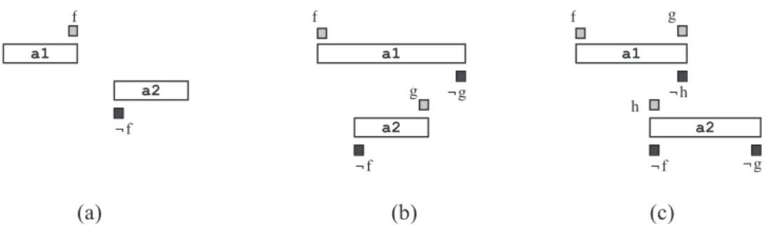
Figure 3: (a) all instances of action a1 occur strictly before all instances of action a2, (b) all instances of
a2 are contained in all instances of a1 (c) all instances of a1 overlap all instances of a2. a1 ¬f f a2 a1 ¬f f a2 ¬g g a1 ¬f f a2 ¬g g ¬h h (a) (b) (c)
In the class ΠEUM*, all sub-goal fluents f ∈ SG are true over a single interval Int(f, P) during the exe-cution of a temporal plan P. If f is +monotone*, then Int(f, P) is necessarily of the form [t1,∞) where t1 is the moment when f is first established. If f is −monotone*, then Int(f, P) is necessarily of the form [t1,t2] where t1 is again the moment when f is first established (or 0 if f ∈ I) and t2 is the first moment after t1 when f is destroyed (or [t1,∞) if f is never destroyed). The class ΠEUM* is solvable in polynomial time due to the fact that establisher-uniqueness ensures that there is no choice concerning which ac-tions to include in the plan and monotonicity* ensures that the only choice concerning the time of events is within an interval. Given these two restrictions it is quite surprising that a large range of in-dustrial planning problems fall in this class (Cooper, Maris & Régnier, 2012, 2013b). EU monotone planning is a sufficiently powerful modelling language to allow us to impose constraints such as an action occurs at most once in a plan or that all instances of event e1 occur before all instances of event
e2. To illustrate this, Figure 3 shows how we can impose precedence, containment or overlapping con-straints between actions a1 and a2 by the introduction of, respectively, one, two or three fluents
f,g, h ∈ I which occur only in the events shown in Figure 3. By Lemma 4.3, these fluents f,g,h are all
necessarily both −monotone and +monotone in all temporal plans.
6. Temporal Relaxation
Relaxation is ubiquitous in Artificial Intelligence. A valid relaxation of an instance I has a solution if I has a solution. Hence when the relaxation has no solution, this implies the unsolvability of the original instance I. A tractable relaxation can be built and solved in polynomial time.
The traditional relaxation of propositional non-temporal planning problems consisting of ignoring deletes has two drawbacks. Firstly, it is traditionally used with a forward search, which is not valid in temporal planning unless some specific transformation has been applied beforehand to the set of ac-tions (Cooper, Maris & Régnier, 2013a). Secondly, it does not use information which may be essential for the detection of unsolvability of the original instance, namely the destruction of fluents and tem-poral information such as the relative duration of actions. In this section we present a valid tractable relaxation inspired by EU monotone temporal planning. In the following section we show how to use our temporal relaxation to detect monotonicity* of fluents. There are other possible applications, such as the detection of action landmarks (actions which occur in each solution plan) (Karpas & Domshlak, 2009), which immediately leads to a lower bound on the cost of a plan when each action has an asso-ciated cost (Cooper, de Roquemaurel & Régnier, 2011).
The traditional relaxation of classical non-temporal planning problems consists of ignoring deletes of actions. By finding the cost of an optimal relaxed plan, this relaxation can be used to calculate the admissible h+ heuristic. As shown by Betz and Helmert (2009), h+ is very informative but unfortu-nately NP-hard to compute (Bylander, 1994) and also hard to approximate (Betz & Helmert, 2009). As this relaxation does not use information which may be essential for the detection of un-solvability of the original instance (namely the destruction of fluents), a lot of research has been carried out to take some deletes into account (Fox & Long, 2001; Gerevini, Saetti & Serina, 2003; Helmert, 2004; Helmert & Geffner, 2008; Keyder & Geffner, 2008; Cai, Hoffmann & Helmert, 2009). Another recent approach (Haslum, Slaney & Thiébaux, 2012; Keyder, Hoffmann & Haslum, 2012) consists in enrich-ing the classical relaxation with a set of fact conjunctions. Finally the red-black relaxation (Katz, Hoffmann & Domshlak, 2013a, 2013b) generalizes delete-relaxed planning by relaxing only a subset of the state variables.
Unfortunately, these relaxations do not directly generalize to temporal planning, since techniques based on a combination of ignoring deletes and forward search are not valid in temporal planning un-less some specific transformation has been applied beforehand to the set of actions. An important as-pect of temporal planning, which is absent from non-temporal planning, is that certain temporal plan-ning problems, known as temporally-expressive problems, require concurrency of actions in order to be solved (Cushing, Kambhampati, Mausam & Weld, 2007). A typical example of a temporally-expressive problem is cooking: several ingredients must be cooked simultaneously in order to be ready at the same moment. In a previous paper (Cooper, Maris & Régnier, 2010), we identified a sub-class of temporally expressive problems, known as temporally-cyclic, which require cyclically-dependent sets of actions in order to be solved.
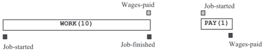
Figure 4: An example of a temporally cyclic temporal planning problem.
A simple temporally-cyclic problem is shown in Figure 4, where I = ∅ and G = {Job-finished}. A condition for a workman to start work is that he is paid (at the end of the job) whereas his employer will only pay him after he has started work. In a valid temporal plan for this problem the actions PAY and WORK must be executed in parallel with the execution of action PAY contained within the inter-val over which action WORK is executed. After applying the traditional ignore-deletes relaxation, forward chaining from the initial state would not be able to start either of the two actions since both of them have a missing condition. Thus, certain proposed techniques, although very useful in guiding heuristic search (Eyerich, Mattmüller & Röger, 2009; Do & Kambhampati, 2003), are not valid for temporally cyclic problems. Different solutions exist to get round the problem of temporal cycles. For example, we gave a polynomial-time algorithm to transform a temporally-cyclic problem into an equivalent acyclic one (Cooper, Maris & Régnier, 2013a). Other transformations have been proposed in the literature (Long & Fox, 2003; Coles, Fox, Long & Smith, 2008) which also eliminate the possi-bility of temporal cycles, although this was not an explicitly-stated aim in the descriptions of these transformations: temporal cycles are avoided by decomposing durative actions into instantaneous ac-tions denoting the start and end of the action. Intermediate condiac-tions can also be managed by splitting actions into component actions enclosed within an “envelope” action (Smith, 2003). In each case, ig-noring deletes in the transformed problem followed by forward search provides a valid relaxation. If the original problem is not temporarily cyclic, then ignoring deletes followed by forward search is a valid relaxation.
In this section, we present an alternative form of relaxation, which we call TR (for Temporal Re-laxation), inspired by EU monotone planning, comprising an STP≠ instance which has a solution only if the original temporal planning instance has a solution. It is incomparable with the relaxation based on ignoring deletes, as we will show through temporal and non-temporal examples, in the sense that there are instances that can be detected as unsolvable using EU monotone relaxation but not by ignor-ing deletes (and vice versa).
WORK(10)
Job-started Job-finished Wages-paid Job-started Wages-paid
By applying the following simple rule until convergence we can transform (in polynomial time) any temporal planning problem P into a relaxed version P′ which is EU relative to the set of sub-goals
SG: if a sub-goal fluent f is established by two distinct actions, then delete f from the goal G and from
Cond(a) for all actions a. As a consequence, f is no longer a sub-goal and SG has to be recalculated. Clearly, P′ is a valid relaxation of P. From now on we assume the temporal planning problem is EU relative to SG.
We denote by ALM the set of action landmarks that have been detected (Karpas & Domshlak, 2009). Action landmarks are also known as indispensable actions (Cooper, de Roquemaurel & Ré-gnier, 2011). Establisher-uniqueness implies that we can easily identify many such actions, in particu-lar the set of actions Ar which establish sub-goals not present in the initial state I.
We cannot assume in the STP≠ that a single instance of each action will be sufficient. For each ac-tion landmark aand for each event e ∈ Events(a), we introduce two variables τfirst(e), τlast(e) represent-ing the times of the first and last occurrences of event e in the plan. The constraints of our temporal relaxation TR include versions of the internal, contradictory-effects, authorization and causality con-straints (which we give below) together with the following obvious constraint:
intrinsic TR-constraints: ∀a∈ALM, for all events e ∈ Events(a), τfirst(e) ≤ τlast(e).
In the conference version of this paper in which we described a preliminary version of TR (Cooper, Maris & Régnier 2013b), we made the assumption that no two instances of the same action can over-lap. Under this assumption, for e1,e2 ∈ Events(a), the first occurrences of e1,e2 in a plan correspond to the same instance of action a. A similar remark holds for the last occurrences of e1,e2. It turns out that we do not need to make this assumption in order to apply in TR each inherent constraint in Constr(a) independently to the values of τfirst(e) and τlast(e) (for each e ∈ Events(a)). Indeed, according to Lem-ma 3.5, assuming that Constr(Ar) are interval constraints, if each instance of action a satisfies its inher-ent constraints, then both τfirst and τlast satisfy the inherent constraints on events in action a:
inherent TR-constraints: ∀a∈ALM, ∀ e1,e2 ∈ Events(a), τfirst(e1) − τfirst(e2) ∈ [αa(e1,e2), βa(e1,e2)] and τlast(e1) − τlast(e2) ∈ [αa(e1,e2), βa(e1,e2)].
The contradictory-effects constraints in TR are as follows:
contradictory-effects TR-constraints: ∀ai,aj ∈ ALM, for all positive fluents f ∈ Del(ai) ∩ Add(aj),
∀L1,L2 ∈ {first,last}, τL1(ai → ¬f) ≠ τL2(aj → f).
For each positive fluent f which is known to be −monotone*, we apply in TR the following modi-fied version of the −authorisation constraints on f:
−authorisation TR-constraints: ∀ ai ≠aj ∈ ALM, if f ∈ Del(aj) ∩ Cond(ai), then τlast(f →| ai) <
τfirst(aj → ¬f); for all ai ∈ A
LM
, if f ∈ Del(ai) ∩ Cond(ai), then τlast(f →| ai) ≤ τfirst(ai → ¬f).
For each positive fluent f which is known to be +monotone*, we apply in TR the following modified version of the +authorisation constraints on f:
+authorisation TR-constraints: ∀ai,aj ∈ ALM, if f ∈ Del(aj) ∩ Add(ai), then τlast(aj → ¬f) <
τfirst(ai → f).
We check that every condition and every goal can be established, i.e. Cond(ALM) ⊆ I ∪ Add(A) and